This is a repository copy of
Controlled comparison of machine vision algorithms for Rumex
and Urtica detection in grassland
.
White Rose Research Online URL for this paper:
http://eprints.whiterose.ac.uk/117717/
Version: Accepted Version
Article:
Binch, A and Fox, CW orcid.org/0000-0002-6695-8081 (2017) Controlled comparison of
machine vision algorithms for Rumex and Urtica detection in grassland. Computers and
Electronics in Agriculture, 140. pp. 123-138. ISSN 0168-1699
https://doi.org/10.1016/j.compag.2017.05.018
© 2017, Elsevier. Licensed under the Creative Commons
Attribution-NonCommercial-NoDerivatives 4.0 International
http://creativecommons.org/licenses/by-nc-nd/4.0/
[email protected] https://eprints.whiterose.ac.uk/
Reuse
Items deposited in White Rose Research Online are protected by copyright, with all rights reserved unless indicated otherwise. They may be downloaded and/or printed for private study, or other acts as permitted by national copyright laws. The publisher or other rights holders may allow further reproduction and re-use of the full text version. This is indicated by the licence information on the White Rose Research Online record for the item.
Takedown
If you consider content in White Rose Research Online to be in breach of UK law, please notify us by
Controlled comparison of machine vision algorithms
1for Rumex and Urtica detection in grassland
2A Binch a,c, CW Fox b,c
a School of Computing, b Institute for Transport Studies,
The University of Leeds, LS2 9JT, United Kingdom.
c Ibex Automation Ltd, S35 7DQ, United Kingdom.
Corresponding author: [email protected] Submitted to Computers and Electronics in Agriculture 3
May 16, 2017 4
Abstract
5Automated robotic weeding of grassland will improve the productivity of dairy and sheep farms 6
while helping to conserve their environments. Previous studies have reported results of machine 7
vision methods to separate grass from grassland weeds but each use their own datasets and 8
report only performance of their own algorithm, making it impossible to compare them. A 9
definitive, large-scale independent study is presented of all major known grassland weed detec-10
tion methods evaluated on a new standardised data set under a wider range of environment 11
conditions. This allows for a fair, unbiased, independent and statistically significant comparison 12
of these and future methods for the first time. We test features including linear binary pat-13
terns, BRISK, Fourier and Watershed; and classifiers including support vector machines, linear 14
discriminants, nearest neighbour, and meta-classifier combinations. The most accurate method 15
is found to use linear binary patterns together with a support vector machine.1 16
1
1
Introduction
17Automated robotic weeding of grassland will improve the productivity of dairy and sheep farms 18
while helping to conserve their environments. At present grassland weeding is typically per-19
formed in two styles. Tractor-mounted bulk spraying of selective herbicides is expensive due to 20
the volume, and cost per unit of selective chemicals. Manual backpack-mounted spraying uses 21
lower, targeted spot spray doses of generic herbicides such as glyphosate, but requires more 22
expensive manual labour time. Precision robots [4, 6] present an opportunity to use similarly 23
low and targeted doses of cheap generic herbicides as in the manual case, but at much lower 24
cost as they can drive, detect and spray automatically without the need to pay manual sprayers 25
by the hour. Precision robots could further eliminate the need for chemical herbicide altogether 26
by destroying detected weeds with mechanical or other non-chemical methods. Data collected 27
about weed locations by robots can be fed into geospatial weed mapping systems to enable 28
ecological analyses. 29
Autonomous weeding robots must first detect weeds at a suitable resolution and accuracy. 30
Machine vision provides many tools and algorithms for detection, with varying performances, 31
and can be cheap to operate using consumer-grade cameras. Several previous studies have 32
reported results of machine vision methods to separate grass from grassland weeds, typically 33
Rumex obtusifolius(dockleaf). But as is common in early stages of artificial intelligence research, 34
they each use their own datasets and report only performance of their own algorithm rather than 35
presenting controlled trials testing methods against one another. As proof of concept studies, 36
many used only small data sets, did not report confidence intervals on their accuracy rates, 37
and have not yet tested methods across lighting and weather conditions which are known to 38
affect many vision algorithms. It is well known in artificial intelligence that unintended author 39
bias and bottom drawer effects can creep into studies when the same author both designs and 40
tests an algorithm, so there is a need for independent validation. We present a large-scale (tens 41
of thousands of images), independent study of all major grassland weed detection methods 42
evaluated on a new standardised data set, under a wider range of environment conditions. This 43
allows for a fair, unbiased, independent and statistically significant comparison of the methods 44
1.1 Previous work
46
Previous studies can be grouped roughly into those which classify individual windows (patches) 47
of images (e.g. tens of pixels square) independently of one another, and those which apply mor-48
phological operations to whole images (e.g. hundreds or thousands of pixels width and height). 49
Window-based methods compute features of the windows such as spectra or texture descriptors, 50
while whole-image methods try to isolate shapes via segmentation algorithms. Window-based 51
methods include: [10] used local binary pattern (LBP) texture features with a per pixel threshold 52
Rumex/Grass classifier, under controlled artificial lighting conditions, to report between 87%-53
97% accuracy on a test set of 941 images of 50x40 pixels. [2] uses very large windows to obtain 54
high accuracy, 98.5%, using texture features and support vector machine (SVM) classification. 55
Whole-image segmentation methods include: [12] segmented images into regions of similar tex-56
ture then classified the shapes of these regions, reporting 71%-95% accuracy in Rumex/(Grass 57
and mixed herbs) classification under constant lighting conditions. [27] used thresholded and 58
segmented Fast Fourier Transforms (FFT) to detect Rumex in grass on 161 images, reporting 59
94% accuracy. [33] used a similar setup to report accuracies 82%-89% for Rumex/Grass. [31] 60
used segmentation (erosion and dilation). [17] use Gray Level Co-occurrence Matrix and Laws’ 61
filter mask texture features with linear discriminant analysis (LDA) and segmentation to report 62
90% Rumex/Grass. [18] use Markov Random Field based texture features and segmentation to 63
report a 97.8% accuracy on 92 images. A summary of the key properties of each method is 64
66
study method classes reported number of illumination window
accuracy test images size
[10] LBP+threshold R/G 87%-97% 941 artificial 50×40
[12] Segment+shape R/(G+H) 71%-95% 3681 windows constant n/a
[27] FFT+segment R/G 94% 161 images constant 8
[33] FFT+segment R/G 82%-89% 56 images constant 8
[31] Segment R/G 89% 240 images constant n/a
[17] GLCM+LDA+segment R 90% 92 images constant n/a
[18] MRF segment R/G 97.8% 92 images constant n/a
[2] LBP+SVM R 98.5% 400 images varied 320×240
67
From the table, it is clear that making a fair comparison of these algorithms is difficult 68
or impossible from publicly available data. Each study uses its own data sets, comprising 69
completely different images and conditions. In many cases the separation of training and test 70
data is not clear, with studies reporting best results having optimised parameters over the 71
same test set used in the final result, rather than making a clean train/test separation. It is 72
well-known [11] that optimising parameters to the test set tends to yield over-optimistic results 73
compared to performance on new data. Some studies do not describe the variation in the 74
lighting conditions, but are assumed to be constant conditions because they use small numbers 75
of test images collected, presumably, on the same day. Window-based methods have used 76
different window sizes, while whole-image segmentation methods make use of data from across 77
the whole image to classify each local pixel, which is hard to meaningfully evaluate against 78
windowed results. Window size is important because it represents a fundamental trade-off 79
between detection accuracy and spatial resolution. A large window contains more information 80
which will yield high accuracies, but at the cost of a lower spatial resolution, for example in 81
determining what area of ground to spray with herbicide. 82
In our native UK grassland, Rumex is not the only common weed and almost always co-83
occurs with similar populations of Urtica diotica (stinging nettle). As such, any automated 84
grassland weeding system needs to work with both Rumex and Urtica together. If Rumex 85
only was precision sprayed, then a selective bulk spray for Urtica would still be needed which 86
chemicals are available. Previous work on automatic detection of Urtica in grassland has relied 88
on non-visual spectral methods including near infra-red and full hyper-spectra [23, 24, 38], but 89
these sensors are more costly than simple visual cameras. Urtica has smaller leaves than Rumex 90
which makes it harder to detect with machine vision alone, in particular some Rumex detection 91
methods rely entirely on obvious features of the large, smooth Rumex leaves, which may not 92
carry over to the Urtica case. However Urtica has distinctive jagged edges on its leaves which 93
suggest that methods based on such local shapes (rather than texture) features may be useful 94
for detection. 95
With the exception of [2], all the systems in table 1 rely on vertical camera angles, i.e. 96
cameras mounted to look directly downwards at the ground. This simplifies recognition as there 97
is no perspective, and all parts of the ground look the same. However this imposes physical 98
limitations on precision robots, which must either mount a camera physically outside the robot’s 99
base footprint, or inside the body of the robot looking directly under its base. Much UK 100
grassland is found in less-favoured areas, including hilly and rocky terrain such as sheep farms. 101
These terrains often include obstacles which robots must navigate around, and such navigation 102
is complicated by physical extrusions beyond robot platform bases such as cameras on arms or 103
beams. Similarly, robots designed for these terrains may need heavy, protective bases which 104
prevent cameras or sprayers from being mounted directly downwards from them. To generalise 105
operation beyond flat grassland to cases such as these, it is more convenient and lower-cost to 106
use more standard camera mountings on top of the robot body, with cameras facing forwards 107
and tilted down, as in [2]. While this is a more robust physical solution, it makes the machine 108
vision problem harder as it must now deal with perspective. Further, the previous studies all 109
use clean images taken by stationary cameras to ease recognition. In practice, precision robots 110
operating in generalised terrains will be moving at speed, capturing images during motion. It is 111
not practical to stop every time an image must be taken. While camera stabilisation systems are 112
available at a cost, grassland and especially hill farmers typically require lower budget solutions 113
than arable farmers, so it is of interest to test algorithms on data collected from similar moving 114
robot platforms as would be used in practice, which can include motion blur. 115
Recent work has begun to explore the use of 3D lidar based sensing and detection of Rumex 116
interest, it is beyond the scope of the present machine vision study. Also beyond our scope 118
are non-visual approaches to weed detection including hyper-spectral [23, 24, 38], and chemical 119
sensing methods [26]. Our scope of detection of weeds in grassland is a particular sub-field of 120
automated weed detection in general, which has developed a wider range of methods applicable 121
to simpler cases of crops and weeds growing in flat, row-crop settings, which can typically 122
simplify the task by initial segmentation into green and brown discrete plant and soil regions, 123
unlike the grassland case where everything is green [7, 14, 21, 32, 36, 36]. 124
1.2 Data and algorithm requirements
125
To make a fair and useful comparison between the different algorithm types proposed for UK, 126
less-favoured area grassland weed recognition, and to extend the robustness of previous studies, 127
the following requirements were taken into account. 1. Data should be clearly split into training 128
and test sets. 2. Only a single run should be allowed of each algorithm on the test set. 3. The 129
algorithms should be implemented and tested independently of their original proposers. 4. 130
testing should be on Urtica as well as Rumex. 5. Data should be collected from a moving, 131
robust platform, with cameras mounted on top of its body and pitched downwards from the 132
plane. 6. Data size should be in the order order of thousands of image windows. 7. Classification 133
should be performed on standard sized windows, including for morphological methods which 134
should be restricted to run on the same windows as feature-based methods. 8. Windows should 135
be of a suitable spatial size and resolution to enable precision spraying. 9. Data should be 136
collected over a representative variety of different days, illumination, and weather conditions. 137
Taken together, these requirements are more challenging than settings used in the previous 138
studies. An independent evaluation should not seek to ‘sell’ any one algorithm with high rates, 139
and should not shy away from reporting low accuracies when they occur. This helps to avoid 140
any publication bias [28] which may have acted as a filter on previous tests. Due to interactions 141
between the requirements and differences in data types, we do not re-implement algorithms 142
directly but instead use similar or closely related methods. This is required in particular for 143
the morphological approaches which do not transfer directly to window classification, such as 144
the use of watershed segmentation to represent region based methods previously run on whole 145
as a whole rather than directly re-implementing and competing between them. 147
2
Methods
148
The objective of the experiments is to report, to a statistically significant level, the classification 149
performance of various classification methods for grass vs weed detection, i.e two-way classifi-150
cations representing spray/no-spray decisions for a general herbicide. In general this is distinct 151
from the problem of recognising individual weed species. A ‘classification method’ or ‘method’ 152
means a combination of one feature type with one classifier type. Care must be taken to avoid 153
contamination of classifier training with any information from test data. 154
2.1 Image acquisition and pre-processing
155
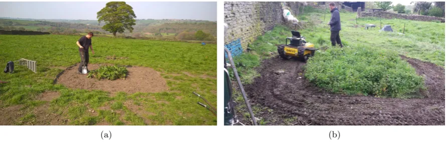
Test plots of weeds in grass were constructed on a dairy grassland farm in South Yorkshire, UK. 156
Slabs of Urtica approximately 0.2m squared were extracted from working fields and transplanted 157
into a 3m squared trench (Figure 2a). This process was repeated for Rumex. Transplanting real 158
slabs from areas of the working farm ensures maximum realism and avoids problems of growing 159
the weeds artificially, which could lead to unrealistic soil backgrounds in images. In particular, 160
the transplanted slabs also contain grass, soil, rocks, and other surface features of the real work-161
ing grassland farm, though only in 0.2m squared slabs which human transplanters considered to 162
be fully ‘sprayable’. To make this decision, the human transplanters were instructed to collect 163
only slabs which they would be happy to completely spray with a manual backpack sprayer if 164
they were being employed to manually destroy weeds. The weedy turfs were watered daily for 165
two weeks to allow the plants to stabilise before data collection. Plots were located in a region 166
of the farm that is in direct sunlight (not in shade) throughout the day. 167
Stereo pair images2 were acquired in 1080HD from each plot using auto-focusing cameras3 168
2
Only the mono, left camera images are used in this study. Stereo images were captured for use in future comparison studies and are also made available as part of the dataset.
3
(C920, www.logitech.com) mounted on a tracked robot as in fig. 1. The cameras were fixed 169
to the robot’s left side, facing out at right angle yaw to the direction of travel, and at π/8 170
radians (22.5 degrees) pitch down, to give a view over a roughly 1m square area of ground. The 171
robot drove in circles around the plots whilst capturing pictures, randomised between 0m and 172
1m from the edge of the plots (figure 2b). This guarantees an equal balance of lighting and 173
shadow angles in the data, because each drive around the plot contains images of the plot from 174
all ground angles. The size of the plots, robot, and camera positions were selected such that 175
the plot contents fill the images. This setup removes the need for manual annotation of weed 176
classes in images, as we are assured that every part of every image is full of a weed class. One 177
image was taken every second. 178
Image acquisition was arranged into epochs, where a single epoch consisted of making re-179
peated revolutions of each plot for a period of ten minutes (yielding twenty minutes of weed 180
image acquisition from the two weed types together), followed by fifteen minutes of grass image 181
acquisition. The open grassland contained a mixture of grasses including Lolium multiflorum, 182
Festuca pratensis, Phleum pratense, and Holcus lanatus with some Trifolium repens (clover). 183
Approximately half of the epochs were acquired under overcast weather conditions, whilst the 184
other half was acquired under bright or sunny weather conditions. Data capture was staged 185
over four days, with 10 epochs in total captured at random times of day from sunrise to sunset 186
during May 2016. Images were inspected manually and a small portion (<0.1%) removed due 187
to recording problems. Approximately a third of a terabyte of usable image data was thus 188
acquired in total, to our knowledge this is the largest and most multi-conditioned data set of 189
its kind. 190
Images were pre-processed in three steps: colour calibration, perspective dewarping, and 191
windowing. 192
In colour calibration, images are transformed to compensate for variations due to lighting 193
and weather conditions. Colour calibration acts to colour-standardise images (to a certain 194
extent) to simplify classification. It was performed using a colour bar present in all images, 195
recorded as part the robot camera frames (Figure 3). The colour bar was composed of five 196
coloured squares (red, blue, yellow, white and green) using standard colours of paint. A single 197
Figure 1: Camera geometry. Showing position of camera on tracked robot (viewed from the front), facing sideways. The thick black square shows the area on the ground, in perspective, used later in the perspective transform.
(a) (b)
Figure 2: Image acquisition. a) Weed plot construction. b) Images were obtained using cameras mounted to the side of a tracked robot. The robot repeatedly made revolutions of each plot whilst taking pictures.
reference image was selected to calibrate all other images to. A measure of the blue, red and 198
green light intensities from each coloured square on the bar was obtained as the mean value of 199
the red, green and blue channels within the square. For each channel a vector of intensities was 200
constructed with values for each coloured square, yielding the vectorsbr,gr andrr for the blue,
201
red and green channels, respectively. The subscript r indicates that these values are from the 202
reference image. Repeating this procedure for a comparison image c (i.e. an image that is to 203
be colour calibrated) gives vectors bc,gc and rc. A linear relationship between the intensities
204
of the blue, red and green channels is assumed, measured from the reference image and the 205
intensities of the blue, red and green channels measured from the comparison image. Given this 206
assumption, the parameters for each channel, for example blue, are obtained as βˆ(b), 207
ˆ
β(b) = (X(b)TX(b))−1X(b)Tb
[image:10.595.80.526.267.409.2](a) (b) (c)
[image:11.595.70.554.83.302.2](d) (e) (f)
Figure 3: Colour Calibration. Figures a, b and c are raw images of dock leaves before any pre-processing has taken place. Figures d, e and f are colour calibrated versions of figures a, b and c, respectively.
where 208
X(b) =
redr(b) 1
bluer(b) 1
..
. ...
greenr(b) 1
,bc =
redc(b)
bluec(b)
.. .
greenc(b)
, (2)
where the values in the left hand column of the matrixX(b) is the vectorbr. These parameters
209
are used to colour calibrate the blue channel of the comparison image as: 210
I′ c(b) =
Ic(b)−βˆ(b)[1]
ˆ
β(b)[2] , (3)
where the term in square brackets indexes a value in βˆ(b), I is the original intensity andI′
is 211
the adjusted intensity. Performing these operations for the green and red channels also yields a 212
fully colour calibrated image. 213
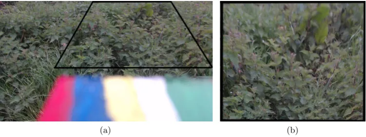
Perspective normalisation was performed via the projective transform shown in fig. 4a to 214
those in fig. 4b. This maps a 1.16m width by 1.0m depth ground area into a 700 pixel width 215
by 600 pixel height image, whose geometry is identical to that of a vertical, overhead camera 216
(a) (b)
Figure 4: Perspective normalisation. a) Raw image from left camera, with grid annotation showing 1.16m width x 1m depth on the ground. b) Affine transformation to remove perspective, grid annotation showing locations of the same rectangle after perspective transformation into a 600x700 pixel image.
camera due to the three dimensional structure of the plants. In particular, tall plants at the 218
front of the image are inflated in size because they are warped as if they were further back. 219
A key research question asks whether this will have a detrimental effect over pure overhead 220
imaging. 221
Finally the dewarped image was split into regular 28×28 square or 64×64 square pixel win-222
dows for classification, corresponding to 46mm or 106mm squares of ground space respectively. 223
Windows were contiguous and non-overlapping, and were stored for analysis. (These sizes were 224
chosen to be around the scale of a single spray target radius, or ground size of a single weed or 225
clump of weeds. 64 is a power of two which speeds up FFT based methods; 28 rather than 32 is 226
chosen for the smaller window size to enable future comparisons with neural network methods, 227
where 282 pixel windows are a common standard for historical and technical reasons [16].) 228
2.2 Dataset definitions
229
To avoid test data contaminating training processes, the set of epochs was first partitioned into 230
training epochs and test epochs. This prevents, for example, classifiers from learning to recognise 231
the lighting conditions rather than the weed types. Partitioning was performed manually to 232
ensure a balance of weather conditions and weed types in each partition. 233
After partitioning the epochs, we defined training and hyper-training datasets by sampling 234
windows from the test epochs. (Separate hyper-training and hyper-test sets are used during 236
hyper-parameter optimisation before training proper, to avoid contamination by test set data, 237
as described in section 2.5.) A data set consisted of a set of images, where half of those were 238
images of grass and the other half were images of weeds. A data set could contain an individual 239
weed type (Rumex or Urtica) or a mixture of weed types (Rumex and Urtica). Similarly, a data 240
set could contain images obtained under individual weather conditions (overcast or sunny) or a 241
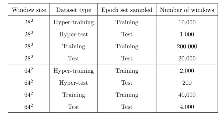
mixture of weather conditions (overcast and sunny). The data set sizes are shown in the table 242
[image:13.595.117.469.278.461.2]below, 243
Table 1: Dataset sizes. 244
Window size Dataset type Epoch set sampled Number of windows
282 Hyper-training Training 10,000
282 Hyper-test Test 1,000
282 Training Training 200,000
282 Test Test 20,000
642 Hyper-training Training 2,000
642 Hyper-test Test 200
642 Training Training 40,000
642 Test Test 4,000
245
These sizes are still small compared with the total amount of raw data collected, but are 246
orders of magnitude larger than data used in previous studies. 247
4 The test set size was chosen to yield significant confidence in the results, while the training
248
set size was selected to enable all the software implementations to train within one day of 249
processing on a single 3GHz Intel core. Test and hyper-test datasets are 10% size of their 250
corresponding training and hyper-training sets. The 282 sets are set to contain 5 times as many 251
images as the 642 sets so that they contain the same amount of total pixel data (282 ≈642/5), 252
4
to allow results to be meaningfully compared across window sizes. 253
2.3 Feature extraction
254
The windowed images contain 642 or 282pixels of RGB data, which are too large to use directly 255
as input vectors to most classifiers. Therefore, features were first computed from the data, as 256
in the previous studies. The selection of features used is detailed below and was selected to 257
represent most previously proposed feature choices. All features ran on greyscale versions of 258
the windows (obtained as the mean of the RGB channels), which is justified as all images are 259
primarily all the same shade of green (unlike the case in detection studies of arable crop weeds 260
in brown soil). 261
2.3.1 Fourier Transform 262
The Fourier Transform [39] represents an image in the basis of its orthogonal harmonic frequency 263
components. For digital images the discrete Fourier transform (DFT) is used, whose basis is a 264
set of two dimensional harmonics large enough to fully describe the spatial domain image. The 265
number of frequencies corresponds to the number of pixels in the spatial domain image. For a 266
square image of sizeN ×N, the two-dimensional DFT is given by: 267
F(k, l) =
N−1 X
i=0 N−1
X
j=0
f(i, j)e−ι2π(ki N
lj
N), (4)
wheref(i, j) is the image in the spatial domain and the exponential term is the basis function 268
corresponding to each pointF(k, l) in the Fourier space. The basis functions are two dimensional 269
sinusoidal waves of increasing spatial frequencies, i.e. F(0,0) represents the DC-component of 270
the image which corresponds to the average brightness and F(N −1, N −1) represents the 271
highest frequency. The absolute values of the DFT yield the image’s magnitude of frequency 272
spectrum which is used as the feature vector for classification. We denote this method of feature 273
extraction as FT. The Fourier transform is illustrated in figure 5, which shows that broad leaves 274
tend to contain stronger low spatial frequencies while grass’ thin blades give rise to higher spatial 275
2.3.2 Local binary patterns 277
Local binary patterns (LBP) are a texture description feature [15]. Local means they are 278
computed on local sub-windows of an image only, as a function of a center pixel and either its 279
immediate or r pixel radius neighbours; binary means that the feature vector is binary, with 280
each feature classed as either present or absent. Windows are converted to greyscale, then for 281
each pixelxi,j in the window, LBP computes an 8-element binary vector,
282
[(xi,j > xi,j+r),(xi,j > xi−r,j+r),(xi,j > xi−r,j),(xi,j > xi−r,j−r),(xi,j > xi,j−r),(xi,j >
283
xi+r,j−r),(xi+r,j > xi,j),(xi,j > xi+r,j+r)].
284
There are 28 = 256 possible values of this feature vector, with oriented edge and corner
285
detection present as special cases. LBP computes feature vector for each pixel in the window, 286
then computes a 256-point histogram of the obtained values over the window. The shapes of 287
these histograms are considered to be characteristic of the texture classes and are given as input 288
to classifiers. As well as using the eight near neighbours as above, a hyper-parameter npoints
289
can also be used to generalise to other numbers of quantised comparison points equally spaced 290
on a circle around the center. (Many other variations on the LBP concept have also been 291
proposed [13] but are beyond the scope of the present comparison study.) 292
2.3.3 Interest points and k-means 293
The above features treat every pixel in the window as equally important, and are considered to 294
represent texture-like properties. An alternative approach is to locate only ‘interesting’ points 295
within the window and base classification on these. In particular, weeds such as Urtica have 296
many distinctive jagged corners which might form useful points on which to base classification. 297
Interest point method contain two feature extraction steps prior to classification. First, interest 298
points are located; second, the local region at each of these points is used to extract a feature 299
descriptor. Points are considered interesting if they contain a mixture of colours and can be 300
uniquely located, i.e. a corner is interesting because there is only one location where it exists, 301
while an edge is less interesting because it exists along a line of locations. Feature classes used to 302
describe these points are usually wavelet-like, combining color, frequency and size information. 303
erties has been and remains an active area of machine vision research [25], but the present study 305
arbitrarily selects the state-of-the-art Scale-Invariant Center-Surround Detectors (CenSurE) [1] 306
interest point detector and the Binary Robust Invariant Scalable Keypoints (BRISK) [20] de-307
scriptor to represent the general class of methods. CenSurE finds an approximation to the set 308
of corner-like points defined by, 309
{λd(H(x)i,j)> t, d∈ {1,2}}, (5)
whereλdare the two eigenvalues of the Hessian matrixH of the imagex at each pixeli, j, and
310
tis a threshold. Both eigenvalues are maximal at corners of any rotation. Rather than compute 311
this computationally intensive (due to eigenvalue finding) test for every pixel, CenSurE first 312
performs a faster pre-screening step, using a set of scaled filters to approximate the Laplacian 313
(total curvature) at each pixel, then only computing the Hessian test at local maxima of this 314
curvature [1]. 315
BRISK descriptors are similar to the LBP vectors above, but using pixel intensity compar-316
isons, 317
fn= (xi,j > xi′
n,jn′), (6)
at a larger set of 256 offsets {an, bn}giving (i′n=i+an, jn′ =j+bn). Unlike LBP, these offsets
318
are not equally spaced around a circle, but may form any arbitrary pattern. Together with the 319
larger number of points, this may capture potentially higher-order information than in LBP. 320
Standard values of the offset patterns are used as provided in [20]. 321
When BRISK feature vectors have been computed for all images in the training set they are 322
passed to the k-means algorithm which clusters them into K regions in feature space, where 323
feature space is a finite p-dimensional vector space with each dimension representing a BRISK 324
feature of an image. Initiating K random clusters we firstly calculate the Euclidean distance 325
between theith BRISK vector xi and thekth cluster Ck
326
di,k =
p X
j=1
(xij −Ckj)2
1/2
. (7)
cluster that minimises d (Equation 7). This operation is then performed for each BRISK 328
vector. Knowing the members of each group we can now compute the new centroid of each 329
group based on these new memberships. New centroids are the average coordinates among new 330
members, 331
Ck= PNk
n=1Xn1
Nk
, ...,
PNk
n=1Xnp
Nk
, (8)
whereNkis the number of BRISK vectors in clusterk. This whole process is then repeated until
332
the BRISK vectors cease to move groups (i.e. until the computation of the k-means clustering 333
has reached stability). 334
Clustering observed BRISK vectors in this way defines K discrete types of BRISK feature. 335
For any given image, we may now extract each of its interest points, compute a BRISK descriptor 336
at these points, then replace each of their BRISK descriptors with one of these quantised types. 337
This allows us to then count how many ck of each discrete BRISK types k = 1 : K appear in
338
the image. The vector of these counts, {ck}k=1:K is then used as a feature descriptor of the
339
whole image. 340
We refer to this feature asB > K, (for ‘BRISK followed byk-means’). 341
2.3.4 Watershed segmentation 342
We wish to test window-based features against region-growing type methods as proposed in 343
previous studies. To make a fair comparison it is necessary to substitute pure region growing 344
with a similar but window-based method. Otherwise the region growing methods could be 345
accused of accessing more data to make classifications of each region, from the whole image, 346
rather than just from its local window. For this purpose, we use a watershed method as a close 347
substitute. Watershed segmentation [37] was originally developed for the purpose of separating 348
touching objects in an image rather than for classification, but may also be used as a region-349
growing type classifier. The watershed transform finds ‘catchment basins’ and ‘watershed ridge 350
lines’ in an image by treating it as a surface where light pixels are high and dark pixels are low. 351
Segmentation using the watershed transform works better if a human operator can first identify, 352
or ‘mark’, pixels from foreground objects and background locations. The marker-controlled 353
(a) (b) (c)
(d) (e) (f)
[image:18.595.130.446.78.420.2](g) (h) (i)
Figure 5: Feature extraction. Figures a, d and g are fully pre-processed images containing grass, Urtica and Rumex leaves, respectively. Figures b, e and h are the local binary patterns (LBPs) of images a, d and g, respectively (with n = 24, r = 4). Figures c, f and i are the magnitude of frequency spectra of images a, d and g, respectively.
Given a grey-scale image as input, we apply Otsu’s thresholding [37] to segment the back-355
ground from the foreground. Then we compute the Euclidean distance transform which com-356
putes the Euclidean distance to the closest zero (i.e. background pixel) for each of the foreground 357
pixels. Doing this yields the distance mapd. Next we apply a functionf(d, dmin) that finds the
358
peaks (local maxima) in the distance map, and ensures that we have at least a dmin pixel
dis-359
tance between each peak. Then we apply a connected component analysis using 8-connectivity 360
to the output of f, the output of which gives us our markers, which we then feed in to the 361
watershed function. The watershed function returns a matrix of labels, an array with the same 362
width and height as the input image. Each pixel value has a unique label value. Pixels that 363
have the same label belong to the same object. For a given image, we then count the number 364
of unique labels or segments. Performing these operations for multiple values of dmin yields
multiple counts of segments for a given image, and thus a feature vector for classification. We 366
denote this method of feature extraction as W. 367
2.4 Classifiers
368
The following classifiers were used to represent previously proposed architectures. Each classifier 369
(SVM, LDA, NN) can take as its input any feature type obtained from windows (LBP, FT, BiK, 370
W). This yields 12 distinct classification methods, LBPiSVM, FTiSVM, BiKiSVM, WiSVM, 371
LBPiLDA, FTiLDA, BiKiLDA, WiLDA, LBPiNN, FTiNN, BiKiNN and WiNN. For example, 372
LBPiSVM means that we pass the local binary pattern feature vector as input to a support 373
vector machine, whilst FTiLDA means that we pass the image’s frequency spectrum magnitude 374
feature vector as input to linear discriminant analysis. 375
2.4.1 Support Vector Machines 376
A Support Vector Machine [35] models the a classification problem as finding a non-linear 377
partition of the feature vector space into classes (e.g. grass or weeds), formed as a linear 378
partition of a higher-dimension space formed by non-linear high-dimensional projection of the 379
feature vectors. To understand how SVMs work it is useful to first briefly describe the support 380
vector classifier (SVC). The SVC separates images into their classes by finding the linear affine 381
hyper-plane that maximises the distance (known as the margin M) between the two image 382
classes in feature space. Observations that fall on the boundaries of the margin are the support 383
vectors. 384
The linear affine hyper-plane is defined by the following inner product, 385
b·x+b0= 0, b0 6= 0, (9)
where x is a p−dimensional training image feature vector with associated weights b. Now 386
consider a set of n p−dimensional training image feature vectors, xi, each with an associated
387
class labelyi ∈ {−1,1}. Introducing new hyper-parameters;n ǫi values (known as slack values)
388
and a hyper-parameterC (known as the budget), then we wish to maximiseM acrossb1, ..., bp,
ǫ1, ..., ǫnsuch that
390
p X
j=1
b2j = 1, (10)
391
yi(b·x+b0)≥M(1−ǫi),∀i = 1, ..., n, (11)
392
ǫ≥0,
n X
i=1
ǫi ≤C, (12)
whereC, the budget, is a non-negative ‘tuning’ hyper-parameter and hyper-parametersǫi allow
393
the individual observations (i.e. training images) to be on the wrong side of the margin or 394
hyper-plane. C collectively controls how much the individualǫi can be modified to violate the
395
margin. 396
SVMs are an extension of SVCs that results from a non-linear enlargement of the feature 397
space through the use of functions known as kernels. This enlargement of the feature space 398
means that observations from different classes can be separated in many more ways than they 399
could be otherwise. To obtain the SVM, firstly we note that it is possible to show that a linear 400
support vector classifier for a particular observation can be represented as a linear combination 401
of inner products for the subset ℓof training observations that represent the support vectors, 402
f(x) =b0+ X
i∈ℓ
αihx,xii, (13)
where αi are the coefficients. Replacing the inner product hxi,xki with a more general inner
403
product ‘kernel’ function K = K(xi,xk), we can modify the SVC representation to use
non-404
linear kernel functions. One example is the radial (RBF) kernel, 405
K(xi,xk) = exp
−γ p X
j
(xij−xkj)2
, γ >0. (14)
Intuitively, the γ parameter defines how far the influence of a single training example reaches, 406
with low values meaning ‘far’ and high values meaning ‘close’. Theγ parameter can be seen as 407
the inverse of the radius of influence of samples selected by the model as support vectors. 408
The algorithmic solution for the SVM is one that finds optimal values for the coefficientsα
409
and the slack variablesǫi. Typically gradient decent algorithms are used. The hyper-parameters
410
Finally, a test image is classified according to whether its feature vector x∗
results in a 412
positive or negative sign when passed into the function f(x∗). Note that feature vectors were
413
normalised before being passed into the support vector machine. We denote this classifier as 414
SVM. 415
2.4.2 Linear Discriminant Analysis 416
As with SVCs/SVMs, Linear Discriminant Analysis [22] models the classification problem by 417
creating a feature space with a dimension for each feature. However, in LDA, observations from 418
2 separate classes are assumed to be sampled from 2 separate multivariate Gaussian distributions 419
in feature space with different means but the same covariance matrix. Given those assumptions 420
we have a linear hyperplane perfectly separating the means of the 2 distributions. This means 421
that any observation that is situated above the hyperplane has a higher probability of being a 422
sample from the Gaussian whose mean is situated above the hyperplane than being a sample 423
from the Gaussian whose mean is located below the hyperplane. 424
To explain LDA in some more detail, firstly we write Bayes’ rule for the classification prob-425
lem 426
P(i|x) = PP(x|i)P(i) jP(x|i)P(i)
, (15)
where the likelihood function P(x|i) gives the probability that the observation x is a sample 427
from the Gaussian representing the classiandP(i) is the prior probability of the classi. From 428
Bayes’ rule and the assumptions outlined we can derive the linear discriminant analysis formula 429
fi =miC−1xTk −
1 2miC
−1mT
i + log(pi), (16)
where mi is a vector containing the mean of each feature for the class i and C is the pooled
430
within group covariance matrix which is a weighted mean of the covariance matrix Ci for each
431
class. For a total ofn observations, N classes and ni observations in each class Cis
432
C= 1
n
N X
i=1
niCi. (17)
Then we simply assign a test imagekto groupithat has maximumfi. We denote this classifier
as LDA. 434
2.4.3 ‘Nearest Neighbour’ Classifier 435
Nearest neighbour is a very simple classifier, used here to provide a baseline to compare with 436
the two more sophisticated classifiers (SVM and LDA) above. In its training phase, the nearest 437
neighbour classifier computes the median feature vector for each class (grass or weeds). A test 438
image is then classed as grass if its feature vector minimises the sum of absolute errors between 439
it and the median feature vector computed from grass images. Likewise a test image is classed 440
as containing weeds if its feature vector minimises the sum of absolute errors between it and 441
the median feature vector computed from images containing weeds. We denote this classifier as 442
NN. 443
2.5 Hyper-parameter optimisation
444
Some of the classifiers and features have hyper-parameters which define how training is com-445
puted. Previous studies have mostly reported the best obtained results of methods on test sets, 446
and stated the hyper-parameter values used to give them. However it is unclear whether the 447
hyper-parameters in these cases have been set in advance of the evaluation on the test sets, or 448
if they have been fit to the test data by running method multiple times on the test data and 449
reporting only the best result. 450
To avoid this potential bias, careful use was made of hyper-training and hyper-test datasets, 451
independent of both training and test datasets, to select hyper-parameters in advance of the 452
main training and test phases. Hyper-parameters were optimised on these sets, so that each 453
system only saw the final test set only once for its reportable evaluation score. 454
In theory, hyper-training could be performed by training many versions of a classifier on the 455
full training dataset, then scoring them against a hyper-test set, and selecting the best performer. 456
(The hyper-test sets are sometimes known as ‘validation sets’). However this requires running 457
time-consuming training many times. So given the large ratio of data to compute resources 458
available for this study, a smaller hyper-training dataset, of 5% size of the full training dataset, 459
available compute resources. 462
SVMs have two hyper-parameters (C and γ) that should be optimised. We set C and γ
463
in exponentially growing sequences,C = 2−5,2−3, ...,215,γ = 2−15,2−13, ...,23, which has been
464
shown to be a practical method for identifying good parameters [19]. In addition the parameters 465
(number of pointsnpointsand radiusr) of the LBP should also be optimised. For all experiments
466
we set npoints = 2,4, ...,30. For experiments with 282 pixel windows we setr = 1,2, ...,8 while
467
for experiments with 642 pixel windows we setr = 2,4, ...,16 (r has maximum value equal to a 468
quarter of the image width). For all experiments involving the BiK method of feature extraction 469
we optimisedK for valuesK= 1, ...,28. For all experiments involving the W method of feature 470
extraction we optimised the minimum distance term dmin in growing sequences of integers
471
[1],[1,2], ...,[1, ...,15]. For the sequence [1,2], for example, we would generate a feature vector 472
by first setting dmin = 1, passing an image into the W method and retrieving the number of
473
segments. Then the process would be repeated fordmin = 2 and both segment values would be
474
appended, yielding a feature vector of length 2. Thus the length of a particular sequence is the 475
length of the feature vector generated by the W method of feature extraction. 476
In addition to numerical hyper-parameters, SVMs can further use various kernels and LDA 477
can further use various types of ‘solver’ and both SVMs and LDA have an option to apply a 478
‘shrinking’/‘shrinkage’ heuristic. For the LBPiSVM method we reduced the number of param-479
eter permutations to consider by assuming some independence between parameters. Thus we 480
first optimised C and γ, (considering all permutations of C, γ) for a fixed npoints = 15, r = 4
481
for 282 pixel windows and a fixedn
points= 15,r = 8 for 642 pixel windows, for each kernel with
482
the shrinking heuristic turned on and off. Then we fixed C, γ and the kernel at their optimal 483
values and optimised npoints and r (considering all permutations of npoints, r). For all other
484
classification methods we considered all possible parameter permutations. 485
LDA’srand BRISK’s CenSurE approximation variables were also treated as hyper-parameters. 486
Details of the results on the test set from training that are used to set hyper-487
2.6 Experiments
489
After hyper-parameter optimisation, we evaluated the performance of each feature-classifier 490
combination by training from scratch on the full training dataset and testing for the first and 491
only time on the test dataset. 492
To enable a fair comparison of systems running on the two different window sizes, more 493
windows were present in the 282 pixel training and test sets than in the 642 pixel sets. This is 494
because each 64 pixel image contains roughly five times as much visual information as each 28 495
pixel image (282/642 = 0.19); each 642 pixel image is effectively five 282 pixel windows joined
496
together. Therefore, in the 282 pixel case, we used a training set of 200,000 windows and a test
497
set of 20,000 windows, each comprised of half grass and half weed windows; while in the 642 498
pixel case we used 1/5 as many windows: 40,000 training and 4,000 test, also comprised of half 499
grass and half weeds. 500
The most important practical question for weeding robots is the performance in mixed weeds 501
(Rumex+Urtica) and in mixed weather (sunny+overcast), for the two window sizes. Window 502
size is important because it controls the spatial resolution at which the robot could spray the 503
weeds – in square windows of 106mm or 56mm. As the key research question, performance was 504
evaluated for every one of the twelve feature-classifier combinations on both window sizes. 505
It is sometimes the case in machine learning that improved accuracies can be obtained by 506
fusion results from multiple methods into meta-classifiers (also known as ensemble learning). 507
Many combination algorithms are available with different and subtle assumptions which are still 508
sometimes debated [8, 9].5 To give a simple illustrative, though non-optimal, idea of what per-509
formance improvements could be available, three simple, standard fusion methods were tested. 510
First, a simple voting scheme, META-VOTE, assigns an equal weight to each classifier’s output, 511
and yields the classification with the most votes. (In the case of a tie, the best classifier’s output 512
is given the deciding vote.) Second, META-ACC weights the votes of each classifier by its ac-513
curacy. Finally, META-LDA considers the output of each classifier as an element of a Boolean 514
5
feature, and trains a new LDA classifier to predict ground truth class from these vectors.6 515
Secondary questions of interest include the effects of perspective, weather type, weed type, 516
and windowing. As a full training process can take several days, these questions were examined 517
using only the best feature+classifier system and assumed to be independent of one another. 518
To examine the effect of perspective unwarping, the test set (containing grass under mixed 519
weather conditions, and mixed weeds under mixed weather conditions), was split into new test 520
sets according to their windows’ vertical locations (row numbers) in the camera images for indi-521
vidual scoring. Low row numbers indicate windows from the base of the image, corresponding 522
to space close to the robot cameras, while high row numbers indicate windows at the top of the 523
image, from space furthest from the robot cameras. 524
To examine the effect of weather, each epoch was classified as sunny or overcast, and the 525
original test set was split into two test sets comprised of windows of these weather types for 526
individual evaluation. 527
To examine the effect of weed type on classifier performance, two set sets were created which 528
contained only grass-and-Urtica and grass-and-Rumex respectively, for individual evaluation. 529
To give an idea of performance in the limiting case of large windows full of weeds or grass, 530
we assessed the performance of the BiKiSVM classification method on full sized (600×700) 531
pixel windows from data sets containing grass vs mixed and individual weed types under mixed 532
weather conditions. We conducted this experiment because BRISK features are more usually 533
extracted from full-view images than from the standardised windows used in the rest of this 534
study. Thus we wished to asses the performance of this particular classification method under 535
its own ideal conditions. As with other experiments, hyper-parameters were optimised on 536
hyper-training and hyper-test datasets (though of new 600×700 windows and set sizes hyper-537
training=1000, hyper-test=200, training=10,000,test=2000 , before training and testing on the 538
training and test datasets. 539
6
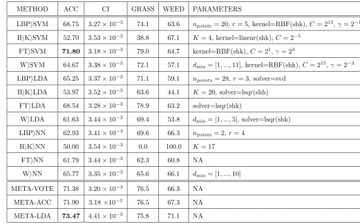
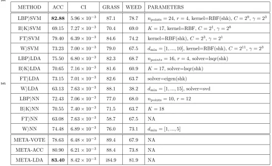
Table 2: Results of applying all 12 classification methods to 282 pixel window test dataset containing grass vs mixed weeds, mixed weather, after training on 282 pixel window training dataset. ACC is over all accuracy, i.e. the probability that a random image is correctly classified. CI is the confidence interval in the estimate of ACC. GRASS and W EED are probabilities that images of grass, or weed, respectively, are correctly classified. ‘NA’ stands for ‘Not Applicable’, ‘shk’ for ‘shrinking’.
540
541
METHOD ACC CI GRASS WEED PARAMETERS
LBPiSVM 68.75 3.27×10⁻³ 74.1 63.6 npoints= 20,r= 5, kernel=RBF(shk),C= 213,γ= 2−1
BiKiSVM 52.70 3.53×10⁻³ 38.8 67.1 K= 4, kernel=linear(shk), C= 2−5
FTiSVM 71.80 3.18×10⁻³ 79.0 64.7 kernel=RBF(shk),C= 21,γ= 23
WiSVM 64.67 3.38×10⁻³ 72.1 57.1 dmin= [1, ...,11], kernel=RBF(shk),C= 215,γ= 2−3
LBPiLDA 65.25 3.37×10⁻³ 71.1 59.1 npoints= 28,r= 3, solver=svd
BiKiLDA 53.97 3.52×10⁻³ 63.6 44.1 K= 20, solver=lsqr(shh)
FTiLDA 68.54 3.28×10⁻³ 78.9 63.2 solver=lsqr(shk)
WiLDA 61.63 3.44×10⁻³ 69.4 53.8 dmin= [1, ...,5], solver=lsqr(shk)
LBPiNN 62.93 3.41×10⁻³ 69.6 66.3 npoints= 2,r= 4
BiKiNN 50.00 3.54×10⁻³ 0.0 100.0 K= 17
FTiNN 61.79 3.44×10⁻³ 62.3 60.8 NA
WiNN 65.77 3.35×10⁻³ 65.6 66.1 dmin= [1, ...,10]
META-VOTE 71.38 3.20×10⁻³ 76.5 66.3 NA
META-ACC 71.90 3.18×10⁻³ 76.5 67.3 NA
META-LDA 73.47 4.41×10⁻³ 75.8 71.1 NA
Table 3: Results of applying all 12 classification methods to 642 pixel window test dataset containing grass vs mixed weeds, mixed weather, after training on 642 pixel window training dataset. ACCis over all accuracy, ie. the probability that a random image is correctly classified.
CIis the confidence interval in the estimate ofACC. GRASSandW EEDare probabilities that images of grass, or weed, respectively, are correctly classified. ‘NA’ stands for ‘Not Applicable’, ‘shk’ for ‘shrinking’.
543
544
METHOD ACC CI GRASS WEED PARAMETERS
LBPiSVM 82.88 5.96×10⁻³ 87.1 78.7 npoints= 24,r= 4, kernel=RBF(shk),C= 29,γ= 23
BiKiSVM 69.15 7.27×10⁻³ 70.4 69.0 K= 17, kernel=RBF,C= 21,γ= 28
FTiSVM 79.40 6.39×10⁻³ 84.6 74.2 kernel=RBF(shk),C= 23,γ= 21
WiSVM 73.23 7.00×10⁻³ 79.0 67.5 dmin= [1, ...,10], kernel=RBF(shk),C= 211,γ= 23
LBPiLDA 75.50 6.80×10⁻³ 82.3 68.7 npoints= 16,r= 4, solver=lsqr(shk)
BiKiLDA 70.65 7.16×10⁻³ 81.6 60.9 K= 17, solver=lsqr(shk)
FTiLDA 73.15 7.01×10⁻³ 82.6 63.7 solver=eigen(shk)
WiLDA 63.13 7.63×10⁻³ 88.1 38.2 dmin= [1, ...,15], solver=svd
LBPiNN 72.43 7.06×10⁻³ 77.0 68.0 npoints= 10,r= 12
BiKiNN 70.55 7.40×10⁻³ 71.5 63.7 K= 18
FTiNN 63.08 7.63×10⁻³ 58.7 67.5 NA
WiNN 74.48 6.89×10⁻³ 76.0 73.1 dmin= [1, ...,5]
META-VOTE 78.63 6.48×10⁻³ 89.4 67.9 NA
META-ACC 80.90 6.21×10⁻³ 88.4 73.8 NA
META-LDA 83.40 8.42×10⁻³ i84.9 81.9 NA
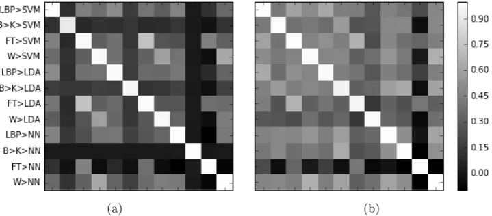
(a) (b)
Figure 6: Covariance Matrices. a) Covariance between the 12 classification methods when applied to 28 pixel squared windows (grass vs mixed weeds, mixed weather). b) Covariance between the 12 classification methods when applied to 64 pixel squared windows (grass vs mixed weeds, mixed weather).
3
Results
546
Tables 2 and 3 give the results for training and testing the 12 classification methods on 282 and
547
642 pixel windows, respectively, both with mixed weather and mixed weed types. ACC shows 548
the overall accuracy of each method, as the proportion of images correctly classified. Bayesian 549
confidence intervals (CI) computed as standard deviations of the Beta distribution posteriors 550
over belief in the accuracy [5], assuming flat priors, are also given for each classification method, 551
which justify the significance of the accuracy percentages to two decimal places. (We also list 552
breakdown accuracies for grass and weed image presentations, which indicate rates of false 553
positive and false negatives.) These experiments were conducted to determine which classifier 554
was the most accurate in predicting test images from data sets containing mixed weeds and 555
mixed weather conditions. 556
The LBPiSVM method performed better than the other classification methods for experiments 557
using 642 pixel windows, with an accuracy of 82.88%. This was achieved with the SVM kernel 558
set to RBF with the shrinking heuristic turned on, the hyper-parameters of the LBP set to 559
npoints= 24, r= 4 and the hyper-parameters of the SVM set toC= 29,γ = 23. The FTiSVM
560
method performed better than the other classification methods for experiments using 282 pixel 561
windows, with an accuracy of 71.80%. This was achieved with the SVM kernel set to RBF with 562
the shrinking heuristic turned on, and the SVM hyper-parameters set toC = 21,γ = 23.
282 and 642 pixel windowed cases. This may be due to averaging of the best method with the 565
less good methods dragging down the overall result. This typically occurs when all or most 566
classifiers are acting on the same inherent information in the data but with different accuracies, 567
rather than acting on different types of information per method. Similarly, META-ACC gives 568
on a tiny improvement over the best method for 282 windows (71.90 vs 71.80), and is worse
569
than the best 642pixel method (80.90 vs 82.88). META-LDA is the best of the meta-classifiers, 570
and is the only one to give significant improvements in both the 282 pixel (73.74 vs 71.80) 571
and 642 pixel (83.40 vs 82.88). (Significance can be seen by comparing the small CIs with the 572
larger accuracy differences). META-LDA’s weights are more principled, and optimal under its 573
assumptions, than the heuristic META-VOTE and META-ACC, so its better performance is 574
expected. However the gain from using META-LDA over using just the single best method, in 575
each window case, is small. Again, this suggested that all the methods are operating on similar 576
information within the images rather than with different information. Further insight into this 577
possibility is gained by examining the correlation matrix of the 12 methods’ predictions in fig. 578
6. Here, each grass/weed classification in the test set is considered to have a value of 0 or 1 for 579
grass/weed, and correlations over the test data are presented. It can be seen that the methods 580
are less correlated with one another in the 282 pixel case than in the 642 pixel case, which 581
explains why meta-classification works better for 282 than 642 windows. There are stronger 582
correlations between methods sharing the same feature type than methods sharing the same 583
classifier type, as can be seen by the secondary diagonal patterns. The FT>NN method has a 584
low correlation with the others because it is a very poor accuracy method. 585
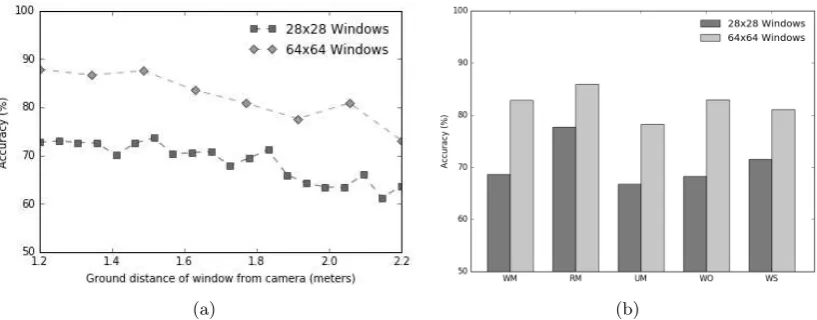
Results for the distance experiment are shown in Figure 7a. The best performing feature-586
classifier combination - the LBPiSVM method - is here run again on mixed weed and weather 587
test sets, separated as a function of the distance of the window from the robot camera’s ground 588
location (for both 282 and 642 pixel-squared windows). Classification performance decreased 589
smoothly as the distance increased, for both 282 and 642 pixel windows, by a considerable 590
amount (by around 15% absolute for 642 windows, and 10% absolute for 282 windows.) Weeds 591
closest to the cameras were predicted with a 87.85% accuracy (for 642 pixel windows), which
592
is more in line with the high accuracies reported by the previous studies than with accuracies 593
at far distances. It should also be noted that this result was obtained for a mixture of Rumex 594
(a) (b)
Figure 7: Effects of distance, weed type and weather. a) Classification performance of LBPiSVM as a function of the distance from the robot cameras (experiments on grass vs mixed weeds, mixed weather). b) Classification performance of LBPiSVM as a function of weed type (W: mixed weeds, R: Rumex, U: Urtica) and weather type (M: Mixed weather, O: Overcast, S: Sunny).
Results of the weed type and weather experiments are shown in 7b, again using the LBPiSVM 596
method. Here W stands for mixed weeds, R stands for Rumex and U stands for Urtica; M 597
stands for mixed weather, O stands for overcast weather and S stands for sunny weather. 598
Rumex classification was more accurate than Urtica or mixed weed classification, and mixed 599
weed classification was better than Urtica classification. For 282 pixel windows classification 600
under sunny weather conditions was better than classification under overcast weather conditions. 601
For 642 pixel windows the opposite weather pattern was found. 602
Finally, table 4 gives the results of applying the BiKiSVM classification method on full sized 603
(600×700) windows for data sets containing grass vs mixed and individual weed types under 604
mixed weather conditions. Again Rumex classification was the most accurate (97.9%), while 605
Urtica classification was the least accurate (94.65%). 606
Table 4: Results of applying the BiKiSVM method to full sized (600×700) windows (mixed and individual weed types, mixed weather).
607
Experiment Accuracy Optimum K OptimumC Optimumγ
WM 95.1 16 2−3 23
RM 97.9 19 211 21
UM 94.65 28 21 23
[image:30.595.142.452.637.716.2]4
Conclusion
609For our data set and the requirements upon which it is based, the best performing method 610
for the overall spray/no-spray decision is Linear Binary Patterns with Support Vector Machine 611
classification on 642 pixel windows.
612
LBPs are texture-based, rather than shape-based, features, and SVM is a highly nonlinear 613
model. This suggests that when a mixture of Rumex and Urtica is present and spray/no-spray 614
decisions are required, texture is more informative than shape, and that the discriminating 615
distribution of texture features has some nonlinear component. In particular, linear classification 616
of the same features with LDA performs less well. 617
All the accuracies in our independent re-implementations are lower than those reported in 618
the papers which originally proposed them. This may be due to several factors. First, our 619
data is more difficult to classify, even by human eye, than data used in the original studies. 620
Apart from [2], previous work has used vertical, downward-pointing cameras giving clear and 621
equal views of each point on the ground by removing the need for perspective correction. Our 622
data is more challenging, requiring additional invariance to perspective distance due to the 623
requirement to operate with cameras mounted on top of robot bodies rather than protruding 624
from them. Second, we required our data to come from a moving vehicle without expensive 625
image stabilisation, so intentionally included some blurred images which confuse edge-based 626
detection methods in particular, as these edges become blurred and no longer trigger these 627
detectors. Third, our data is required to come from a wide mixture of lighting and weather 628
conditions as would be encountered in real-world applications. Fourth, we did not allow fitting 629
of any parameters to the test set, and allowed each algorithm to see the test data only once, and 630
report only these results. Fifth, we have removed all possible experimenter, data set selection, 631
and publication bias by operating as an independent controlled study rather than setting out 632
to show the benefits of any one method. 633
For some applications, such as treatment by individual species-selective herbicides, finer classi-634
fication of weed type into Rumex and Urtica may be required. Correct classification of Urtica 635
is harder to achieve than of Rumex, using the overall best LBP-SVM method. This is likely 636
because Rumex has larger, flatter leaves which present more obvious differences to most features 637
less difference in performance between Urtica and Rumex when run on very large windows, as 639
expected this may be due to its ability to pick up the jagged edges of Urtica leaves. However 640
it does not work well for the regular 642 and 282 pixel windows, because it depends on the
641
ability to select good interest points from a large image. With 642 pixels the choice of interest
642
points is very limited and with 282 is almost non-existent, resulting in few or no interest points
643
being found to classify. LBP and BRISK are closely related, with LBP viewable as a special 644
case of BRISK that treats every pixel as an interest point and forces it to be included in the 645
classification, which explains why LBP outperforms BRISK for the smaller windows. The fact 646
that Rumex is in general easier to classify than Urtica may explain the existence of the many 647
more published method-proposing studies of Rumex vision than Urtica vision. 648
Evidence for the contribution of perspective effects to reducing accuracy is given by the distance 649
experiment result, which shows a considerable drop in accuracy as a function of distance from the 650
camera. If all plants were part of a perfectly flat ground surface then the affine transformation 651
would yield identical images to those taken by a vertical overhead camera as used in previous 652
studies. However real plants and ground are not flat and in particular the vertical structure 653
of plants near the camera results in them being enlarged out of proportion by the perspective 654
transform. The distortion is tolerable for short distances but makes the system less useful beyond 655
distances of around 1.5m. This suggests that for robots that are not able to mount vertical 656
overhead cameras, for example rough terrain specialist robots for which it is undesirable to have 657
overhanging parts that could be damaged by collisions, it may be preferable to concentrate visual 658
processing power only on nearby regions of ground space. Computation is a limited resource 659
for most mobile robots, which must trade off frame rate for size of spatial area to process and 660
battery power consumption. Designers of these robots should consider increasing frame rates 661
to obtain multiple views of the same nearby terrain up to around 1.5m away, at the expense of 662
ignoring further away terrain. It is possible that some improvements to distant recognition will 663
be possible using higher resolution cameras, to produce less pixel distortion during dewarping; 664
by using cameras with smaller apertures to gain deeper depth of field; and/or by mounting 665
cameras at higher positions such as one poles above the robot. 666
The effect of weather conditions on classification appears somewhat ambiguous from the tests 667
conducted here. The classifiers were trained on mixed sunny and overcast data, then tested on 668