Radiative transfer modelling of W33A MM1: 3D structureand dynamics of a complex massive star-forming region

This is a repository copy of

Radiative transfer modelling of W33A MM1: 3D structureand

dynamics of a complex massive star-forming region

.

White Rose Research Online URL for this paper:

http://eprints.whiterose.ac.uk/134903/

Version: Published Version

Article:

Izquierdo, AF, Galván-Madrid, R, Maud, LT et al. (5 more authors) (2018) Radiative

transfer modelling of W33A MM1: 3D structureand dynamics of a complex massive

star-forming region. Monthly Notices of the Royal Astronomical Society, 478 (2). pp.

2505-2525. ISSN 0035-8711

https://doi.org/10.1093/mnras/sty1096

© 2018 The Author(s) Published by Oxford University Press on behalf of the Royal

Astronomical Society. All Rights Reserved. This article has been published in Monthly

Notices of the Royal Astronomical Society. Uploaded in accordance with the publisher's

self-archiving policy.

[email protected]

https://eprints.whiterose.ac.uk/

Reuse

Items deposited in White Rose Research Online are protected by copyright, with all rights reserved unless

indicated otherwise. They may be downloaded and/or printed for private study, or other acts as permitted by

national copyright laws. The publisher or other rights holders may allow further reproduction and re-use of

the full text version. This is indicated by the licence information on the White Rose Research Online record

for the item.

Takedown

If you consider content in White Rose Research Online to be in breach of UK law, please notify us by

MNRAS478,2505–2525 (2018) doi:10.1093/mnras/sty1096

Advance Access publication 2018 May 03

Radiative transfer modelling of W33A MM1: 3D structure and dynamics

of a complex massive star-forming region

Andr´es F. Izquierdo,

Roberto Galv´an-Madrid,

Luke T. Maud,

Melvin G. Hoare,

Katharine G. Johnston,

Eric R. Keto,

Qizhou Zhang

and Willem-Jan de Wit

1_{Instituto de F´ısica - FCEN, Universidad de Antioquia, Calle 70 No. 52-21, Medell´ın, Colombia}

2_{Instituto de Radioastronom´ıa y Astrof´ısica, Universidad Nacional Aut´onoma de M´exico, Apdo. Postal 72-3 (Xangari), Morelia, Michoac´an 58089, Mexico} 3_{Leiden Observatory, Leiden University, PO Box 9513, NL-2300 RA Leiden, the Netherlands}

4_{School of Physics and Astronomy, University of Leeds, Leeds LS2 9JT, UK}

5_{Harvard-Smithsonian Center for Astrophysics, 160 Garden St, Cambridge, MA 02420, USA}

6_{European Southern Observatory, Alonso de C ´ordova 3107, Vitacura, Casilla, 19001, Santiago de Chile, Chile}

Accepted 2018 April 20. Received 2018 April 20; in original form 2017 December 11

A B S T R A C T

We present a composite model and radiative transfer simulations of the massive star-forming core W33A MM1. The model was tailored to reproduce the complex features observed with Atacama Large Millimeter/submillimeter Array at≈0.2 arcsec resolution in CH3CN and dust

emission. The MM1 core is fragmented into six compact sources coexisting within∼1000 au. In our models, three of these compact sources are better represented as disc-envelope systems around a central (proto)star, two as envelopes with a central object, and one as a pure envelope. The model of the most prominent object (Main) contains the most massive (proto)star (M⋆≈

7 M⊙) and disc + envelope (Mgas≈0.4 M⊙), and is the most luminous (LMain∼104L⊙). The

model discs are small (a few hundred au) for all sources. The composite model shows that the elongated spiral-like feature converging to the MM1 core can be convincingly interpreted as a filamentary accretion flow that feeds the rising stellar system. The kinematics of this filament is reproduced by a parabolic trajectory with focus at the centre of mass of the region. Radial collapse and fragmentation within this filament as well as smaller filamentary flows between pairs of sources are proposed to exist. Our modelling supports an interpretation where what was once considered as a single massive star with a∼103 _{au disc and envelope is instead a}

forming stellar association which appears to be virialized and to form several low-mass stars per high-mass object.

Key words: radiative transfer – stars: formation – stars: massive – stars: protostars.

1 I N T R O D U C T I O N

The formation of stars can occur in different environments, ranging from isolated to highly clustered systems (Lada & Lada 2003). There is evidence that the more massive the stellar system is, the less likely it is to form in isolation (Sana2016). Therefore, improving our understanding of intermediate- and high-mass star formation comes together with our knowledge of the formation of multiple stellar systems. A recent review that emphasizes the link between the formation of massive stars and their clusters is presented in Motte et al. (2018).

Earlier interferometric observations showed that massive stars form through accretion from structures that could be rotationally

⋆_{E-mail: [email protected] (AFI); [email protected]}

(RG-M)

supported discs (e.g. Cesaroni et al.1999; Zhang et al.2002; Patel et al.2005; Carrasco-Gonz´alez et al.2012). However, the advent of the Atacama Large Millimeter/submillimeter Array (ALMA) is changing the landscape of star formation research by provid-ing unprecedented high angular resolution, sensitivity and dynamic range images of the participating dust and gas. One of the overall conclusions that can be obtained from considering recent results is that a fewintermediate and massive stars can form as scaled up versions of the low-mass star formation paradigm: a single

Keplerian disc – which could be circumbinary – plus a rotat-ing/infalling envelope at early stages (e.g. S´anchez-Monge et al.

2013; Beltr´an & de Wit2016; Girart et al.2018); whereasmany

of discs in a more highly clustered and luminous star formation region.

Radiative transfer simulations are needed to interpret the com-plexity of current observations. A variety of public codes to calculate the (sub)mm line and continuum emerging from 3D models have been presented and tested in the literature, e.g.MOLLIE(Keto & Ry-bicki2010) andLIME(Brinch & Hogerheijde2010). Some of these codes provide basic model set-ups, but composite 3D models are often needed to better represent complex structures. In this spirit, efforts to produce radiative transfer models of star-forming systems with multiple components have recently appeared in the literature (Schmiedeke et al.2016; Qu´enard, Bottinelli & Caux2017).

In this paper, we present a multiple-component radiative transfer model that aims at reproducing the main features observed with ALMA in the high-mass star formation core W33A MM1 (e.g. Maud et al. 2017; Galv´an-Madrid et al. 2010). This core is the most massive in W33A and hosts the most luminous Young Stellar Object (YSO), traced by a faint hypercompact HIIregion (van der Tak & Menten2005). Further evidence for at least one massive (M>10 M_⊙) YSO in MM1 comes from high angular resolution IR observations (Bunn, Hoare & Drew1995; de Wit et al.2007,

2010; Davies et al.2010). Previous sub-arcsecond Submillimeter Array (SMA) observations pointed towards the existence of a mas-sive gaseous disc of a few M_⊙surrounding a potentially massive (M⋆∼10 M⊙) YSO centred in the millimetre source Main within

MM1 (Galv´an-Madrid et al.2010).

W33A is part of the W33 molecular cloud complex (van der Tak et al.2000; Immer et al.2014; Lin et al.2016). Its parallax distance to the Sun has been measured to be 2.4+₋0₀._.17₁₅kpc (Immer et al.2013). The ALMA observations that we model here were presented in Maud et al. (2017). These data have×3 better angular resolution and×15 better sensitivity than our previous SMA observations. The ALMA images reveal that what we previously thought was a massive rotating disc, probably with one unresolved companion, is actually a multiple system in formation, although the kinematics is still dominated by the most massive object MM1 Main. A prominent spiral-like filamentary gas stream appears to feed the central part of MM1 from the north-west.

The outline of the paper is as follows: Section 2 describes the ob-servations that we model. Section 3.1 explains the individual physi-cal components that are used. Section 3.2 details on the construction of the composite 3D grid. Section 3.3 describes the implementation inLIME. Section 3.4 describes the logical order in which the final global model was found. Section 3.5 explains the determination of the model parameters. Sections 4.1 and 4.2 give the results of the line and continuum model, including a comparison to observations. Sections 5 and 6 are a discussion of the results and the conclusions, respectively. Appendix A shows the channel map emission in the models and observations. Finally, Appendix B gives information on how to access the tools that we developed to create the complex models and how to use them withinLIME, which we believe can be of interest to the community.

2 O B S E RVAT I O N A L D ATA

The ALMA observations were originally scheduled as an A-ranked Cycle 1 project (2012.1.00784.S – PI: M. G. Hoare), but due to the need for the then longest baselines, they were not successfully executed until June 2015. For more details of the data set, we refer to Maud et al. (2017).

Due to the multiplicity in the region within a few arcseconds, we modelled only the data that are less morphologically confused, and

lines that do not appear to be spectroscopically blended or contam-inated by others. Therefore, we selected the CH3CN J=19−18,

K=4, andK=8 lines, as well as the 0.8 mm (Band 7) continuum. We also use the 1.3 mm (Band 6) continuum for further comparisons with our models, although it has a slightly lower angular resolution. The 1.36 mm (220.818 GHz) continuum image has a synthe-sized beam FWHM=0.33×0.24 arcsec, with a position angle PA= −46.2◦_{. The rms noise in this image isσ}

rms,1.3mm≈112µJy beam−1_{(0.035 K). The 0.86 mm (349.454 GHz) continuum image} has an FWHM=0.21×0.14 arcsec, PA= −80.9◦_andσ

rms,0.8mm

≈177µJy beam−1(0.059 K). TheK=4 (ν0=349.3463 GHz) and

K=8 (ν0=349.0249 GHz) CH3CN cubes have almost identical beams with FWHM=0.20×0.14 arcsec and a PA= −79.8◦_{. Their}

noise levels areσrms,K4≈3.7 mJy beam−1(1.28 K) andσrms,K8≈2.1 mJy beam−1_{(0.73 K), respectively, in channels 0.42 km s}−1_wide.

2.1 Main observational features

In this section, we enumerate the main observational features that motivated the components of our MM1 model. Further motivation will become apparent through the rest of the paper.

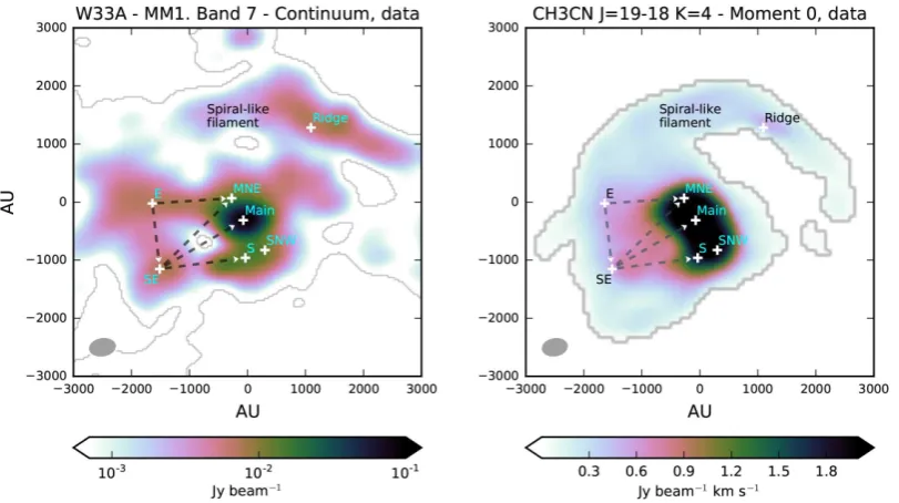
In Fig.1,we present the Band 7 continuum emission and the CH3CN J=19−18,K=4 moment 0 maps for the observational data. There, we highlight the compact sources as reported in Maud et al. (2017) and Galv´an-Madrid et al. (2010): Main, south (S), south-east (SE), east (E), and ridge. Two new compact sources are proposed in this paper and are labelled under the same rules: Main north-east (MNE) and south north-west (SNW), as well as five inter-source filaments represented with dashed lines, and the spiral-like filament in the northern part of the region.

The existence of MNE and SNW is mainly motivated by the CH3CN line emission. The moment 0 map evidences extended emission towards the north-east of Main and the north-west of S. This emission is also warm (see Maud et al.2017), and its veloc-ity field is more consistent with separate, redshifted blobs (see the last row of Fig.A1) than with a single, more extended source. For more details, see Section 4.1. On the other hand, the existence of inter-source filaments is motivated mostly by the extended features in the continuum maps that appear to join the compact sources (see Fig.1and Section 4.1.2), although some of these features are also apparent in the CH3CN maps.

3 M O D E L

3.1 Physical models

In order to describe this complex star formation region, we produce a global model made of the superposition of individual components, all within a 7000 au cubic region representing W33A MM1. In this section, we describe the physical attributes of the individual com-ponents. We emphasize that the final model is not unique nor a best fit, but it provides a reasonable match to the data and is physically motivated. The justification for the use and characteristics of each element are further explained in Sections 3.4, 3.5 and 4.

From the seven compact sources, four of them are disc-envelope systems (Main, S, SE, Ridge), two of them are pure rotating/infalling envelopes (MNE, SNW), corresponding to less evolved YSOs and one is a turbulent sphere (E), corresponding to an even younger object. Fig.2shows a schematic diagram of the relative positions and central masses of these sources.

3D radiative transfer modelling of W33A MM1

2507

Figure 1. Left: ALMA 349 GHz (0.8 mm) continuum image of W33A MM1. Right: velocity-integrated intensity (moment 0) of the CH3CN J=19−18, K=4 line data. Cells with intensity below 10 per cent of the peak were masked out. The compact sources included in the model are marked by crosses (+). The dashed arrows represent the modelled inter-source filaments and their flow direction. A label indicates the zone where the spiral-like filament resides. The beam size is shown in the lower left corner of the panels.

Figure 2. Configuration of compact sources and inter-source filaments in the W33A-MM1 model. Thex- andy-axes are parallel to RA and Dec. The

z-axis is parallel to the line of sight, with positive values increasing away from the observer. Thez=0 plane intersects the position of Main, and (x,

y)=(0, 0) coincides with the phase centre of the ALMA images. Arrows indicate the direction of the gas flows between sources. The sizes of the markers are related to the mass of the sources as shown in the top subplot.

filament which we interpret as an accretion flow feeding the centre of MM1 from its periphery, as proposed by Maud et al. (2017).

3.1.1 Compact sources

We implemented a standard YSO modelling for the four disc-envelope sources, following the approach of Keto & Zhang (2010). Those authors superpose a rotationally supported flared disc em-bedded in an infalling and rotating envelope. The envelope is mod-elled using the prescription of Ulrich (1976), who constructs the density and velocity fields assuming that the particles around the

stellar source follow ballistic paths. Although simple, this model has been useful to reproduce observations from the scales of low-mass (proto)stars up to high-low-mass clusters (e.g. Whitney et al.2003; Keto2007; Maud et al.2013).

For the envelope density, we use equation (1) of Keto & Zhang (2010):

ρenv(r, θ)=ρe0(r/Rd)−3/2

1+ cosθ

cosθ0

−1/2

×[1+(r/Rd)−1(3 cos2θ0−1)]−1, (1)

whereris the distance to the centre of the model andθ the polar angle;Rdis the centrifugal radius, defined as an equilibrium zone where the gravitational force of the central-point mass is equal to the centrifugal force of the rotating envelope;θ0is the initial angle of the streamline andρe0is the envelope normalization density at r =Rdandθ = π/2. They must satisfy the geometrical relation [equation (2) of Keto & Zhang2010]:

r = Rdcosθ0sin

2_θ 0 cosθ0−cosθ

. (2)

This constraint can be used to find an analytical expression for cosθ0(see its functional form in equation (13) of Mendoza, Cant´o & Raga2004).

The velocity components of the envelope are (see equations 14– 16 of Keto & Zhang2010):

vr(r, θ)= −

GM⋆

r

1/2

1+ cosθ

cosθ0

1/2

, (3)

vθ(r, θ)=

GM⋆

r

1/2

cosθ0−cosθ sinθ

1/2

1+ cosθ

cosθ0

1/2

,

(4)

vφ(r, θ)=

GM⋆

r

1/2 sinθ0

sinθ

1− cosθ

cosθ0

1/2

For the temperature of the envelope we follow Whitney et al. (2003) and assumeTenv(r)∝r−0.33. The proportionality constant is left as a free parameter to adjust density weighted mean tempera-tures according to the observational data.

We include the possibility of adding a conical cavity with an arbitrary opening angle.

For the disc, we implemented the standard prescription by Pringle (1981). We assume a steady, Keplerian, flared disc limited within the centrifugal radiusRdof the envelope. The disc density field is given by equation (3.14) of Pringle (1981):

ρdisc(z, R)=ρ0(R) exp{−z2/2H2(R)}, (6)

whereRandzare cylindrical coordinates.H(R) is the scale height of the disc andρ0(R) is the disc density function in the mid-plane (equations 7 and 8 of Keto & Zhang2010):

H(R)=H0(R/R⋆)1.25, (6a)

ρ0(R)=Aρρe0(Rd/R)2.25. (6b)

The scale height at the stellar radius is set toH0=0.01R⋆, and Aρis the density factor between disc and envelope atRd. The disc velocity is (equation 3.3 of Pringle1981):

v_disc=GM_⋆/R φ,ˆ (7) and the temperature (equation 12 f Keto & Zhang2010):

Tdisc=BT

3GM⋆M˙

4πR3σ

1−

R⋆

R

1/4

, (8)

whereBT is a factor to adjust disc heating and ˙M is the mass accretion rate given by equation (3) of Keto & Zhang (2010):

˙

M=ρe04πR

2

dvk, (9)

wherevkis the Keplerian velocity atRd.

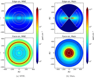
Fig.3shows the density and temperature structure of example disc and envelope models.

3.1.2 Accretion filaments

Elongated features joining some pairs of compact sources are ap-parent in the continuum images and in the line cubes (see Section 4). We modelled them as ‘accretion filaments’. Most of them are im-plemented as straight cylinders of∼103_{au length that join pairs of} compact sources, and with uniform density and temperature. The accompanying code leaves open the option of adding a dependency of density and temperature with cylindrical radius. We assume the kinetic energy of the filaments is related to their gravitational po-tential energy as given by the virial theorem:

3 5 GM⋆ r = 1 2v 2 , (10)

from which we obtain the speed at each point of the model. The main axis of each cylinder is defined asrcyl−ax=r⋆>−r⋆<, where r⋆>andr_⋆<are the positions of the most and least massive compact object in each pair. Additionally, we consider that the gravitational potential is fully determined by the most massive of the pair of sources and that the velocity in the cylinder points towards that source. This is analogous to considering that the entire gas inside the filament is within the Hill radius of the most massive compact source. The velocity field for each cylinder can be written as:

v_cyl(r)=

6GM⋆> 5

1/2

r−r⋆>

|r−r⋆>|3/2

. (11)

Since our simplifying assumptions imply that the most massive compact source is taking material from the least massive one, we fixed the systemic (initial) velocity of the flows to be the same as that of the low mass source in each pair. Note that the previous assumptions automatically fix the relative orientation of compact sources in thez-axis (line of sight).

There are five filamentary flows between pairs of compact sources in our model: SE→S, SE→Main, SE→MNE, E→MNE and E→SE (see Fig.2).

Additionally to the small cylindrical filaments, we include a larger (7240 au length) accretion filament reaching the central part of MM1 from its north side, following the interpretation of Maud et al. (2017) that this spiral-like structure is a ‘feeding filament’ that deposits material to the central region of MM1. We model the feeding filament structure using a parabolic cylinder with focus at the centre of mass of the entire region.

The speed along the parabolic trajectory is given by orbital energy conservation, and we also include a velocity component of collapse towards the axis of the parabolic filament. Thus, the vector velocity is

v_par(_r)=

2GMc

|r−rcm|

1/2

ˆ

t+vinn,ˆ (12)

where ˆtand ˆnare the tangent and normal unitary vectors associated to the main axis of the parabola. We set the infall velocity (vin) within the parabolic filament in terms of the speed of sound in the medium:cs = (γkBT/2mH)1/2, whereγ is the characteristic heat capacity ratio of the medium,kBthe Boltzmann constant andmH the Hydrogen mass. More details can be found in Section 4.1.2.

For simplicity, we set the density and temperature of the filaments to be homogeneous in each of them.

3.2 The model grids

3.2.1 Global grid

We create a global grid that harbors the individual local grids

(models) together. Each local grid is rotated and translated within the global grid according to the restrictions given by observational data. The global grid is homogeneous and cubic: it has 301 nodes distributed in equal steps over 7000 au in each direction, i.e. it is built with∼27×106_{points, and its linear resolution is 23.3 au.} Fig.4shows a visualization of the final global grid where the density of plotted points is proportional to the model density.

To overlap thelocal gridswithin the global grid, an algorithm for distance minimization between the nodes of both was made. Thus, spatial information is extracted from each node of each local grid and the corresponding nearest node in the global grid is found. This point will inherit the physical properties that the local grid point was saving. Since local grids aregenerally more spatially resolved than the global grid, it is likely to occur that some cells of

a givenlocal grid converge to the same closest node in the global grid. When this happens, the latter node takes the average of the overlapping densities. Other properties are taken as their density-weighted averages.

3D radiative transfer modelling of W33A MM1

2509

Figure 3. (a) Left: density (colours) and temperature (contours) profiles for a pure (Ulrich) envelope compact source. The example corresponds to the final model for MNE. (b) Right: density and temperature profiles for a compact source made of a disc plus an envelope. The example corresponds to Main, which has a cavity. The top subplots show the edge-on (i=90◦_{) middle cut of the models, and the bottom subplots show the face-on (i=0}◦_{) middle cut.}

Figure 4. Visualization of the global grid, which is made of the superposi-tion of many local grids, each representing an individual submodel. Regions with a higher density of points have a larger mass density in the model. Colours indicate the depth in thez-axis, with positive values increasing away from the observer. The z=0 plane intersects the position of Main, and (x,y)=(0, 0) coincides with the phase centre of the ALMA images.

3.2.2 Local grids

For the compact sources, each local grid was also set to be homoge-neous in Cartesian coordinates. These local grids can have different physical sizes and resolutions each.

For the models containing an Ulrich envelope, we added a condi-tion to ensure that no point of their grids falls into the mathematically undefined position (r,θ)=(Rd,π/2), where the density diverges. The interpretation of this jump in density is that the ‘true’ disc starts inwards (Mendoza et al.2004).

For the cylinders, the nodes of their local grids are evenly and randomly distributed. To do so, we first generate a random point along the axis of the cylinder. Secondly, we create a vector with fixed position in that point, with random orientation (restricted to be perpendicular to the axis) and length in the ranges [0, 2π] and [0,Rcyl], respectively. This recipe is repeated (2Rcyl)2|rcyl−ax|/dr3 times to ensure that all the cells of the global grid enclosed by the virtual cylindrical surface will have enough points around them to be filled with.dris the maximum possible separation between neighbouring nodes in the global grid:dr=dx2_+dy2_+dz2_.

The grid of the parabolic filament was built in a similar way to those of the cylinders, with an extra consideration due to the curved trajectory. First, we consider the characteristic equation of a parabola isx2_{=4py, wherepis the parameter that accounts for its} focus. Then, it is possible to calculate all the tangent vectors in the parabolic section of analysis as follows:

ˆ

t=cos(θ)ˆi+sin(θ) ˆj ,

θ(x)=tan−1_(x/2p), (13)

repeat this step enough times to populate correctly this zone in the global grid, as explained in the previous paragraph.

3.3 Radiative transfer simulations

We use version 1.6.1 of the Line Modelling Engine code (LIME, Brinch & Hogerheijde2010) to perform radiative transfer simula-tions of the physical grids described in the previous section.LIME calculates both molecular line and (dust) continuum maps by solv-ing the molecular excitation or fixsolv-ing it in the LTE case, and then the transfer of radiation through the model. It builds unstructured 3D Delaunay grids by generating a set of random points across the domain that will be accepted or rejected according to the density of the given model. Then, the grid is smoothed via Voronoi tessel-lations.LIMEretrieves molecular data from the LAMDA data base (Sch¨oier et al.2005).

A few adaptations had to be made to be able to feed our models intoLIME. The necessary code is available through the GitHub link provided in Appendix B. We included a header script inLIMEto upload the output data from our model-generating codes. Also, we added in the user interface script (model.c) an algorithm to determine the nearest neighbours between the randomly generated set of points inLIMEand the points of our global grid, following the suggestions made in theLIMEdocumentation.1Given that our grid is homogeneous in Cartesian coordinates, it is possible to efficiently determine the closest pairs of points. Let us call a random generated LIMEpoint (xr,yr,zr) and its nearest point in our grid (xm,ym,zm). First, we compute the nearestyzplane associated with the givenxr, so,xmis found. Then, in that plane we look for the nearest column associated with the givenyr, soymis found. Finally, in that column we compute the nearest cell associated with the givenzr, sozmis found. In the end, the point (xr,yr,zr) receives all the properties belonging to (xm,ym,zm).

The rotational (J,K) transitions of CH3CN are such that several

Klines for a given J + 1→J can be observed in a single spectral set-up (e.g. Cummins et al.1983; Remijan et al.2004). This fact has made these lines a widely used tracer of warm, dense gas (e.g. Araya et al.2005; Purcell et al.2006; Cesaroni et al.2017). We use LTE calculations for our modelling. This is justified since the critical density of the J=19−18,K=4, andK=8 transitions at the model temperatures isncrit≈1×107cm−3. Also, ‘effective’ densities for thermalization are typically at least one order of magnitude below critical densities (Evans1999). Most of the mass in our domain is above the critical density of the modelled lines.

We allow for different CH3CN abundances with respect to H2for each submodel (see Section 3.5). The gas-to-dust mass ratio was set to 100 in the entire global grid.

Some fluctuations in the model continuum emission appear be-cause the grid points randomly generated byLIME2do not map the region completely, since they are fewer than the model grid points. Therefore, different model regions are better covered withLIMEgrid points in some runs than in others. To smooth these fluctuations, for each continuum image presented in this paper, we generated 10 images with the same set of parameters. Then we extracted the median of the intensity for each pixel and constructed a final image. This averaging process is equivalent to generate an image with a higher number of grid points inLIME, but faster. We found that the

1_{http://lime.readthedocs.io/en/latest, section Advanced set-up.} 2_{Defined with the ‘pIntensity’ parameter.}

line emission is not sensitive to this effect because it is brighter than the continuum, so the fluctuations are not noticeable.

Finally, the output images and cubes created with LIME were passed through the ALMA instrumental response using version 4.4.0 of CASA (McMullin et al.2007). The task ‘simobserve’ was first used to generate visibilities from the model images. The array configuration, integration time, date, hour angle and precipitable water vapor were all set to properly emulate the observing con-ditions of the data. The task ‘clean’ was then used to create the ALMA-simulated images from the model visibilities. The simu-lated and observed images have noise levels and beam sizes match-ing each other within a few per cent.

3.4 Iterative building of global model

In this section, we summarize the order in which the global model was tailored and the motivation for its specific features. Section 3.5 goes deeper into the determination of the free parameters of the local models.

We started modelling compact source Main with a single massive envelope, but in the end a disc embedded within an envelope was a better match to the data. Then, we proceeded to model compact sources S, SE, E, and Ridge. Each source was modelled separately in the same way as Main, in its own local grid. The top row of Fig.5illustrates the effects of changing the model prescription for compact source S on its CH3CN line profiles, modelled in isolation. More details can be found in Section 4.1.1.

The next step was to construct the global grid (Section 3.2.1) and allocate the compact sources within it. The first global grid contained only compact sources. This global model was compared to the observations, then the small inter-source filaments were de-fined and assigned to a second global grid. Small adjustments to the properties of the compact sources and small filaments were done by physically motivated trial and error to better match this second global grid to the observational data. The influence of the global en-vironment on the line profiles of source S can be seen in the bottom row of Fig.5.

The final addition to the global grid was the spiral-like filament feature. The assumption of a parabolic orbit with focus at the centre of mass of MM1 was readily a good approximation. Then, the 3D orientation and density of the parabola were adjusted to match the observed velocity gradient and fluxes. This filament was initially considered to be static, but a radial collapse component was added to better match its observed velocity dispersion and morphology in the channel maps (see Fig.A1).

Finally, the newly proposed compact sources MNE and SNW were added to reproduce finer features in the images. Their inclusion helped to reproduce the extended heating and velocity dispersion towards the north-east of Main and the north-west of South (S), as well as the secondary features around Main and S (more details below). In the resulting global grid, additional small adjustments to each component were tried until we were satisfied with the match between the global model and observations. We reiterate that the models are not best fits to the data, but a physically motivated representation that matches the observations reasonably well (e.g. Schmiedeke et al.2016).

3.5 Determination of model parameters

3D radiative transfer modelling of W33A MM1

2511

Figure 5. CH3CN J=19−18,K=4 (left) andK=8 (right) spectra for different isolated (top row) and global (bottom row) models for source S. The scenarios

are: disc-only (yellow line), envelope-only (red line) and disc + envelope (green line). The dashed lines in the bottom panels show the ALMA data. The rms noise levels in the spectra are∼1 K (see Section 2.)

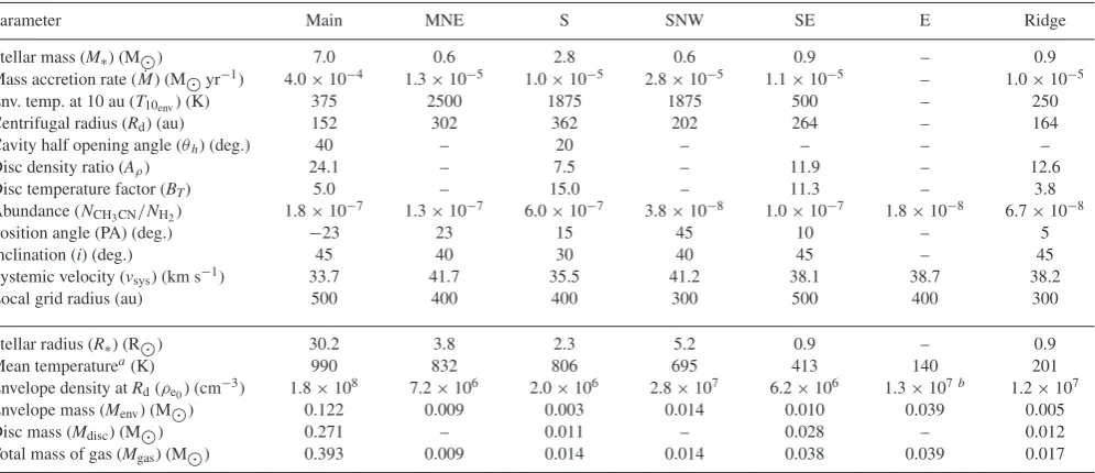
Table 1. Top: Free parameters for compact sources. Bottom: Derived properties from model output.

Parameter Main MNE S SNW SE E Ridge

Stellar mass (M∗) (M⊙) 7.0 0.6 2.8 0.6 0.9 – 0.9

Mass accretion rate ( ˙M) (M_⊙yr−1_{) 4.0×10}−4 _1.3×10−5 _1.0×10−5 _2.8×10−5 _1.1×10−5 _{– 1.0×10}−5

Env. temp. at 10 au (T10env) (K) 375 2500 1875 1875 500 – 250

Centrifugal radius (Rd) (au) 152 302 362 202 264 – 164

Cavity half opening angle (θh) (deg.) 40 – 20 – – – –

Disc density ratio (Aρ) 24.1 – 7.5 – 11.9 – 12.6

Disc temperature factor (BT) 5.0 – 15.0 – 11.3 – 3.8

Abundance (NCH3CN/NH2) 1.8×10−

7 _1.3×10−7 _6.0×10−7 _3.8×10−8 _1.0×10−7 _1.8×10−8 _6.7×10−8

Position angle (PA) (deg.) −23 23 15 45 10 – 5

Inclination (i) (deg.) 45 40 30 40 45 – 45

Systemic velocity (vsys) (km s−1) 33.7 41.7 35.5 41.2 38.1 38.7 38.2

Local grid radius (au) 500 400 400 300 500 400 300

Stellar radius (R∗) (R_⊙) 30.2 3.8 2.3 5.2 0.9 – 0.9

Mean temperaturea(K) 990 832 806 695 413 140 201

Envelope density atRd(ρe0) (cm

−3_{) 1.8×10}8 _7.2×106 _2.0×106 _2.8×107 _6.2×106 _1.3×107b _1.2×107

Envelope mass (Menv) (M_⊙) 0.122 0.009 0.003 0.014 0.010 0.039 0.005

Disc mass (Mdisc) (M_⊙) 0.271 – 0.011 – 0.028 – 0.012

Total mass of gas (Mgas) (M_⊙) 0.393 0.009 0.014 0.014 0.038 0.039 0.017

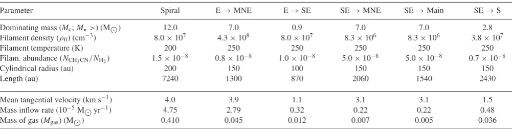
Table 2. Same as Table1but for the filamentary structures.

Parameter Spiral E→MNE E→SE SE→MNE SE→Main SE→S

Dominating mass (Mc;M⋆>) (M_⊙) 12.0 7.0 0.9 7.0 7.0 2.8

Filament density (ρ0) (cm−3) 8.0×107 4.3×108 8.0×107 8.3×106 8.3×106 3.8×107

Filament temperature (K) 200 250 250 250 250 250

Filam. abundance (NCH3CN/NH2) 1.5×10

−8 _0.8×10−8 _1.0×10−8 _5.0×10−8 _5.0×10−8 _0.7×10−8

Cylindrical radius (au) 200 150 100 150 150 150

Length (au) 7240 1300 870 2060 1540 2430

Mean tangential velocity (km s−1_{) 4.0 3.9 1.1 3.1 3.1 1.5}

Mass inflow rate (10−5_M

⊙yr−1) 4.75 2.79 0.32 0.22 0.22 0.48

Mass of gas (Mgas) (M_⊙) 0.410 0.045 0.012 0.007 0.005 0.036

were determined. We emphasize that our method was intuition-guided trial and error. To find a good set of parameters we iterated over different model versions mainly comparing their CH3CNK=4 and 0.8 mm continuum to the data, whereas theK=8 line and 1.3 mm continuum were just used asa posteriorichecks.

Although the central stellar massM⋆is not the unique parameter

that affects the line-width, it is the most important (see equations 3– 5 and 7). For a first estimation of the stellar mass of the compact sources, we first inspected the channel maps around their central positions as defined from the continuum peaks. In some compact sources, a velocity gradient was clearly discernible (S, SE, Ridge), while in some others it was not (Main, MNE, SNW), probably due to the confusion with neighbouring emission. For the sources with clear velocity gradients, we extracted their spectra averaged over the relevant apertures and made Gaussian fits to obtain estimations of the projected rotation velocity of the gas ( v=0.5FWHM), while estimating the disc radiusrfrom measuring the angular separation between the blue- and redshifted emission lobes. Using these pa-rameters, we made a first estimation of the central mass assuming Keplerian rotation as inM⋆= v2r/G. For the sources without clear

velocity gradients in the channel maps, we estimated their stellar mass by matching the full width at half-maximum (FWHM) of the modelled CH3CN line with the data in the central beam of each. For the case of Main, we started with the 13 M_⊙estimation from Maud et al. (2017), and reduced it down to 7 M_⊙due to our interpretation of multiplicity (see Section 4.1.1 for more details).

After their first estimation, the central masses were slightly varied to better match the data. The inclinationiwith respect to the line of sight is also important and is the second preferred parameter that we vary to adjust line-widths. For Main, we used the previous estimate based on models by de Wit et al. (2010), whereas for the other sources we started with the assumption ofi=45◦_{and varied}

it until we achieved a line-width that matched the observed. A cavity with opening half-angleθhwas included in the models of

Main and S. Observations show that MM1 has at least one molecular outflow centred in Main (Davies et al.2010; Galv´an-Madrid et al.

2010). It is not clear whether S also drives an outflow, but we incorporated a cavity in its model given that it is the second most massive source. The cavity was used mainly to refine the line profile of these sources but also to construct a more realistic model of their inner regions. We variedθh from 0◦ to 80◦in steps of 20◦ (see

Fig.6).

The mass accretion rate ˙M was varied as a free parameter in order to scale up or down the density of the compact sources, with a corresponding effect on the line and continuum intensity levels. From equation (9), the normalization constantρe0of the envelope

density is directly proportional to ˙M. Note that as a consequence,

this is also true for the disc density (see equation 6b). Since Main is a high-mass protostellar object, we used ˙Min the range 10−4_to 10−3_M

⊙yr−1(e.g. Zinnecker & Yorke2007; Osorio et al.2009).

For the lower mass sources, we tested values in the range 10−6_to 10−5_M

⊙yr−1.

The normalization of the envelope temperature and the disc tem-perature factorBTwas set such that the resultant density weighted mean temperature of the compact sources was consistent with the temperature map presented in Maud et al. (2017). Similarly, the disc density ratioAρis used to calibrate the density-weighted mean

temperature, as well as the continuum and line intensities, with the observational data. We restrict both parametersBTandAρto values ∼5–20, in order to not exaggerate the relative importance of the disc with respect to the envelope.

The centrifugal radius of the envelopeRdwas chosen to be the same disc radius previously defined in this section. The line emis-sion of MNE and SNW is marginally (un)resolved; thus, we re-strictedRdto be larger than half of the envelope size. The emission in Main is quite compact, so we set Rdfrom the line-width and continuum intensity in its central beam. The PA in the plane of the sky was also defined from the same restrictions asRd. For Main, previous observations and modelling provided a good first estimate (de Wit et al.2010; Davies et al.2010).

For the CH3CN abundance with respect to H2,NCH3CN/H2, we

tested values from 10−9_{to 10}−7_{, in agreement with determinations} using interferometric observations in massive star formation re-gions (e.g. Wilner, Wright & Plambeck1994; Remijan et al.2004; Galv´an-Madrid et al.2009). We started withNCH3CN/H2 = 10

−9

and increased it in order to adjust the line emission once the correct continuum flux was achieved.

The systemic velocityvsysof the compact sources was set to be the velocity of the line peak in the data. For cases like Main where theK=4 CH3CN line was optically thick at the centre, theK=8 line was also considered to refinevsys.

The dominating mass is the mass responsible for the gravita-tional field that determines the gas velocity in the filaments (see equations 11 and 12). For the large parabolic filament, the dominat-ing mass is set to the total model mass contained in the central region of MM1, i.e. stellar + gas mass of Main + S + MNE + SNW + the gaseous mass in their vicinity. For the cylindrical filaments con-verging to Main or MNE, the dominating mass is the mass of Main. For the rest of the small filaments, it is the mass of the most massive of the two sources at the extremes of the cylinder.

3D radiative transfer modelling of W33A MM1

2513

Figure 6. Effect of varying the cavity opening angle on the spectra of compact source Main modelled in isolation. The upper row shows from left to right:

θh=0◦, 20◦, 40◦. The bottom row showsθh=60◦(left) andθh=80◦(right). The middle panel of the bottom row shows the resulting CH3CN J=19−18, K=4 spectra. Density (colours) and temperature (contours) profiles were also included in the subplots. The cross-sections show edge-on models (i=90◦_). The spectra come from models with inclinationi=45◦_{, the same as Main in the model. It is clear that the two-peaked profile is only seen with cavities wider} than 60◦_{when the disc dominates the emission.}

mainly to control the continuum intensity, whereas the CH3CN abundance was used to further adjust the line emission. We tested H2particle densities from 106to 108cm−3and abundances from 10−9_{to 10}−7_.

The length of the filaments was estimated from the spatial con-figuration of the compact sources in the data. We assume that the cylinders have the same depth in the line of sight as projected length in the plane of the sky (see Section 4.1.2 for further details). The cylindrical radii were estimated directly from the apparent angular width of the filaments in the continuum and channel maps.

4 R E S U LT S

4.1 CH3CN J=19–18,K=4

4.1.1 Compact sources

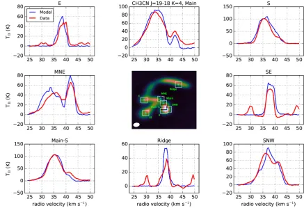
To compare the model spectra of the compact sources with those from the ALMA images, in Fig.7we show the average spectra in squared apertures of 0.2 arcsec size (approximately the beam size). The observed lines are generally asymmetric, and in most cases there are secondary velocity features besides the principal line peaks. The presence of such features in apertures already as small as 480 au, as well as the absence of pure two-peaked line profiles, warns against interpreting the compact sources only as Keplerian, rotationally supported discs. Nearby companions, envelopes and filamentary flows can all contribute to the observed spectra.

The spectrum around compact source Main consists of a single-peaked line centred at∼34 km s−1_{, and a secondary, fainter} compo-nent peaked at∼42 km s−1_{(see Fig.7). In our model, the brightest} line peak is dominated by Main, whereas the redshifted, fainter spectral component is contributed by compact source MNE. Our interpretation also reproduces the spectrum around the central po-sition of MNE.

To model Main we first considered the simplest case of a pure Keplerian disc, but such model always produces double-peaked profiles unless an unrealistically high optical depth – mass – is used, which consequently also produces line and continuum fluxes that are too high. We concluded that an envelope surrounding the disc is the most natural way to produce the single-peaked profile of the brightest spectral component (see Fig.7) while matching both theK=4 and continuum fluxes. The inclination angle was chosen based on the restrictions available from the IR interferometric and photometric modelling of de Wit et al. (2010), who foundi∼50◦

(we seti=45◦_{for simplicity). Several observations show that Main}

drives one, or possibly two massive molecular outflows (Davies et al. 2010; Galv´an-Madrid et al.2010; Maud et al. 2015) and possess a cavity on scales of a few×100 au (de Wit et al.2010). We included such cavity in the model. Fig.6shows the effect of changing the opening angle of the cavity on the model spectra of Main. An opening angleθ=40◦_{is a good compromise between}

Figure 7. CH3CN J=19−18,K=4 spectra of the modelled compact sources compared with the data. The header on each panel indicates the region of

analysis. The central panel is a snapshot of the velocity channelv=38.05 km s−1_{, where the 0.2×0.2 arcsec integration apertures around compact sources are}

marked in white. The dashed line apertures are centred in the new compact sources proposed by the model (MNE and SNW). The black square shows an extra aperture of interest in between compact sources Main and S, labelled as Main-S in the spectra. The cyan markers indicate the centre of the compact sources included in the model.

Although Main is still the most massive object in the field (the full list of free parameters and derived quantities is in Table1), we determined a lower central mass and smaller disc size than previous estimates. In previous (sub)mm observations where the entire MM1 core3_{was marginally resolved, the kinematics was interpreted as} originating from a dynamical mass of 10–15M_⊙within an∼1200 au radius (Galv´an-Madrid et al.2010). Maud et al. (2017) deter-mined a dynamical mass∼13 M_⊙within a 1000 au radius from the current ALMA data. Given that we interpret emission peaks MNE, SNW and S asseparateYSOs, and also consider several filamen-tary flows feeding Main, MNE and S from the east and south-east, our model of Main requires a lower stellar mass (7 M_⊙), dynamical mass (stellar + disc + envelope, 7.4 M_⊙), and disc radius (∼150 au) than previous estimates. The total stellar + gas mass of our model within a 1000 au radius of the stellar source in Main is∼12 M_⊙, consistent with previous estimates. The 150 au disc radius that we propose for Main is unresolved by our observations with 400 au resolution, but ALMA long-baseline data will be able to test our hypothesis or discard the existence of atrue discon scales<100 au.

For compact source S, as for the case of Main, the observed pro-file is not a simple two-peaked line. In this case there is a dominant

3_{We refer to MM1 as a ‘core’ following the convention of using this word for}

structures of∼0.03–0.2 pc size (e.g. Bergin & Tafalla2007). The individual discs and envelopes in our model are smaller scale structures within the MM1 core.

peak at∼36 km s−1_{, with a fainter, redshifted shoulder from∼40 to} 44 km s−1_{, which in our model comes from the neighbouring} com-pact source SNW (see below). Fig.5shows a comparison of the CH3CN J=19−18,K=4, andK=8 lines for source S resulting from three model scenarios: an envelope without disc, a disc without envelope, and a disc + envelope. The line profile of the pure enve-lope, and more prominently, of the pure disc, have the two peaks characteristic of rotation, whereas in the disc + envelope model the peaks are much less noticeable. To reach the desired peak intensity at theK=4 transition, we scaled up the density through increasing the mass accretion rate in the different model scenarios. A pure envelope needs to become too optically thick over a wide velocity range, in which case the line is too ‘square-shaped’. Similarly, a pure disc does not preserve the desired peak intensity at theK=8 transition. Regarding to the continuum emission, the pure envelope has low mean and peak intensities (∼1/5 compared to the data at 349 GHz), whereas the pure disc generates intensities that are too high by×4. Moreover, only the disc + envelope model shows a line profile similar to the data in both transitions while maintaining the correct continuum intensities. Thus, we concluded that a disc + en-velope is the best model for source S. We included a cavity in this model too, given that S is the second most massive source. After spanning the possible range of values for the inclination angle with respect to the line of sightiand the cavity half-opening angleθh, we

found thati=30◦_{(closer to face-on than to edge-on) andθ} h=20◦

3D radiative transfer modelling of W33A MM1

2515

Two small peaks close to Main and S are reproduced by including two new compact sources, which we label Main NE (MNE) and South NW (SNW). The emission from these objects is reproduced by considering two low-mass sources with a central mass of 0.6 M_⊙ surrounded by a pure Ulrich envelope. The model spectrum of SNW has a significant contribution from the nearby, brighter source S. Similarly, the spectrum of MNE is influenced by the contribution from Main (see Fig.7).

Compact source SE is modelled as a disc + envelope system, in a similar way to Main and S. There are no previous constraints on its disc inclination, so we decided to set it to 45◦_{. The model}

reproduces the principal line peak at∼38 km s−1_{, but does not} re-produce the fainter blue- and redshifted components (Fig.7), which likely arise from contamination of neighbouring molecular lines. This contamination is also apparent at similar velocity ranges in the spectra around compact sources E and Ridge, all of them related to the larger spiral-like filament.

Compact sourceEdoes not have any evidence of velocity gradi-ents in the observational cubes. Therefore, we decided to model it as a sphere with a power-law density profile and a random velocity distribution. The velocity dispersion was chosen to reproduce the observed line-width. This source probably represents a younger, lower mass, pre-stellar core.

Compact sourceRidgeis embedded within the spiral-like filament before it reaches the crowded central part of MM1. Its relatively high brightness and velocity dispersion motivated us to model it as a disc-envelope system rather than just a turbulent sphere as was the case for source E. The model line is brighter and narrower than in the data, but still matches them reasonably.

We also show in Fig.7the zone between Main and S, labelled as Main-S. In the model, the spectrum of Main-S has contribu-tions from three compact sources: Main, S and SNW. The good match illustrates that our model is a reasonable approximation of the observed system. Table1lists the final model parameters for the compact sources.

4.1.2 Accretion filaments

Two types of accretion filaments are included in our global model of W33A MM1 (see Section 3.1.2): a larger spiral-like filament feeding MM1 from the outside, and smaller, straight filaments joining pairs of compact sources. Table 2lists the parameters of the selected models.

Fig. 8 shows the moment maps (velocity integrated intensity, intensity-weighted mean velocity, and intensity weighted veloc-ity dispersion) of the model and the observational data. It is seen that thespiral-like ‘feeding’ filamentmodel is a good description of the observations. This filament approaches the central part of MM1 coming from the near, north-west side of the observer, and moves towards the east and away from the observer, to finally turn towards the observer while merging with MM1 close to compact source E. We emphasize that the model is physically motivated, since the velocity field was calculated assuming test particles that approach from the infinite at rest and follow a parabolic trajectory in which the mass of the central region of MM1 resides at its fo-cus. This simple prescription naturally reproduces the blueshifted– redshifted–blueshifted pattern of the line-of-sight velocity across the filament as projected on to the plane of the sky. The real fila-ment seems somewhat more closed and extended than the model in its far end, something that a purely parabolic trajectory cannot reproduce. In spite of being quite warm (200 K), an extra velocity

component was needed to reproduce the observed velocity disper-sion along the trajectory of this filament. We therefore implemented the reasonable assumption that the filament has radial, transonic collapse. Withγ =7/5 (diatomic molecules) we set a radial infall velocity vin= 1.5cs=1.6 km s−1 (see Section 3.1.2), something in between the subsonic and supersonic collapse observed towards low- and high-mass star-forming cores, respectively (e.g. Galv´an-Madrid et al.2009; Keto, Caselli & Rawlings2015). Adding this radial component increased the velocity dispersion to levels close to the observed, although still slightly below. Fig.9shows a com-parison of the model and observed spectra in an aperture containing the entire spiral-like filament.

The small (length∼103_{au) cylindrical filaments are required to} reproduce the elongated emission joints observed between compact sources in the line emission maps and the (sub)mm continuum (see Section 4.2). Again, the models are physically plausible since we consider that the gas follows Newtonian dynamics and go from the less massive object to the more massive one. Their length in the line-of-sight direction is considered to be the same as their projected size in the plane of the sky. Two such flows go from compact source E to SE and MNE, and three more go from compact source SE to Main, S, and MNE. Table2lists the selected parameters of these five filaments. The existence of the two filaments that cross diagonally (SE→Main and SE→MNE) is not clear, but including them helped to reproduce line emission extending towards the north-west of compact source SE. Figs8andA1show that the model cylinders fill the gaps of emission at the centre of MM1, and that they also help to reproduce the velocity dispersion between compact sources. Our small model filaments are homogeneous and do not reproduce the clumpiness suggested by the data.

Something worth noting is that fixing the starting and ending point of the cylindrical flows, plus the above-mentioned dynamical initial condition, automatically sets the line-of-sight arrangement of sources, allowing us to fully determine the 3D structure of the model cluster.

4.1.3 The entire W33A MM1 region

Figure 8. Top row: intensity moments for the model CH3CN J=19−18,K=4 line. Left: velocity-integrated intensity (moment 0). Centre:intensity-weighted

mean velocity (moment 1) integrated between 25.0 and 49.8 km s−1_{. Right: intensity-weighted velocity dispersion (σ, moment 2) over the same integration}

range as the moment 1. Bottom row: same as top row but for the ALMA data. Cells with intensity below 10 per cent of the peak were masked out. The compact sources included in the model are marked by crosses (+). The beam is shown in the lower left corner of top left panel.

molecular lines within the velocity integration range for these two sources (see Fig.7).

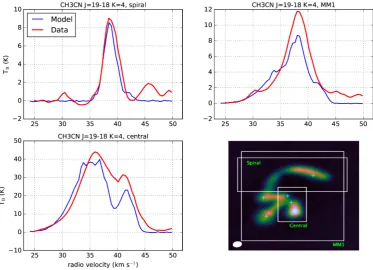
Fig.9shows a comparison of the model and observed spectra averaged in larger apertures containing the entire MM1 core and a region covering the brightest emission (Main + MNE + S + SNW), labelled as ‘central’. In the former, it is clear that the model repro-duces the line centroid and width but is lacking about one-third of the peak aperture-averaged brightness temperature, i.e. the missing extended emission mentioned above. The match of the model in the ‘central’ part is better, although still some brightness from extended emission is missing. Appendix A shows the channel maps of both the model and ALMA data for further comparison. It is also clear from these that some extended emission is missing in the model, but that such emission could not be modelled with a core-scale, Ulrich-type or spherical envelope.

4.2 (Sub)millimetre dust continuum

Model continuum maps of the thermal dust emission at 220.8 GHz (1.36 mm) and 349.3 GHz (0.86 mm) and the corresponding ALMA maps are shown together in Fig.10. We use an opacity power-law

κ=κ0(ν/ν0)β with an opacity indexβ=1.7, typical of the ISM, and a normalizationκ0=0.5 cm2g−1at 220 GHz as in Galv´an-Madrid et al. (2010). The global model was chosen to match well

the 0.86 mm continuum and CH3CN J=19−18 line, and then the resulting 1.36 mm flux is calculated.

In Table3, we list the peak and averaged continuum intensities over the same apertures used for the line analysis (Figs7and9). We avoid quoting fluxes4_{for the following reasons: (i) The Band 7} and Band 6 beams are about and larger than the 0.2 arcsec apertures that we use for the compact sources, respectively, and the sources are also of the order of this size. Thus, fluxes measured over these apertures do not exactly correspond to the correct source flux. (ii) In some cases there is crowding between the compact sources and also with the filaments. Selecting larger apertures compared to the beam would help to solve the previous point (i), but then the fluxes do not correspond anymore to those from individual objects. Selecting smaller apertures helps to isolate individual sources, but the situation of point (i) gets worse.

For compact source Main, we found that a disc is needed to match the high and compact continuum intensities. Without a disc, a pure envelope only produces∼10 per cent of the needed continuum emis-sion, and its appearance is more extended than in the observations. This is a natural consequence of the envelope being less compact

4_{Throughout this paper, we use the word ‘flux’ to refer to a flux density,}

3D radiative transfer modelling of W33A MM1

2517

Figure 9. CH3CN J=19−18,K=4 line emission of model and ALMA data compared in large apertures of interest. The header on each panel indicates the

zone of analysis. The bottom right-hand panel is a snapshot of the cube in the velocity channelv=38.05 km s−1_{, where white squares show the areas over}

which the spectra have been averaged. The cyan markers indicate the centre of the compact sources included in the model.

than the disc (see Fig.3). Also, the compact appearance of the con-tinuum and the line data suggests that the disc around Main should be small. Table1shows that the estimated disc radius (152 au) is the smallest among all sources.

A disc is also necessary to match the continuum emission of compact sources S, SE, and Ridge. For S, the mean intensity is dominated by the disc, with important contributions from the SE→S filament and the close companion SNW. These external agents help to reproduce the horizontally elongated continuum emission in Band 7 around S (see Fig.10). The mean intensity in SE has a significant contribution from the three filamentary flows coming/going from/to other sources. Source Ridge alters the appearance of the spiral-like filament, and a disc is needed to match the observational data. On the other hand, MNE and SNW are not required to host discs to reproduce their observed continuum.

The mean intensity of the model spiral-like filament matches well the observations in both bands, but the real emission has inhomo-geneities besides compact source Ridge that are not included in the model. An increased density towards Ridge would improve the match.

The need for the filamentary flows joining pairs of compact sources is apparent in the continuum images. The bright, elon-gated features in the middle zones between compact sources are well reproduced by the global model thanks to the inclusion of the cylindrical filaments. Similarly to the case of the line emission, the model lacks some extended emission that could arise from core emission not belonging to any of the compact sources or filaments. This extended emission, although morphologically noticeable in the real observations, amounts to only 22 per cent and 10 per cent flux on top of what the model, respectively, has at 1.3 and 0.8 mm, which is within the nominal 10 per cent error in the observational flux determinations.

Spectral indices were calculated for the large apertures shown in Fig. 9. The model integrated fluxes for the spiral-like filament, the central-MM1 region, and the entire MM1 core, respectively, at 1.3 and 0.8 mm are: Sspiral,1.3mm = 30.0 mJy,

Sspiral,0.8mm = 85.6 mJy, Scentral,1.3mm = 51.1 mJy,

Scentral,0.8mm = 194.0 mJy, SMM1,1.3mm = 102.4 mJy, and

SMM1,0.8mm = 320.6 mJy. The respective fluxes in the ALMA data are: Sspiral,1.3mm = 34.0 mJy, Sspiral,0.8mm = 85.2 mJy,

Scentral,1.3mm = 71.1 mJy, Scentral,0.8mm = 203.0 mJy,

SMM1,1.3mm = 125.0 mJy, and SMM1,0.8mm = 341.1 mJy. The free–free contributions were subtracted from the observational data extrapolating the fluxes of the 7 mm sources in van der Tak & Menten (2005) and using a free–free spectral index of 1 (see also Maud et al.2017; Galv´an-Madrid et al.2010). Thus, the obtained model dust spectral indices are: αspiral = 2.3,αcentral = 2.9, and

αMM1=2.5. The observational spectral indices are:αspiral =2.0,

αcentral=2.3, andαMM1=2.2. The observational indices appear to be systematically lower than in the model, but taking into account the absolute uncertainties of about 10 per cent for both sets of images, the associated error in the spectral index calculation is

±0.3, which makes the model and ALMA measurements consistent with each other.

We note that the measured spectral indices in the model do not correspond to the 2 + β that is often expected, and that is valid only under the Rayleigh–Jeans approximation and the optically thin regime (e.g. Maud et al.2013). Optical depth maps show that the model regions are optically thin on average except for the central parts of Main and SE, where the mean τ > 0.5. Therefore, we interpret the low spectral indices as due to significant portions of the model being out of the Rayleigh–Jeans regime:hνis in general less thankT, but not much less over large volumes. For example

Figure 10. 220 GHz (left column) and 349 GHz (right column) continuum images of W33A MM1. Top panels correspond to the model and bottom panels to the observations. The compact sources included in the model are marked with crosses (+). The beam is shown in the lower left corner of each panel. The colour bars are shared between panels of the same column.

Table 3. Mean and peak continuum intensities of the modelled and observed regions. The known free–free contributions from Main and SE were extracted in Main, SE, central-MM1, and MM1 for the data. The measurement apertures are the same as in Figs7and9except for SE, where we used a larger aperture to subtract adequately the free–free contribution. The absolute uncertainties are≈10 per cent for both models and observations.

Region Model Data

220 GHz 220 GHz 349 GHz 349 GHz 220 GHz 220 GHz 349 GHz 349 GHz

Mean (mJy beam−1)

Peak (mJy beam−1)

Mean (mJy beam−1)

Peak (mJy beam−1)

Mean (mJy beam−1)

Peak (mJy beam−1)

Mean (mJy beam−1)

Peak (mJy beam−1)

Main 26.2 33.6 67.3 119.7 25.0 44.9 56.8 96.9

MNE 10.8 29.8 19.4 79.1 18.6 49.4 18.1 65.8

S 5.7 15.0 9.0 15.0 12.2 23.6 12.7 16.3

SNW 4.6 18.4 9.7 25.8 11.1 30.7 11.5 24.4

SE 1.0 2.1 3.6 12.7 2.0 1.8 3.6 7.9

E 2.1 2.9 8.5 14.5 5.1 5.5 6.4 7.7

Ridge 1.4 1.9 6.6 10.3 3.6 4.7 5.9 8.0

Main-S 17.9 32.9 33.4 110.2 28.8 50.4 30.2 87.9

Spiral 0.5 3.3 1.6 10.9 1.5 8.9 1.4 8.7

Central-MM1 6.3 33.6 11.7 119.7 11.4 44.9 12.3 96.9

3D radiative transfer modelling of W33A MM1

2519

of MM1 has an elevated optical depth, it is the closest to following the Rayleigh–Jeans limit, given that the temperatures there are also substantially higher. It is possible that the origin of the low spectral indices in the real ALMA maps is the same, warning against readily interpreting low dust-emission spectral indices as a signature of grain growth when observations at frequencies larger than 300 GHz are used.

4.3 CH3CN J=19−18,K =8

We now present a calculation of the CH3CN J= 19−18,K=8 line based on the previously described global model that matches the K=4 and continuum observations. For this line, the model emission is not meant to be a match to the data, but rather a check of how representative it is of the gas at scales smaller than the current observational angular resolution.

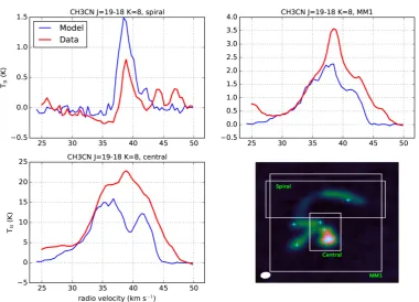
Figs11and12, respectively, show the spectra around the compact sources and on the same extended areas of interest as in the presen-tation of theK=4 model. The brightness match is reasonably good for all compact sources except for Main, and the line-width is only unmatched for MNE. The brighter observed line in Main suggests that the model should be warmer at radii<100 au. The broader observed line in MNE could be due to contamination from Main. We expect to obtain ALMA long-baseline data in the near future to disentangle this crowded region and produce a more detailed model of the Main-MNE system. The match to the extended areas (Fig.12) is within a factor of 2 in brightness for the large filament and the entire MM1, and better for the central region. In the latter, there is some missingemissionin the model at velocities close to the peak velocity of the entire MM1 core (≈38 km s−1_{). This peak is well} reproduced by theK=4 model (see Fig.9).

5 D I S C U S S I O N

5.1 An accretion filament feeding the fragmented high-mass core W33A MM1

One of the main results of this study is to show, via 3D radiative transfer modelling, that the elongated structure north of the MM1 core is an accretion (feeding) flow. The observed kinematics and modelling show that the filament has both longitudinal and radial motions, and that it is filled with high-density (≈8×107_cm−3_, see Table2), warm (∼200 K) gas. The velocity dispersion within this spiral-like filament could only be reproduced if an extra, radial velocity component was added (see Section 4.1.2). Given the high density and the existence of fragmentation within the filament – compact source Ridge –, infall is a plausible explanation to the observed extra velocity dispersion.

The total gas mass in the model ‘feeding’ filament is 0.41 M_⊙, and its average flow rate is 4.75×10−5_M

⊙yr−1. It is possible that

these are lower limits, since less dense, colder gas in the flow would not emit significantly in the CH3CN lines. For the modelled mass inflow rate, the depletion time of the filament gas is∼8.3×103 _yr, quite short compared with the few×105 _{yr expected for massive} star formation (Zinnecker & Yorke2007). At first sight, this suggests that the ‘feeding filament’ could be a transient structure, unless re-plenishment from larger scales occurs. Several studies have shown evidence for the continuity of molecular-gas flows from scales of

∼10 pc down to<0.05 pc (e.g. Galv´an-Madrid et al.2009; Schnei-der et al.2010; Liu et al.2012; Nakamura et al.2012; Peretto et al.

2013). For the case of W33A, Galv´an-Madrid et al. (2010) reported that MM1 appears to be connected to MM2 by an extension of gas

∼12 000 au long in the northeast-southwest direction, similar to the orientation of the spiral-like filament. This possible larger-scale extension of the filament, however, is not modelled in this paper since it does not emit significantly in the observed CH3CN tran-sitions. Further evidence for replenishment in W33A comes from the pc-scale filaments seen in NH3 emission, which converge in position–position–velocity space at the position of MM1 (Galv´an-Madrid et al.2010).

The rate at which the model spiral-like filament provides mass to MM1 is an order of magnitude below the combined protostellar accretion rate of the model compact sources∼4.6×10−4_M

⊙yr−1

(see Table1), and dominated by the accretion on to Main. We con-sider two possible interpretations for this: the mismatch between the protostellar and core accretion rates could mean that the former will be significantly lower within a few×104_{yr, after the gas} reser-voir in the modelled filaments is depleted. This is consistent with the onset of ionization in source Main, which hosts a tiny hyper-compact HIIregion with an estimated size<100 au (van der Tak & Menten2005). On the other hand, it is possible that gas accretion will continue for longer time-scales if there is the aforementioned replenishment from larger scales and/or our mass estimates for the intra-core filaments are lower limits because some gas does not emit in the modelled CH3CN lines.

Spiral-like structures like the filament feeding MM1 have been observed both at smaller and larger scales, from low-mass pro-toplanetary discs/envelopes (102_{au, P´erez et al.2016; Yen et al.}

2017), to luminous, cluster-forming clumps (105_{au, Wright et al.}

2014; Liu et al.2015). Such spiral structures feeding material to nascent stellar systems form as a natural consequence of gravi-tational fragmentation in (radiation) hydrodynamical simulations (e.g. Bate2011; Vorobyov, Zakhozhay & Dunham2013). Our ob-servations and analytical model look similar to the simulations of massive star formation presented by Krumholz, Klein & McKee (2007), who calculated specific predictions for images taken with ALMA in CH3CN transitions. The synthetic images from those simulations show spiral filaments with typical length scales of a few thousand au, feeding a central object that reaches a stellar mass of 8 M_⊙and a few lower mass companions. Their total gas mass within∼1000 au of the central core reaches about 5 M_⊙. These characteristics are similar to those of our analytical model, although in the Krumholz et al. (2007) simulations such structures arise in the context of a massive fragmenting disc, whereas our model is ad hoc.

5.2 Accretion filaments joining pairs of protostars

Figure 11. Same as Fig.7for CH3CN J=19−18,K=8.

Figure 12. Same as Fig.9for CH3CN J=19−18,K=8.

The accretion rate across the E→MNE filament is half of the feeding rate of the larger, spiral-like filament, suggesting that most of the gas processed by the latter ends up in the Main/MNE system. This finding is consistent with models of star (cluster) formation

that emphasize the need for replenishment of gas from cloud to clump to core to protostellar scales (e.g. Bonnell, Vine & Bate

2004; Smith, Longmore & Bonnell2009; Ballesteros-Paredes et al.