ESPRIT-like two-dimensional direction finding for mixed circular and strictly noncircular sources based on joint diagonalization

(1)

This is a repository copy of ESPRIT-like two-dimensional direction finding for mixed circular and strictly noncircular sources based on joint diagonalization.

White Rose Research Online URL for this paper: http://eprints.whiterose.ac.uk/120209/

Version: Accepted Version

Article:

Chen, H., Hou, C., Zhu, W.P. et al. (4 more authors) (2017) ESPRIT-like two-dimensional direction finding for mixed circular and strictly noncircular sources based on joint

diagonalization. Signal Processing, 141. pp. 48-56. ISSN 0165-1684 https://doi.org/10.1016/j.sigpro.2017.05.024

Reuse

Items deposited in White Rose Research Online are protected by copyright, with all rights reserved unless indicated otherwise. They may be downloaded and/or printed for private study, or other acts as permitted by national copyright laws. The publisher or other rights holders may allow further reproduction and re-use of the full text version. This is indicated by the licence information on the White Rose Research Online record for the item.

Takedown

If you consider content in White Rose Research Online to be in breach of UK law, please notify us by

(2)

ESPRIT-like Two-dimensional Direction Finding for

Mixed Circular and Strictly Noncircular Sources Based

on Joint Diagonalization

Hua Chena, Chunping Houa, Wei-Ping Zhub, Wei Liuc, Yang-Yang Dongd,

Qing Wanga

a

School of Electronic Informatin Engineering, Tianjin University, Tianjin 300072, P. R. China.

b

Department of Electrical and Computer Engineering, Concordia University, Montreal, QC H3G 1M8, Canada.

c

Department of Electronic and Electrical Engineering, University of Sheffield, Sheffield S1 3JD, UK.

d

Key Laboratory of Electronic Information Countermeasure and Simulation Technology, Ministry of Education, Xidian University, Xian 710071, Shanxi, P. R. China.

Abstract

In this paper, a two-dimensional (2-D) direction-of-arrival (DOA) estimation

method for a mixture of circular and strictly noncircular signals is

present-ed baspresent-ed on a uniform rectangular array (URA). We first formulate a new

2-D array model for such a mixture of signals, and then utilize the observed

data coupled with its conjugate counterparts to construct a new data

vec-tor and its associated covariance matrix for DOA estimation. By exploiting

the second-order non-circularity of incoming signals, a computationally

ef-fective ESPRIT-like method is adopted to estimate the 2-D DOAs of mixed

sources which are automatically paired by joint diagonalization of two

direc-∗_{Corresponding author}

Email addresses: [email protected](Hua Chen),[email protected]

(Wei-Ping Zhu ),[email protected](Wei Liu),[email protected]

(3)

tion matrices. One particular advantage of the proposed method is that it

can solve the angle ambiguity problem when multiple incoming signals have

the same angleθ orβ. Furthermore, the theoretical error performance of the

proposed method is analyzed and a closed-form expression for the

determin-istic Cramer-Rao bound (CRB) for the considered signal scenario is derived.

Simulation results are provided to verify the effectiveness of the proposed

method.

Keywords:

Two-dimensional (2-D), direction of arrival (DOA), noncircular signal,

uniform rectangular array (URA), joint diagonalization, angle ambiguity.

1. Introduction

Direction-of-arrival (DOA) plays a significant role in the area of array

sig-nal processing [1, 2]. Recently, the second-order non-circularity of incoming

signals has been exploited in both one dimensional (1-D ) [3–8] and

two-dimensional (2-D) or multi-two-dimensional [9–15] DOA estimation. However,

the algorithms developed thus far only consider strictly noncircular

incom-ing signals. In practice, a more realistic case is a mixture of circular (e.g.

quadrature phase shift keying, QPSK) and strictly non-circular (e.g. binary

phase shift keying, BPSK) signals.

There have been several approaches for joint estimation of circular and

strictly noncircular signals in 1-D direction finding. In [16], a new data vector

containing both the original data and the conjugate version was proposed to

form two estimators for strictly noncircular and circular signals,

(4)

DOAs of strictly noncircular and circular signals separately by exploiting the

circularity difference between the two classes of signals. However, all these

algorithms require the computationally expensive peak search of the MUSIC

pseudo spectrum. Recently, an ESPRIT-based parameter estimation

algo-rithm was developed in [18] for the above case, where a closed-form expression

related to strictly noncircular and circular signals was derived for efficient

1-D 1-DOA estimation. In addition, in [19], a sparse representation algorithm for

mixed signals was proposed, where overcomplete dictionaries were exploited

subject to sparsity constraints to jointly represent the covariance and

ellip-tic covariance matrices of the array output. For the 2-D case, to our best

knowledge, the only work on joint direction estimation of circular and

non-circular signals was reported in [20] where four 1-D peak searching estimators

were constructed using two parallel uniform linear arrays (ULAs) along with

a computationally expensive MUSIC method. Besides, the method in [20]

can not solve the angle ambiguity problem when multiple incoming signals

have the same angle θ or β, and the theoretical performance analysis is not mentioned in [20]. More recently, an ESPRIT based method was proposed

in [21] to estimate 2-D angle parameters for bistatic MIMO radar using a

joint diagonalization algorithm. However, no noncircularity information is

considered in the formulation. Yang [22] proposed an ESPRIT algorithm for

coexistence of noncircular and circular sources in bistatic MIMO radar, but

it can not solve the angle ambiguity problem when multiple incoming signals

have the same angle θ or β. In addition, it needs additional procedure to

pair the 2-D angle parameters.

(5)

in this paper a method to deal with the 2-D DOA estimation problem in

the presence of a mixture of circular and strictly noncircular signals. Our

method utilizes a uniform rectangular array (URA) and an ESPRIT-like 2-D

DOA estimation algorithm to exploit the non-circularity information of the

impinging signals. By building a general 2-D array model with mixed circular

and strictly noncircular signals, we first construct a new data vector and its

associated covariance matrix by exploiting the observed array data coupled

with its conjugate counterpart. Then, an efficient ESPRIT-like method is

developed to estimate the 2-D DOA of the mixed sources, where the angleθ

or β are paired automatically, and meanwhile the angle ambiguity problem

of angle θ or β is settled, by joint diagonalization of two direction matrices.

Finally, the theoretical error performance of the proposed method is analyzed

and a closed-form expression for the deterministic Cramer-Rao bound (CRB)

for the mixed signals scenario is derived.

Throughout the paper, the notations (·)∗_{, (}_·₎T_{, (}_·₎−1_{, (}_·₎+_{, and (}_·₎H

rep-resent conjugation, transpose, inverse, pseudo-inverse, and conjugate

trans-pose, respectively. E(·) is the expectation operation; diag(·) stands for

the diagonalization operation; Ip denotes the p-dimensional identity matrix;

blkdiag(Z1,Z2) represents a block diagonal matrix with diagonal entries Z1

and Z2; the p×p matrix Υp denotes an exchange matrix with ones on its

anti-diagonal and zeros elsewhere; ⊗ is the kronecker matrix product

opera-tion; arg(·) is the phase; Re(·) and Im(·) denote the real and imaginary part;

ei denotes theith column of the identity matrix; tr(·) denotes the trace of a

(6)

x y

z

k

b

k

q

( )

k

s t

N

M

x

d

y

d

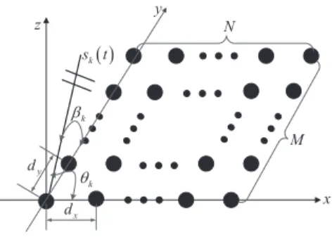
Fig. 1: Geometry of a URA

2. Array model

Consider K = Kn+Kc (assume the number of mixed signals is known)

uncorrelated far-field sources that are a mixture of Kn strictly noncircular

sources sn,k(t) and Kc circular sources sc,k(t) with identical wavelength λ.

They impinge on to an URA ofM×N omnidirectional sensors spaced bydx

in each row and dy in each column, as shown in Fig.1.

The direction of the kth signal is denoted as (θk, βk), k = 1,2, . . . , K.

Thus, the output of the array at time t can be modeled as

x(t) = As(t) +n(t) (1)

where x(t) = [x1(t),· · ·, xN(t), xN+1(t),· · · , x2N(t),· · · , xM N(t)]T is

com-posed of theM N received array signals,A= [a(θ1, β1),a(θ2, β2),· · · ,a(θK, βK)]T

is the array manifold matrix,s(t) = [s1(t), s2(t),· · · , sK(t)]T is the source

sig-nal vector andn(t) = [n1(t),· · · , nN(t), nN+1(t),· · ·, n2N(t),· · · , nM N(t)]T is

the additive white Gaussian complex circular noise vector with its elements

being of zero mean and variance σ2. The steering vector a(θk, βk) is given

by

(7)

where

ay(βk) = [1, ϕy(βk),· · ·ϕyM−1(βk)]T (3)

ax(θk) = [1, ϕx(θk),· · ·ϕxN−1(θk)]T (4)

with

ϕy(βk) = exp{j2πλ−1dycos (βk)} (5)

ϕx(θk) = exp{j2πλ−1dxcos (θk)} (6)

As in [18], we decompose each of the circular sources into two uncorrelated

strictly non-circular sources with the same DOA. Without loss of generality,

let the first Kn elements in s(t) represent the strictly non-circular signals.

Thus, s(t) can be represented as

s(t)=





Ψ 0 0

0 IKc jIKc



 

   

sn(t)

sr c(t)

sq c(t)



   

=Ψ1˜s(t) (7)

whereΨ=diag(ejφ1_{, . . . , e}jφKn) represents the rotation phases corresponding

to the strictly non-circular sources. Furthermore, Ψ1 is of sizeK ×K′ with

K′ ₌_K

n+ 2Kc and the real-valuedK′×1 vector ˜s(t) contains the symbols

of the Kn strictly non-circular sources sn(t) as well as theKc real partssrc(t)

andKc imaginary partssqc(t) of the circular signalssc(t). The array manifold

matrix A can be rewritten as

A = [An Ac] (8)

where An and Ac denote the array manifold matrix related to strictly

(8)

in (1) can be expressed as

x(t) =AΨ1˜s(t) +n(t) = ˜A˜s(t) +n(t) (9)

where ˜A=AΨ1 denotes the modified array manifold matrix.

For notional convenience, the indices of θ, β and t will be omitted in the

following discussion while not causing confusion.

3. The Proposed Method

In order to take advantage of the strict circularity of the strictly

non-circular sources and the virtual strict non-non-circularity of the non-circular sources,

a new data vector is defined by stacking the original data and its conjugate

counterpart as ˜ x=   x

ΥM Nx∗



=



 ˜ A˜s

ΥM NA˜

∗ ˜ s∗  +   n

ΥM Nn∗



 = ˘A˜s+ ˘n (10)

where ˘ A=   ˜ A

ΥM NA˜

∗   =  

AnΨ Ac

[

IKc jIKc

]

ΥM NA∗nΨ∗ ΥM NA∗c

[

IKc −jIKc

] 



(11)

is the extended array manifold matrix of size 2M N ×K′_,_n_˘ ₌



 n

ΥM Nn∗





is the 2M N ×1 noise vector, and ˜s = ˜s∗_{. Then, the covariance matrix of ˜}_x

is given by

R=E[˜xx˜H_{] = ˘}_AR

sA˘ H

+σ2I2M N (12)

(9)

Remark 1: In practice, only a finite number of observed data is available.

Thus, R has to be estimatedby

ˆ

R≈ 1

L

∑

l=1

ˆ˜

x(l)ˆ˜xH(l). (13)

where L denotes the number of snapshots.

Since the mixed signals are not correlated with each other, we perform

eigenvalue decomposition (EVD) of R as follows

R=UsΛsUHs +UnΛnUHn (14)

where the 2M N ×K′ _matrix _U

s and the 2M N ×(2M N −K′) matrix Un

are the signal subspace and noise subspace, respectively. TheK′×K′ matrix

Λs = diag(λ1,λ2· · ·,λK′) and the (2M N −K′)×(2M N −K′) matrix Λ_n=

diag(λK′₊₁,λ_K′₊₂· · ·,λ₂_{M N}) are corresponding diagonal matrices. λ₁ ≥λ₂ ≥

· · · ≥ λK′ > λ_K′₊₁ = · · · = λ₂_{M N} =σ2 are eigenvalues of R. As ˘A and U_s

span the same column space, there is a non-singular matrix T that satisfies

˘

A=UsT.

Define a new matrix Es as

Es=UsΛ

1 2

s, (15)

and four selection matrices as

J1a = [IN−1 0(N−1)×1] (16)

J1b = [0(N−1)×1 IN−1] (17)

J2a = [IM−1 0(M−1)×1] (18)

(10)

Then, the selection matrices of 1-D DOA θ of the mixed strictly

noncir-cular and cirnoncir-cular sources can be expressed as

J1 =blkdiag(J′1a,ΥM(N−1)J′1bΥM N) (20)

J2 =blkdiag(J′1b, ΥM(N−1)J′1aΥM N) (21)

where J′

1a=IM ⊗J1a and J′1b =IM ⊗J1b.

As for the selection matrices of 1-D DOA β, we have

J′₁ =blkdiag(J′2a,ΥN(M−1)J′2bΥM N) (22)

J′₂ =blkdiag(J′2b, ΥN(M−1)J′2aΥM N) (23)

where J′2a=J2a⊗IN and J′2b =J2b ⊗IN.

Next, we define two direction matrices related to θ and β as follows

Ωθ = (J1Es)+(J2Es) (24)

Ωβ = (J′1Es)+(J′2Es) (25)

It is noticed that in [22], the EVD of Ωθ and Ωβ is performed

indepen-dently as

Ωθ =UθΘθUHθ (26)

Ωβ =UβΘβUHβ (27)

where Uθ and Uβ are the K′ ×K′ unitary matrices, Θθ and Θβ are the

eigenvalue matrices that correspond to θ and β, respectively. It should be

pointed out that performing EVD of (26) and (27) separately, would lead to

the pairing problem between θ and β. Also, there are two identical

(11)

decomposed each circular source into two uncorrelated strictly non-circular

sources with the same DOA. This may cause rank-loss problem in (26) and

(27). Moreover, if the same θ orβ exists in the incoming mixed signals, the

eigenvalue spectrum in (26) and (27) may degenerate.

In order to solve the above three problems, we now apply the joint

diago-nalization method as used in blind signal separation [23] to the two direction

matrices Ωθ and Ωβ rather than perform EVD of Ωθ and Ωβ. Analogous to

[21], it can be easily deduced that

Ωθ = (J1Es)+(J2Es) = UΘθUH (28)

Ωβ = (J′1Es)+(J′2Es) = UΘβUH (29)

From (28) and (29), it can been seen that the requirement of joint

diag-onalization is satisfied according to Theorem 3 of [23]. By defining a set

Ω={Ωθ,Ωβ}, we know that there is a unitary matrix V that is essentially

equivalent to U, which minimizes the following nonnegative function

f(Ω,V) = ∑

i=θ,β

off(VHΩiV) (30)

where off(Mn×n) =

∑

1≤i̸=j≤n

|Mij|2, and matrix U is called a joint

diagonal-izer [23]. Since U is the eigenvector of both Ωθ and Ωβ, there is no need

for pairing betweenθ andβ since the one-to-one correspondence is preserved

on the diagonals between eigenvalue matrices Θθ and Θβ. The same joint

diagonalization procedure can be implemented by a series of Givens rotations

in [23, 24] to obtain the unitary matrixU. The key idea of joint

(12)

Jacobi-like algorithm with plane rotations, and the detailed pseudo code of

joint diagonalization procedure can be seen in [24].

Then we have eigenvalues of Ωθ and Ωβ computed as

ηθk =u H

kΩθuk (31)

ηβk =u H

kΩβuk (32)

whereuk (k= 1, . . . , K′) is thekth column ofU. From (31) and (32), it can

be easily obtained that

θk = arccos

(_λ_arg(_η

θk) 2πdx

)

(33)

βk= arccos

(_λ_arg(_η

βk) 2πdy

)

(34)

It should be noted that due to the decomposition of each circular source

into two strictly non-circular sources, we have obtained K′ _{angle estimates}

for either θk or βk, while only K actual 2-D DOAs are present. Thus, we

need to correctly pair the two estimates obtained for each circular source in

a suitable manner. Actually, this can be easily done by finding the same

estimates for each θk orβk and then calculating the average of two identical

estimates for 2-D DOA θc,k and βc,k(k = 1, . . . , Kc) respectively as

θc,k= (θ1

c,k+θ2c,k)

2 (35)

βc,k = (β1

c,k+β2c,k)

2 (36)

Clearly, due to the automatically paired relationship between θk and βk,

all the circular sources have been separated provided that either θk or βk

(13)

Table 1: Summary of the proposed method.

Input: {xˆ˜(l)}L

l=1: L snapshots of the new constructed array output vector.

Output: ˆθk and ˆβk: pair-free 2-D estimated angles of K mixed signals.

Step 1 Estimate the covariance matrix ˆR≈ _L1

L

∑

l=1

ˆ˜

x(l)ˆ˜xH_(l).

Step 2 Perform subspace decomposition ˆR= ˆUsΛˆsUˆ

H

s + ˆUnΛˆnUˆ H n to

get Ûs, and then compute Ês= ÛsΛˆ

1 2

s.

Step 3 Construct two direction matrices ˆΩθ = (J1Eˆs)+(J2Eˆs) and

ˆ

Ωβ = (J′₁Eˆs)+(J′₂Eˆs).

Step 4 Implement the joint diagonalization to the set ˆΩ={Ωˆθ,Ωˆβ} to

obtain the unitary matrix ˆU by a series of Givens rotations.

Step 5 Compute the eigenvalues ˆηθk = ˆu

H

kΩˆθuˆk and ˆηβk = ˆu H kΩˆβuˆk

Step 6 Compute the 2-D DOAs as ˆθk= arccos

(_λ_arg(ˆ_η

θk) 2πdx

) and ˆ

βk= arccos

(_λ_arg(ˆ_η

βk) 2πdy

)

(k = 1, . . . , K′₎

Step 7 Compute the 2-D DOAs of circular signals as ˆθc,k =

(ˆθ1

c,k+ˆθ2c,k) 2

and ˆβc,k = ( ˆβ1

c,k+ ˆβ2c,k)

(14)

estimation under the mixed circular and strictly noncircular sources is

sum-marized in Table 1.

Remark 2: Since the noncircularity information is used in the proposed

method, the equivalent number of degrees of freedom of the array is increased

compared to the method in [21]. The maximum number of identifiable targets

by the proposed method isKn+2Kc =min{2M(N −1),2N(M −1)}, while

that of the method in [21] must satisfyKn+Kc =min{M(N −1), N(M −1)}.

Therefore, our method can distinguish more signals than the method in [21],

when at least two strictly non-circular sources are present in the mixed

sig-nals.

Remark 3: The major part of the computational effort of the proposed

method includes the construction of ˆR, performing EVD of ˆR, and joint

diagonalization of the setΩ. To calculate ˆR, we needO((2M N)2L)complex

multiplications; the EVD operation of ˆR requires the amount of complex

multiplications of O((2M N)3)

; and jointly diagonalizing the set Ω (two

K′_×_K′ _{direction matrices), is of}_O(

2(K′₎3)

. Then, the total computational

complexity of the proposed method in terms of complex multiplications is

about O(

(2M N)2L+ (2M N)3+ 2(K′₎3)

.

Remark 4: The proposed method is also applicable to the case where

all the incoming signals are noncircular signals (Case 4) since the uniqueness

of joint diagonalization is still satisfied for this case. The simulation results

in section IV will demonstrate the correctness of Case 4. And the 2-D angle

(15)

4. Theoretical error performance analysis

In this section, the theoretical error performance analysis of the proposed

method is conducted. The derivation in this paper is along the lines of

the first-order analysis done by Rao [25] and the backward error analysis

by Li [26]. To analyze the proposed subspace algorithm, it is important to

analyze the subspace perturbation. First, subspace decomposition can also

be performed using singular value decomposition (SVD) of ˜x as follows:

˜

x=( _U_s _U_n )





Σs 0

0 0



 



VH

s

VHn



 (37)

Following the first-order approximation principles [25, 26] for eigenvalues

in (31) and (32), we have

δηθk ≈u H

kδΩθuk =uHk(J1Ux)+(δUx2−δUx1Ωθ)uk (38)

δηβk ≈u H

kδΩβuk=uHk(J

′

1Ux)+(δUx2 −δUx1Ωβ)uk (39)

where

Ux =UsΣs (40)

δUx =δUsΣs (41)

δUs =UnUHnnV˘ sΣ−

1

s (42)

According to (41) and (42), we obtain

δUx1 =J1δUx = (J1Un)UHnnV˘ s (43)

δUx2 =J2δUx = (J2Un)UHnnV˘ s (44)

δU′x1 =J

′

(16)

δU′

x2 =J′2δUx = (J′2Un)UHnnV˘ s (46)

Then, by substituting (43) and (44) into (38), (45) and (46) into (39),

(38) and (39) can be rewritten as

δηθk ≈u H

k(J1Ux)+(J2Un−ηθkJ1Un)U H

nnV˘ suk (47)

δηβk ≈u H k(J

′

1Ux)+(J′₂Un−ηβkJ

′

1Un)UHnnV˘ suk (48)

Using the first-order Taylor series expansion [25, 26], the perturbation of

the kth (k= 1, . . . , K′₎ _θ _and _β _{can be expressed as}

δθk =νθkIm

( δηθk

ηθk

)

(49)

δβk=νβkIm

( δηβk

ηβk

)

(50)

where νθk=λ/(2πdxsinθk) and νβk=λ/(2πdysinβk). The error-variance of

the estimated 2-D DOAs are

var (δθk) =

1 2ν

2 θkvar

(

ξH_θ

knϑ˘ k

ηθk

)

= ν

2 θkσ

2

ξ_θH

kξθkϑ H kϑk |ηθk|

2 (51)

var (δβk) =

1 2ν

2 βkvar

(

ξH_β

knϑ˘ k

ηβk

)

= ν

2 βkσ

2

ξH_β

kξβkϑ H kϑk |ηβk|

2 (52)

where

ξ_θH

k =u H

k(J1Ux)+(J2Un−ηθkJ1Un)U H

n (53)

ξ_βH

k =u H k(J

′

1Ux)+(J′₂Un−ηβkJ

′

1Un)UHn (54)

ϑk =Vsuk (55)

(17)

For the kth (k = 1, . . . , Kc) circular signals, the variances of the two

estimated angles are given by

var (δθc,k) =

[

var(

δθc,k1

)

+ var(

δθc,k2

)]/

2 (57)

var (δβc,k) =

[

var(

δβ_c,k1 )+ var(

δβ_c,k2 )]/2 (58)

5. Cramer-Rao bound (CRB) analysis

In this section, we derive the closed-form expression of the deterministic

CRB of 2-D DOAs for the mixed signals scenario. With (8), the model in

(1) can be rewritten as

x=AnΨsn+Acsc +n (59)

The desired CRB matrix is usually computed by taking the inverse of the

Fisher information matrix (FIM)Ffor the interest parameterθ = [θn,1, θn,2, . . . ,

θn,Kn, θc,1, θc,2, . . . , θc,Kc] and β = [βn,1, βn,2, . . . , βn,Kn, βc,1, βc,2, . . . , βc,Kc]. F

can be written as

F=



      

Fθnθn Fθnθc Fθnβn Fθnβc

Fθcθn Fθcθc Fθcβn Fθcβc

Fβnθn Fβnθc Fβnβn Fβnβc

Fβcθn Fβcθc Fβcβn Fβcβc



      

(60)

Note that the (i, j)th element of Fθnθn [27, 28] is given by

F(θn,i, θn,j) = 2 Re{tr[( ˙Aθn,iΨsn)

H_γ−1_{( ˙}_A

θn,jΨsn)]}

= 2 Re{tr[( ˙AθnΨeie T

i sn)Hγ−1( ˙AθnΨeje T jsn)]}

= 2 Re[(eT

i Ψ H_A_˙H

θnγ

−1_A_˙

θnΨej)(e T

jsnsHnei)]

= 2LRe[(ΨH_A_˙H

θnγ

−1_A_˙

θnΨ)ij(R T snsn)ij]

(18)

Due toF=FT_{, we only need to calculate the upper triangular block matrices}

of F. Similarly, we get the (i, j)th element of block matrix Fθnθc, Fθnβn,

Fθnβc,Fθcθc, Fθcβn, Fθcβc, Fβnβn,Fβnβc and Fβcβc respectively, as follows

F(θn,i, θc,j) = 2 Re{tr[( ˙Aθn,iΨsn)

H_γ−1_{( ˙}_A

θc,jsc)]}

i sn)Hγ−1( ˙Aθceje T jsc)]}

= 2 Re[(eT

i Ψ H_A_˙H

θnγ

−1_A_˙

θcej)(e T

jscsHnei)]

= 2LRe[(ΨH_A_˙H

θnγ

−1_A_˙

θc)ij(R T scsn)ij]

(62)

F(θn,i, βn,j) = 2 Re{tr[( ˙Aθn,iΨsn) H

γ−1( ˙Aβn,jΨsn)]}

isn)Hγ−1( ˙AβnΨeje T jsn)]}

= 2 Re[(eTi Ψ H _˙

AHθnγ

−1_A_˙

βnΨej)(e T

jsnsHnei)]

= 2LRe[(ΨHA˙Hθnγ

−1_A_˙

βnΨ)ij(R T snsn)ij]

(63)

F(θn,i, βc,j) = 2 Re{tr[( ˙Aθn,iΨsn)

H_γ−1_{( ˙}_A

βc,jsc)]}

i sn)Hγ−1( ˙Aβceje T jsc)]}

= 2 Re[(eT

i ΨHA˙ H θnγ

−1_A_˙

βcej)(e T

jscsHnei)]

= 2LRe[(ΨH_A˙ H

θnγ

−1_A_˙

βc)ij(R T scsn)ij]

(64)

F(θc,i, θc,j) = 2 Re{tr[( ˙Aθc,isc)

H_γ−1_{( ˙}_A

θc,jsc)]}

= 2 Re{tr[( ˙Aθceie T

i sc)Hγ−1( ˙Aθceje T jsc)]}

= 2 Re[(eT

i A˙ H θcγ

−1_A_˙

θcej)(e T

jscsHc ei)]

= 2LRe[( ˙AH_θ_cγ−1A˙θc)ij(R T scsc)ij]

(19)

F(θc,i, βn,j) = 2 Re{tr[( ˙Aθc,isc)

H_γ−1_{( ˙}_A

βn,jΨsn)]}

i sc)Hγ−1( ˙AβnΨeje T jsn)]}

= 2 Re[(eT

i A˙ H θcγ

−1_A_˙

βnΨej)(e T

jsnsHc ei)]

= 2LRe[( ˙AH_θ_cγ−1A˙βnΨ)ij(R T snsc)ij]

(66)

F(θc,i, βc,j) = 2 Re{tr[( ˙Aθc,isc)

H_γ−1_{( ˙}_A

βc,jsc)]}

i sc)Hγ−1( ˙Aβceje T jsc)]}

= 2 Re[(eTi A˙ H θcγ

−1_A_˙

βcej)(e T

jscsHc ei)]

= 2LRe[( ˙AHθcγ

−1_A_˙

βc)ij(R T scsc)ij]

(67)

F(βn,i, βn,j) = 2 Re{tr[( ˙Aβn,iΨsn) H

γ−1( ˙Aβn,jΨsn)]}

= 2 Re{tr[( ˙AβnΨeie T

i sn)Hγ−1( ˙AβnΨeje T jsn)]}

= 2 Re[(eTi Ψ H _˙

AHβnγ

−1_A_˙

βnΨej)(e T

jsnsHnei)]

= 2LRe[(ΨHA˙Hβnγ

−1_A_˙

βnΨ)ij(R T snsn)ij]

(68)

F(βn,i, βc,j) = 2 Re{tr[( ˙Aβn,iΨsn)

H_γ−1_{( ˙}_A

βc,jsc)]}

= 2 Re{tr[( ˙AβnΨeie T

i sn)Hγ−1( ˙Aβceje T jsc)]}

= 2 Re[(eT

i ΨHA˙ H βnγ

−1_A_˙

βcej)(e T

jscsHnei)]

= 2LRe[(ΨHA˙Hβnγ

−1_A_˙

βc)ij(R T scsn)ij]

(69)

F(βc,i, βc,j) = 2 Re{tr[( ˙Aβc,isc)

H_γ−1_{( ˙}_A

βc,jsc)]}

= 2 Re{tr[( ˙Aβceie T

i sc)Hγ−1( ˙Aβceje T jsc)]}

= 2 Re[(eT

i A˙ H βcγ

−1_A_˙

βcej)(e T

jscsHc ei)]

= 2LRe[( ˙AHβcγ

−1_A_˙

βc)ij(R T scsc)ij]

(20)

where ˙Aςn, ˙Aςc (ς =θ, β), Rsnsn, Rsnsc, Rscsn and Rscsc has the form of

˙

Aςn=

[ ∂A ∂ς1

,∂A ∂ς2

,..., ∂A ∂ςKn

]

(71)

˙ Aςc=

[ ∂A ∂ς1

,∂A ∂ς2

,..., ∂A ∂ςKc

]

(72)

Rsnsn =

1 Lsns

H

n (73)

Rsnsc =

1 Lsns

H

c (74)

Rscsn =

1 Lscs

H

n (75)

Rscsc =

1 Lscs

H

c (76)

for white noise, γ has the form of σ2IM N.

According to equations from (71) to (76), we obtain

Fθnθn = 2LRe[(ΨHA˙

H θnγ

−1_A_˙

θnΨ)⊗(R T

snsn)] (77)

Fθnθc = 2LRe[(ΨHA˙

H θnγ

−1_A_˙

θc)⊗(R T

scsn)] (78)

Fθnβn = 2LRe[(ΨHA˙

H θnγ

−1_A_˙

βnΨ)⊗(R T

snsn)] (79)

Fθnβc = 2LRe[(ΨHA˙

H θnγ

−1_A_˙

βc)⊗(R T

scsn)] (80)

Fθcθc = 2LRe[( ˙A

H θcγ

−1_A_˙

θc)⊗(R T

scsc)] (81)

Fθcβn = 2LRe[( ˙A

H θcγ

−1_A_˙

βnΨ)⊗(R T

snsc)] (82)

Fθcβc = 2LRe[( ˙A

H θcγ

−1_A_˙

βc)⊗(R T

scsc)] (83)

Fβnβn = 2LRe[(ΨHA˙

H βnγ

−1_A_˙

βnΨ)⊗(R T

snsn)] (84)

Fβnβc = 2LRe[(ΨHA˙

H βnγ

−1_A_˙

βc)⊗(R T

scsn)] (85)

Fβcβc = 2LRe[( ˙A

H βcγ

−1_A_˙

βc)⊗(R T

(21)

Then the CRB matrix Ccan be expressed as

C=F−1 ₍₈₇₎

and the individual CRBs of θ and β for the circular signals as well as the

strictly non-circular signals can easily be extracted from (87) as follows

CRBθi =Ci,i (88)

CRBβi =Ci+K,i+K (89)

where Ci,i (i= 1,2, . . . , K) denotes the (i, i)th element of C.

It should be pointed out that the above CRB analysis is also applicable

to the case where all the incoming signals are noncircular or circular signals.

6. Simulation results

In this section, five sets of simulations are performed to demonstrate the

performance of the proposed method. The first set of simulation is based

on a URA with M = 3 rows and N = 4 columns, while for the next three,

N = M = 5; and for the last one, the number of antennas varies. Both dx

and dy are half wavelength.

The mixed circular and strictly noncircular signals have an equal power.

The power of additive white Gaussian noise is σ2n. The signal-to-noise ratio

is defined as SNR = 10log₁₀(σ2

s/σn2). The root mean squared error (RMSE)

as defined by RMSE = √

1 KMc

K

∑

k=1 Mc

∑

q=1

(ˆζqk−ζk) 2

is adopted for quantitative

evaluation, where Mc is the number of Monte Carlo simulations, K is the

number of signals, ζˆq,k is the estimate of the parameter (ˆθk or ˆβk) in the kth

(22)

βk. For comparison, the DOA estimation results obtained using the method

in [21], which does not exploit the noncircular information of the signals,

the theoretical error performance and CRB of the proposed method are also

provided. Note that we cannot compare with the method in [22], because

when the angle ambiguity problem emerges, the method in [22] fails to work.

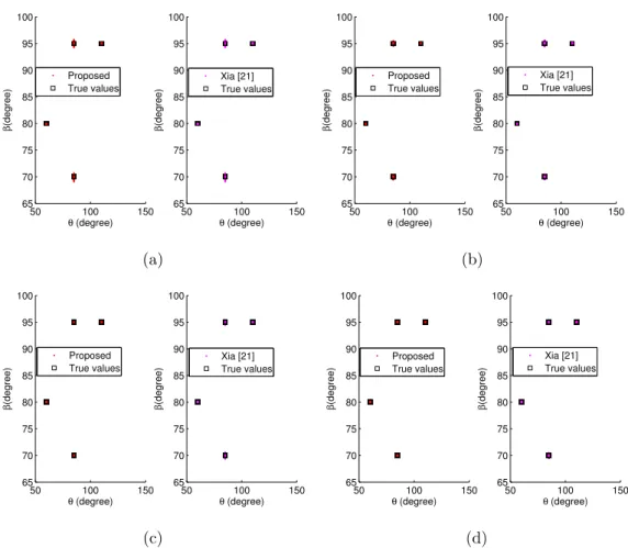
6.1. 2-D DOA estimation

We consider four uncorrelated mixed BPSK and QPSK signals from

di-rections (60◦_,₈₀◦_{), (85}◦_,₇₀◦_{), (85}◦_,₉₅◦_{) and (110}◦_,₉₅◦_{), respectively. Four}

cases are studied corresponding to one, two and four BPSK signals. The

SNR is set at 10dB. The number of snapshots is 500, and Mc is 500. Fig.2

(a) to (d) displays the 2-D DOA scattergram of the circular and strictly

non-circular signals by both the proposed method and the method in [21], with

number of strictly noncircular signals increasing from one to four. It can be

seen that the proposed method outperforms the method in [21], especially

when the number of strictly noncircular signals increases. This is because the

noncircularity information is utilized in the proposed method which increases

the effective array aperture.

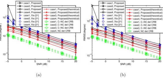
6.2. Performance versus SNR

In this simulation, we study the performance with respect to a varying

S-NR ranging from -5dB to 20dB. Here we suppose four uncorrelated mixed

sig-nals are from directions (60◦_,₅₀◦_{), (70}◦_,₅₀◦_{), (70}◦_,₆₀◦_{) and (80}◦_,₇₀◦_{). Three}

cases are considered as before starting fromKn = 1 associated with (60◦,50◦)

up to Kn = 4 with all above signals. The number of snapshots is 800 and

(23)

50 100 150 65 70 75 80 85 90 95 100

θ (degree)

β

(degree)

50 100 150

65 70 75 80 85 90 95 100

θ (degree)

β (degree) Proposed True values Xia [21] True values (a)

50 100 150

65 70 75 80 85 90 95 100

θ (degree)

β

(degree)

50 100 150

65 70 75 80 85 90 95 100

θ (degree)

β (degree) Proposed True values Xia [21] True values (b)

50 100 150

65 70 75 80 85 90 95 100

θ (degree)

β

(degree)

50 100 150

65 70 75 80 85 90 95 100

θ (degree)

β (degree) Proposed True values Xia [21] True values (c)

50 100 150

65 70 75 80 85 90 95 100

θ (degree)

β

(degree)

50 100 150

65 70 75 80 85 90 95 100

θ (degree)

β (degree) Proposed True values Xia [21] True values (d)

Fig. 2: 2-D scattergram for mixed signals. (a) Case 1: one BPSK and three QPSK signals.

(b) Case 2: two BPSK and two QPSK signals. (c) Case 3: three BPSK and one QPSK

(24)

−5 0 5 10 15 20 10−2

10−1 100

SNR (dB)

RMSE(degree )

case1, Proposed case2, Proposed case3, Proposed case4, Proposed case1, Xia [21] case2, Xia [21] case3, Xia [21] case4, Xia [21]

case1, Proposed(theoretical) case2, Proposed(theoretical) case3, Proposed(theoretical) case4, Proposed(theoretical) case1, C−NC det CRB case2, C−NC det CRB case3, C−NC det CRB case4, NC det CRB

(a)

−5 0 5 10 15 20 10−2

10−1 100

SNR (dB)

RMSE(degree)

(b)

Fig. 3: RMSE of versus SNR with the number of snapshots to be 800. (a)θ. (b)β.

the proposed method for both angles are superior to that of the method in

[21] in all four cases. As before, the performance of the proposed method

im-proves consistently from case 1 to case 4, with more and more noncircularity

information available.

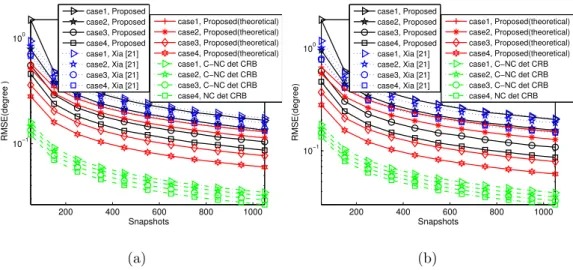
6.3. Performance versus snapshots

The performance of the proposed method is studied in this part with the

number of snapshots varying from 50 to 1050. The SNR is fixed at 5 dB

and the other parameters are the same as in Sec.6.2. Simulation results are

shown in Fig.4 (a) and (b), and we can draw similar conclusions as in Sec.6.2.

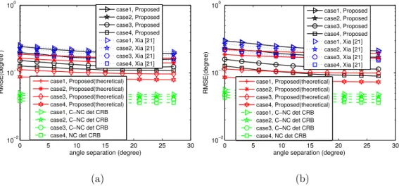
6.4. Performance versus angle separation

Now the performance of the proposed method is investigated with the

angle separation ∆ of 2-D DOAs varying from 0 to 27. The SNR is fixed at

5dB and the snapshot number is 500. Four uncorrelated signals arrive from

(25)

200 400 600 800 1000 10−1

100

Snapshots

RMSE(degree )

(a)

200 400 600 800 1000 10−1

100

Snapshots

RMSE(degree)

(b)

Fig. 4: RMSE of versus snapshots with SNR fixed at 5dB. (a)θ. (b)β.

and ((80 + ∆)◦_,_{(70 + ∆)}◦_{). We also consider four cases where one, two, three}

and four BPSK signals are present. Naturally, as angle separation varies

from small to large, all methods perform well since the joint diagonalization

procedure can solve the angle ambiguity problem, as shown in Fig.5 (a) and

(b). Moreover, our proposed method again outperforms the method in [21]

for all four cases.

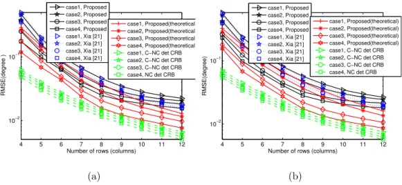
6.5. Performance versus number of rows (columns)

Now we study the effect of array size on the performance. M and N are

assigned the same value and vary from 4 to 12. The SNR is fixed at 5dB

and the number of snapshot is 800. Fig.6 (a) and (b) show the RMSE of

estimated angles obtained by the algorithm in [21] and the proposed one.

From case 1 to case 4, it can be seen that the superiority of our proposed

algorithm is more significant when the size of array is small such as when

the number of rows (columns) equals 4 or 5. When the size of array becomes

(26)

0 5 10 15 20 25 30 10−2

10−1 100

angle separation (degree)

RMSE(degree )

(a)

0 5 10 15 20 25 30

10−2 10−1 100

angle separation (degree)

RMSE(degree)

(b)

Fig. 5: RMSE of versus angle separation with SNR fixed at 5dB and the snapshot number

to be 500. (a)θ. (b)β.

[21]. This is because when the number of rows (columns) is increased, the size

of the new data vector ˜xbecomes larger, and the accuracy of the estimated

covariance matrix of ˜xwill be worse with given the number of snapshots. We

can improve this phenomenon by increasing the number of snapshots.

7. Conclusion

A 2-D DOA estimation method using the URA has been proposed for a

mixture of circular and strictly noncircular signals. Based on an

ESPRIT-like method, the estimated 2-D DOAs of the sources are paired automatically

by joint diagonalization of two direction matrices. The theoretical error

per-formance of the proposed method is analyzed and a closed-form expression

for the deterministic CRB of 2-D DOAs for the mixed signals scenario is

de-rived. Simulation results show that the performance of the proposed method

(27)

non-4 5 6 7 8 9 10 11 12 10−2

10−1

Number of rows (columns)

RMSE(degree )

(a)

4 5 6 7 8 9 10 11 12 10−2

10−1

Number of rows (columns)

RMSE(degree)

(b)

Fig. 6: RMSE of versus number of rows (columns) with SNR fixed at 5dB and the snapshot

number to be 800. (a) θ. (b)β.

circularity information of the impinging signals.

Acknowledgement

This work is supported by the National 863 Programs under Grant (No.

2015AA01A706) and China Scholarship Council (CSC).

[1] H. Krim, M. Viberg,“Two Decades of Array Signal Processing

Research-The Parametric Approach,” IEEE Signal Processing Magazine, vol. 13,

no. 4, pp. 67–94, 1996.

[2] A.B. Gershman, M. Rbsamen, M. Pesavento, “One-and two-dimensional

direction-of-arrival estimation: An overview of search-free techniques,”

Signal Processing, vol. 90, no. 5, pp. 1338–1349, 2010.

(28)

ar-rival for noncircular sources,” IEEE Transactions on Signal Processing,

vol. 54, no. 7, pp. 2678–2690, 2006.

[4] J. Liu, Z. Huang and Y. Zhou, “Extended 2q-MUSIC algorithm for

noncircular signals,” Signal Processing, vol. 88, no. 6, pp. 1327–1339,

2008.

[5] H. Abeida and J.-P. Delmas, “Statistical performance of MUSIC-like

al-gorithms in resolving noncircular sources,”IEEE Transactions on Signal

Processing, vol. 56, no. 9, pp. 4317–4329, 2008.

[6] S. B. Hassen, F. Belliliand, A. Samet and S. Affes, “DOA Estimation of

Temporally and Spatially Correlated Narrowband Noncircular Sources

in Spatially Correlated White Noise,”IEEE Transactions on Signal

Pro-cessing, vol. 59, no. 9, pp. 4108–4121, 2011.

[7] Y. Shi, X. Mao, M. Cao, and Y. Liu, “Deterministic maximum

likeli-hood method for direction-of-arrival estimation of strictly noncircular

signals,” in Acoustics, Speech and Signal Processing (ICASSP), 2016

IEEE International Conference on. IEEE, 2016, pp. 3061–3065.

[8] S. Cao, D. Xu, X. Xu and Z. Ye, “DOA estimation for noncircular

signals in the presence of mutual coupling,” Signal Processing, vol. 105,

pp. 12–16, 2014.

[9] J. Liu, Z. Huang, and Y. Zhou, “Azimuth and elevation estimation for

noncircular signals,” Electronics letters, vol. 43, no. 20, pp. 1117–1119,

(29)

[10] L. Gan, J.-F. Gu, and P. Wei, “Estimation of 2-D DOA for noncircular

sources using simultaneous svd technique,” IEEE Antennas and

Wire-less Propagation Letters, vol. 7, pp. 385–388, 2008.

[11] F. Roemer, and M. Haardt, “Multidimensional unitary Tensor-ESPRIT

for Non-Circular sources,” in Acoustics, Speech and Signal Processing

(ICASSP), 2009 IEEE International Conference on. IEEE, 2009, pp.

3577–3580.

[12] J. Steinwandt, F. Roemer, and M. Haardt, “Analytical performance

evaluation of multi-dimensional Tensor-ESPRIT-based algorithms for

strictly non-circular sources,” in Sensor Array and Multichannel Signal

Processing Workshop (SAM), 2016 IEEE International Conference on.

IEEE, 2016.

[13] Y. Shi, L. Huang, C. Qian, and H.C. So, “Direction-of-arrival

estima-tion for noncircular sources via structured least squares-based esprit

using three-axis crossed array,” IEEE Transactions on Aerospace and

Electronic, vol. 51, no. 2, pp. 1267–1278, 2015.

[14] J. Steinwandt, F. Roemer, M. Haardt, and G. Del Galdo,

“R-dimensional ESPRIT-type algorithms for strictly second-order

non-circular sources and their performance analysis,” IEEE Transactions

on Signal Processing, vol. 62, no. 18, pp. 4824–4838, 2014.

[15] J. Steinwandt, F. Roemer, M. Haardt, and G. Del Galdo, “Deterministic

(30)

anal-ysis of the achievable gains,” IEEE Transactions on Signal Processing,

vol. 64, no. 17, pp. 4417–4431, 2016.

[16] F. Gao, A. Nallanathan, and Y. Wang, “Improved music under the

co-existence of both circular and noncircular sources,” IEEE Transactions

on Signal Processing, vol. 56, no. 7, pp. 3033–3038, 2008.

[17] A. Liu, G. Liao, Q. Xu, and C. Zeng, “A circularity-based doa estimation

method under coexistence of noncircular and circular signals,” in

Acous-tics, Speech and Signal Processing (ICASSP), 2012 IEEE International

Conference on. IEEE, 2012, pp. 2561–2564.

[18] J. Steinwandt, F. Roemer, and M. Haardt, “ Esprit-type algorithms for a

received mixture of circular and strictly non-circular signals, ” in

Acous-tics, Speech and Signal Processing (ICASSP), 2015 IEEE International

Conference on. IEEE, 2015, pp. 2809-2813.

[19] Z.-M. Liu, Z.-T. Huang, Y.-Y. Zhou, and J. Liu, “Direction-of-arrival

es-timation of noncircular signals via sparse representation,” IEEE

Trans-actions on Aerospace and Electronic Systems, vol. 48, no. 3, pp. 2690–

2698, 2012.

[20] H. Chen, C.-P. Hou, W. Liu, W.-P. Zhu and M.N.S. Swamy, “Efficient

Two-Dimensional Direction of Arrival Estimation for a Mixture of

Cir-cular and NoncirCir-cular Sources,” IEEE Sensors Journal, vol. 16, no. 8,

pp. 2527–2536, 2016.

[21] T.Q. Xia, “ Joint diagonalization based DOD and DOA estimation for

(31)

[22] X. Yang, G. Zheng and J. Tang, “ESPRIT algorithm for coexistence of

circular and noncircular signals in bistatic MIMO radar” inIEEE Radar

Conference (RadarConf ), IEEE, 2016, pp. 1-4.

[23] A. Belouchrani, K. Abed-Meraim, J.F. Cardoso, and E. Moulines, “ A

blind source separation technique using second-order statistics” IEEE

Transactions on Signal Processing, vol. 45, no. 2, pp. 434–444, 1997.

[24] Y. Y. Dong, C. X. Dong, Y. T. Zhu, G. Q. Zhao,and S. Y. Liu, “

Two-dimensional DOA estimation for L-shaped array with nested subarrays without pair matching” IET Signal Processing, vol. 10, no. 9, pp. 1112–

1117, 2016.

[25] B. D. Rao and K. V. S. Hari, “Performance analysis of ESPRIT and

TAM in determining the direction of arrival of plane waves in noise,”

IEEE Transactions on acoustics, speech, and signal processing, vol. 37,

no. 12, pp. 1990–1995, 1989.

[26] F. Li, R. J. Vaccaro, and D. W. Tufts, “ Performance analysis of the

state-space realization (TAM) and ESPRIT algorithms for DOA

esti-mation,” IEEE Transactions on Antennas Propagation, vol. 39, no. 3,

pp. 418–423, 1991.

[27] M. Jin, G. Liao and J. Li, “ Joint DOD and DOA estimation for bistatic

MIMO radar,” Signal Processing, vol. 89, no. 2, pp. 244–251, 2009.

[28] Stoica P., Moses R.L., Spectral Analysis of Signals. Prentice-Hall, NJ,