https://doi.org/10.5194/acp-18-8647-2018 © Author(s) 2018. This work is distributed under the Creative Commons Attribution 4.0 License.
On the discrepancy of HCl processing in the core of the wintertime
polar vortices
Jens-Uwe Grooß1, Rolf Müller1, Reinhold Spang1, Ines Tritscher1, Tobias Wegner1,a, Martyn P. Chipperfield2, Wuhu Feng2,3, Douglas E. Kinnison4, and Sasha Madronich4
1Institut für Energie- und Klimaforschung – Stratosphäre (IEK-7), Forschungszentrum Jülich, Jülich, Germany 2School of Earth and Environment, University of Leeds, Leeds, UK
3National Centre for Atmospheric Science, University of Leeds, Leeds, UK
4Atmospheric Chemistry Observations and Modeling Laboratory, National Center for Atmospheric Research,
Boulder, CO, USA
anow at: KfW Bankengruppe, Frankfurt, Germany
Correspondence:Jens-Uwe Grooß ([email protected]) Received: 23 February 2018 – Discussion started: 28 February 2018 Revised: 24 May 2018 – Accepted: 29 May 2018 – Published: 20 June 2018
Abstract. More than 3 decades after the discovery of the ozone hole, the processes involved in its formation are be-lieved to be understood in great detail. Current state-of-the-art models can reproduce the observed chemical com-position in the springtime polar stratosphere, especially re-garding the quantification of halogen-catalysed ozone loss. However, we report here on a discrepancy between simula-tions and observasimula-tions during the less-well-studied period of the onset of chlorine activation. During this period, which in the Antarctic is between May and July, model simula-tions significantly overestimate HCl, one of the key chemi-cal species, inside the polar vortex during polar night. This HCl discrepancy is also observed in the Arctic. The dis-crepancy exists in different models to varying extents; here, we discuss three independent ones, the Chemical Lagrangian Model of the Stratosphere (CLaMS) as well as the Eulerian models SD-WACCM (the specified dynamics version of the Whole Atmosphere Community Climate Model) and TOM-CAT/SLIMCAT. The HCl discrepancy points to some un-known process in the formulation of stratospheric chemistry that is currently not represented in the models.
We characterise the HCl discrepancy in space and time for the Lagrangian chemistry–transport model CLaMS, in which HCl in the polar vortex core stays about constant from June to August in the Antarctic, while the observations indicate a continuous HCl decrease over this period. The somewhat smaller discrepancies in the Eulerian models SD-WACCM
and TOMCAT/SLIMCAT are also presented. Numerical dif-fusion in the transport scheme of the Eulerian models is iden-tified to be a likely cause for the inter-model differences. Al-though the missing process has not yet been identified, we investigate different hypotheses on the basis of the charac-teristics of the discrepancy. An underestimated HCl uptake into the polar stratospheric cloud (PSC) particles that consist mainly of H2O and HNO3cannot explain it due to the
tem-perature correlation of the discrepancy. Also, a direct pho-tolysis of particulate HNO3does not resolve the discrepancy
since it would also cause changes in chlorine chemistry in late winter which are not observed. The ionisation caused by galactic cosmic rays provides an additional NOx and HOx
source that can explain only about 20 % of the discrepancy. However, the model simulations show that a hypothetical de-composition of particulate HNO3by some other process not
gases, such as chlorofluorocarbons (CFCs), releases chlorine in the stratosphere, which is first converted into the passive non-ozone-depleting reservoir compounds HCl and ClONO2.
2. Polar stratospheric cloud (PSC) particles form at the very low temperatures in the polar winter and spring. These are liquid or crystalline particles that mainly con-sist of condensed HNO3 and H2O taken up from the
gas phase. PSC particles, as well as the cold strato-spheric sulfate aerosol, provide surfaces on which het-erogeneous chemical reactions can occur.
3. The chlorine reservoir species HCl and ClONO2 are
activated into Cl2 and HOCl by heterogeneous
reac-tions on the PSCs and on the cold aerosols. The hetero-geneous reaction of HCl with ClONO2 plays a major
role in this chlorine activation process (Solomon, 1990; Jaeglé et al., 1997).
4. In the presence of sunlight in polar spring, ozone is de-pleted by catalytic cycles involving the active chlorine (Molina and Molina, 1987) and bromine compounds. 5. Ozone-depleted air masses are trapped within the polar
vortex due to the efficient dynamical transport barrier at the polar vortex edge (Schoeberl et al., 1992).
Since the first theoretical explanation of the ozone hole, many research activities have focused on the detailed pro-cesses and on quantitative numerical simulations of the ozone depletion mechanisms. Research activities include studies of gas-phase kinetics, heterogeneous chemistry, cat-alytic ozone loss cycles, liquid and solid PSC formation, PSC sedimentation and transport barriers at the polar vortex edge. Today, it is known that there is a variety of particles present at low temperatures in the polar vortices (e.g. Pitts et al., 2011, 2018; Spang et al., 2018), namely ice particles of different sizes and number densities, nitric acid trihydrate (NAT) par-ticles, liquid supercooled ternary H2SO4/H2O/HNO3
so-lution (STS) particles and cold binary sulfate aerosol. All of these particles can, in principle, facilitate the heterogeneous reactions that lead to activation of chlorine in the polar strato-sphere (Peter, 1997; Solomon, 1999; Wegner et al., 2012;
are the primary cause of the seasonal polar ozone depletion”. However, the phase of initial chlorine activation in the polar vortices has not yet been studied in similar detail. During this phase, there is a difference in HCl between simulations and observations, which was first recognised by Wegner (2013).
Here, we report on this observation–simulation discrep-ancy for HCl in the polar stratosphere during the period of initial chlorine activation in the core of the polar vortex. In the polar vortex stratosphere, chlorine activation by hetero-geneous reactions starts in early winter and can be indirectly detected by a depletion of the observed HCl mixing ratios. Wegner (2013) showed that in the dark core of the polar vor-tex, the observed depletion of HCl is much faster than in sim-ulations of the specified dynamics version of the Whole At-mosphere Community Climate Model (SD-WACCM).
This discrepancy, hereafter referred to as the “HCl dis-crepancy”, has been shown in other publications, although it was mostly not the focus of those studies. Brakebusch et al. (2013) show the HCl discrepancy in a simulation for the Arctic winter 2004/2005. It could be partly corrected in the vortex average by decreasing the temperature in the module for heterogeneous chemistry by 1 K. Solomon et al. (2015) also show the discrepancy in SD-WACCM for early winter 2011. It is present at 82◦S and 53 hPa (their Fig. 4) and at 80◦S and 30 hPa (their Fig. 8) in all of the sensitivity stud-ies shown. However, the focus of that paper was on the late winter and spring period, and the issue was not discussed fur-ther. Kuttippurath et al. (2015) show 10 years of simulation with the model MIMOSA-CHIM. They compare the time de-pendence of vortex-average mixing ratios with Microwave Limb Sounder (MLS) observations and present an average of the 10 Antarctic winters (2004–2013). In their Fig. 4, the discrepancy also seems to be present, even though it is smoothed out by the averaging procedure. Recently, Wohlt-mann et al. (2017) did explicitly address the HCl discrepancy. They show simulations with the Lagrangian model ATLAS in comparison with MLS observations for the Arctic winter 2004/2005. Although the comparison with the other chem-ical compounds is very good, for example, with MLS N2O
sug-gest an increased uptake into the liquid STS particles due to a higher solubility by imposing an artificial negative temper-ature offset of 5 K. With that, the vortex-average HCl mix-ing ratios decreased more in early winter. However, there is no evidence for what the reason of this enhanced solubility could be. Santee et al. (2008) also show a MLS model com-parison of HCl with apparently the opposite problem, that is, a modelled depletion of HCl before it was observed and with a larger vertical extent. These simulations were performed by an earlier version of the TOMCAT/SLIMCAT model and a simple PSC scheme that, for example, triggers PSC forma-tion directly at the NAT equilibrium temperature. Further, the initial ClONO2 in this study could not be constrained with
observations. We therefore concentrate here on the simula-tions with the updated version of TOMCAT/SLIMCAT.
The HCl discrepancy documented here is investigated in detail by employing several well-established models, (1) the Chemical Lagrangian Model of the Stratosphere (CLaMS) (Grooß et al., 2014), (2) SD-WACCM (Marsh et al., 2013) and (3) TOMCAT/SLIMCAT (Chipperfield, 2006). The models CLaMS, SD-WACCM and TOMCAT/SLIMCAT are described briefly in Sect. 2. The observations used are satel-lite data from MLS (Froidevaux et al., 2008) and the Michel-son Interferometer for Passive Atmospheric Sounding (MI-PAS) (Höpfner et al., 2007), which are described in Sect. 3. The model results and comparison with the observations are shown in Sect. 4. The discussion in Sects. 5 and 6 shows the characteristics of the likely missing process in the models and discusses some hypotheses about which process could resolve the HCl discrepancy. In Sect. 7, we quantify the ex-tent to which a poex-tential additional chlorine activation mech-anism would impact polar ozone loss.
2 Model descriptions
We present simulations from the three models (CLaMS, WACCM and TOMCAT/SLIMCAT) for the Antarctic win-ter 2011. This year had a rather large ozone hole with a size within the top 10 of the last 4 decades (Klekociuk et al., 2014) and was chosen because both MIPAS and MLS data were available.
The setup of the models with respect to initialisation, boundary conditions, transport schemes and PSC formation is different, which also contributes to differences between the model results. The formulation of stratospheric chemistry, especially heterogeneous chemistry of chlorine compounds, is implemented as commonly used (Jaeglé et al., 1997) and recommended, and is comparable among the three models. 2.1 CLaMS
CLaMS is the main tool used here for the standard sim-ulations and sensitivity tests. CLaMS is a Lagrangian chemistry–transport model that is described elsewhere
(McKenna et al., 2002a, b; Grooß et al., 2014, and references therein). The model grid points are air parcels that follow trajectories and are therefore distributed irregularly in space. Mixing between the air parcels is calculated by an adaptive grid algorithm that depends on the large-scale horizontal flow deformation (McKenna et al., 2002a). The change of com-position by chemistry and especially heterogeneous chem-istry is calculated along the trajectories (McKenna et al., 2002b; Grooß et al., 2014). Recent developments include the replacement of the previous chemistry solver routine IM-PACT by a Newton–Raphson method derived from Wild and Prather (2000) as described by Morgenstern et al. (2009). PSC particles are simulated along individual trajectories in-cluding their gravitational settling. While in the study by Grooß et al. (2014) the Lagrangian PSC particle sedimen-tation scheme only simulated NAT particles, we include here an update that also simulates ice particles as described by Tritscher et al. (2018). With this parameterisation, the model is able to sufficiently reproduce the observed PSC types and distribution.
The model setup is very similar to that of Grooß et al. (2014). Initialisation and boundary conditions are derived from MLS observations of O3, N2O, H2O and HCl. The
tropospheric domain is derived from a multiannual simu-lation of CLaMS (Pommrich et al., 2014). Specific tracer– tracer correlations are used to derive the remaining chem-ical species. The simulation has 32 vertchem-ical levels below 900 K potential temperature with a vertical resolution of about 900 m in the lower stratosphere and a horizontal res-olution of 100 km. The simulation extends from 1 May 2011 to 31 October 2011. For comparison, we also show simula-tions with the same setup for the Arctic winter 2015/2016 starting on 1 November 2015 until 31 March 2016. However, in this paper, we focus mainly on the Antarctic case. 2.2 WACCM
The Community Earth System Model version 1 (CESM1), Whole Atmosphere Community Climate Model (WACCM), is a coupled chemistry–climate model from the Earth’s sur-face to the lower thermosphere (Garcia et al., 2007; Kin-nison et al., 2007; Marsh et al., 2013). WACCM is su-perset of the Community Atmosphere Model, version 4 (CAM4), and includes all of the physical parameterisations of CAM4 (Neale et al., 2013) and a finite-volume dynam-ical core (Lin, 2004) for the tracer advection. The hori-zontal resolution is 1.9◦ latitude×2.5◦ longitude and has
ex-thermosphere. The species included within this mechanism are contained within the Ox, NOx, HOx, ClOx and BrOx
chemical families, along with CH4and its degradation
prod-ucts. In addition, 20 primary non-methane hydrocarbons and related oxygenated organic compounds are represented along with their surface emissions. There is a total of 183 species and 472 chemical reactions; this includes 17 heterogeneous reactions on multiple aerosol types (i.e. sulfate, nitric acid trihydrate and water ice). Details on the stratospheric hetero-geneous chemistry can be found in Wegner et al. (2013) and Solomon et al. (2015).
The treatment of PSCs follows the methodology discussed in Considine et al. (2000) and is described by Kinnison et al. (2007) and Wegner et al. (2013). Surface area densities of the sulfate binary background aerosol is taken from the CCMI recommendation (Arfeuille et al., 2013). STS forma-tion is calculated by the WACCM Aerosol Physical Chem-istry Model (APCM) (Tabazadeh et al., 1994). NAT forma-tion is suggested to occur at a supersaturaforma-tion of 10, about 3 K below the thermodynamic equilibrium temperatureTNAT.
The surface area density and radius for STS and NAT assume a log-normal size distribution with a width of 1.6. The parti-cle number concentration is set to 10 and 0.01 cm−3for STS and NAT, respectively.
2.3 TOMCAT/SLIMCAT
TOMCAT/SLIMCAT (Chipperfield, 2006) is a grid-point, Eulerian offline 3-D chemical transport model which has been widely used for simulations of stratospheric chemistry (e.g. Dhomse et al., 2016; Chipperfield et al., 2017). Tracer transport is performed using the conservation of the second-order moments scheme of Prather (1986). The model has a detailed description of stratospheric chemistry including reactions of the oxygen, nitrogen, hydrogen, chlorine and bromine families. Heterogeneous chemistry is treated on sul-fate aerosols as well as liquid and solid PSCs.
Surface area densities of the sulfate binary background aerosol are read in from monthly mean fields obtained from ftp://iacftp.ethz.ch/pub_read/luo/CMIP6/ (last access: 8 June 2018) (Arfeuille et al., 2013; Dhomse et al., 2015). These are converted to an H2SO4 volume mixing ratio, which is
1 µm diameter and a number density of 1 cm−3. Any excess condensed HNO3is assumed to form large 10 µm particles.
Denitrification occurs through sedimentation of both types of NAT particles with appropriate fall speeds.
The model has a variable horizontal and vertical resolu-tion. The model longitudes are regularly spaced while the latitude spacing can vary. Typically, the model is run us-ing standard Gaussian grids associated with certain spectral resolutions. For the simulations presented here, the model used either a 2.8◦×2.8◦resolution (T42 Gaussian grid) or a 1.2◦×1.2◦(T106 Gaussian grid) resolution. When forced by ECMWF analyses (as here), the model reads 6-hourly anal-yses of temperature, vorticity, divergence, humidity and sur-face pressure as spectral coefficients. These quantities are av-eraged onto the model grid by spectral transforms. For both resolution experiments used here, ECMWF data at T42 res-olution were used. The 6-hourly grid point meteorological fields are interpolated linearly in time. Near the pole, the model groups grid boxes for transport in the east–west di-rection so that the tracer transport remains stable, which ef-fectively degrades the resolution somewhat. In the runs used here, vertical motion was calculated from the large-scale mass flux divergence on the model grid. The model used 32 hybrid sigma–pressure levels from the surface to about 60 km, with a resolution of 1.5–2.0 km in the lower strato-sphere.
3 Data description 3.1 MLS data
The HCl observations by MLS aboard the Aura satellite are the main data set used in this study (Froidevaux et al., 2008). MLS observes in limb-viewing geometry on the so-called A-train orbit, circling the Earth 15 times daily covering lati-tudes from 82◦S to 82◦N. We use the MLS version 4.2 data (Livesey et al., 2017). In the lower stratosphere, the vertical resolution is about 3 km and the accuracy of HCl observa-tions is about 0.2 ppbv. MLS also observes ClO mixing ratios with an accuracy in the lower stratosphere of about 0.2 ppbv. The MLS observations of O3, N2O, and H2O have also been
used to constrain the CLaMS model initialisation and bound-ary conditions.
3.2 MIPAS data
In addition to MLS, we also use data from MIPAS on En-visat. MIPAS operated between 2002 and 2012 and ob-served in limb geometry on about 15 orbits per day, span-ning the latitude range from 87◦S to 89◦N. In particular, we use ClONO2 mixing ratios employing the KIT retrieval in
the version V5R_CLONO2_221. The vertical resolution in the lower stratosphere is about 3–4 km and the accuracy of the ClONO2observations, derived from correlative
measure-ments, is about 0.05 ppbv (Höpfner et al., 2007). However, it is difficult to retrieve gas-phase mixing ratios from the in-frared spectra in the presence of PSCs due to optical interfer-ence. For the frequently optical thick PSC spectra observed by MIPAS, a retrieval of gas-phase mixing ratios is likely im-possible. Therefore, data gaps due to PSCs are often present in the cold Antarctic stratosphere.
3.3 PSC detection by MIPAS and CALIOP
We also exploit the ability of satellite measurements to detect PSCs. We use the retrieval of PSCs from the infrared spec-tra of the Envisat MIPAS experiment (Spang et al., 2016). We also use the detection of PSCs from space-borne Cloud-Aerosol Lidar with Orthogonal Polarization (CALIOP) on the Cloud-Aerosol Lidar and Infrared Pathfinder Satellite Observation (CALIPSO) satellite (Pitts et al., 2013, 2018). CALIOP observes from 15 orbits per day, reaching lati-tudes of up to 82◦in both hemispheres. It is possible to dis-tinguish between the characteristics of different PSC types (STS, NAT, ice) from both instruments. However, here, we do not discriminate between different PSC types, since they often occur coincidently and the PSC type that dominates the optical signal may not be the relevant type here.
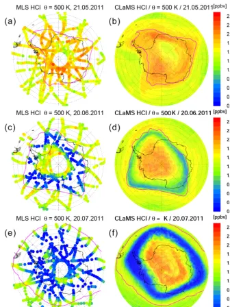
4 Development of HCl in polar stratospheric winter The development of HCl in polar stratospheric winter is strongly influenced by heterogeneous chlorine activa-tion. The heterogeneous reactions that cause this typi-cally occur below a temperature threshold of about 195 K on cold binary aerosol or on PSCs composed of either HNO3/H2SO4/H2O STS solution, water ice or crystalline
NAT. An important and fast HCl sink is the heterogeneous reaction ClONO2+HCl → HNO3+Cl2 (Solomon et al.,
1986). At the beginning of winter, as temperatures drop be-low the threshold for heterogeneous reactions to occur, this reaction quickly depletes HCl typically until all available ClONO2has reacted, since HCl is usually available in large
excess (Jaeglé et al., 1997). This step is therefore referred to as the “titration step”. After that, since no reaction part-ner is available, HCl mixing ratios would remain constant in the dark in the absence of transport or mixing processes. A further depletion of HCl is only possible if there is a re-action partner. This rere-action partner first needs to be formed, and in addition to ClONO2it could be HOCl which would
then react by the heterogeneous reaction HOCl+HCl →
H2O+Cl2(Solomon, 1999). The resulting geographic
distri-bution HCl and its development over the winter is presented in Fig. 1. The figure shows maps of MLS HCl observations (Froidevaux et al., 2008) and corresponding CLaMS results on the 500 K potential temperature level for selected days in May, June and July. On 21 May, when the HCl depletion due to heterogeneous processing is first apparent, the model seems to represent the observations well. By 20 June, HCl depletion has mainly occurred at the vortex edge, where it is more distinctly pronounced in the observations. The compar-ison on 20 July clearly demonstrates the discrepancy between simulations and observations. The model shows HCl mixing ratios well above 1.5 ppbv in the vortex core, while the MLS observations indicate almost zero values of HCl, within the limits of the total estimated uncertainty of the data.
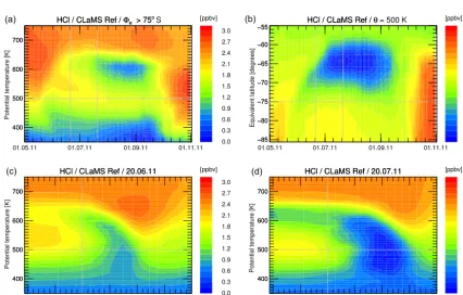
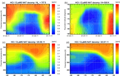
To investigate the HCl discrepancy further, we averaged both the observations and simulation for each day with re-spect to equivalent latitude (Butchart and Remsberg, 1986) and potential temperature using 20 equivalent latitude (8e)
bins of equal area between 8e=50 and 90◦S. Figure 2
shows the characteristics of the observed HCl development by displaying cuts through the equivalent latitude/potential temperature space. Figure 2a shows the time development of the vortex-core average (8e>75◦S) as a function of
poten-tial temperature. Figure 2b shows the time development on the 500 K potential temperature level. Grey lines correspond to the position of the cuts or borders displayed in the other panels. Figure 2c, d show the8e/ θ cross sections for two
selected days, 20 June and 20 July.
Figure 1.Time series of orthographic projection of MLS observations(a, c, e)and CLaMS simulations(b, d, f) of HCl mixing ratios on the 500 K potential temperature level. The maps are shown for 21 May(a, b), 20 June(c, d)and 20 July 2011(e, f). The pink line depicts the edge of the polar vortex according to the criterion of Nash et al. (1996).
the first “titration” step, HCl depletes much more slowly in the simulations compared to the MLS observations. From the comparison of Figs. 2 and 3, it is evident that the model HCl discrepancy is present over a wide altitude range throughout polar winter.
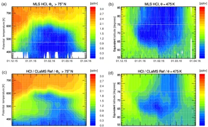
Figure 4 shows the time series of the similarly averaged HCl mixing ratio for the Arctic winter 2015/2016, both for the MLS observations (Fig. 4a, b) and the CLaMS simulation (Fig. 4c, d). This winter was chosen because it was particu-larly cold in the stratosphere (Dörnbrack et al., 2017). Here, the HCl discrepancy is also apparent, although to a lesser
iden-Figure 2.Depiction of MLS HCl mixing ratio data averaged in equivalent latitude/potential temperature space. Panel(a)shows the vortex-core average for equivalent latitudes poleward of 75◦S as a function of time and potential temperature. Panel(b)shows the time development on the 500 K potential temperature level. Panels(c, d)show a snapshot of this average on 20 June and 20 July 2011. Grey lines on the panels indicate the cuts or borders displayed in the other panels of this figure.
[image:7.612.85.511.403.674.2]Figure 4.Similar results as displayed in Figs. 2 and 3 for the simulation of Arctic winter 2016. Panels(a, b)depict the MLS HCl mixing ratio data averaged in equivalent latitude/potential temperature space for the vortex core (8e>75◦N,a) and the time development on the 475 K potential temperature level(b). Panels(c, d)show the corresponding model results from CLaMS. Grey lines on the panels indicate the cuts or borders displayed in the other panels of this figure.
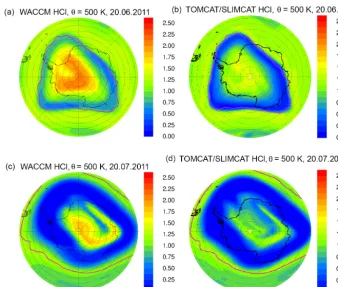
tically as in Fig. 1. The HCl discrepancy is clearly also evident in these simulations, as on 20 July, by when HCl had disappeared in the MLS data; both models also show an area of elevated HCl still present in the polar vortex core, although with lower HCl mixing ratios compared to CLaMS. The HCl depletion in the vortex core is stronger in the TOMCAT/SLIMCAT simulation than in SD-WACCM but still not comparable to the MLS observations. For a more detailed comparison, the results of SD-WACCM and TOMCAT/SLIMCAT have been averaged in 8e/ θ space
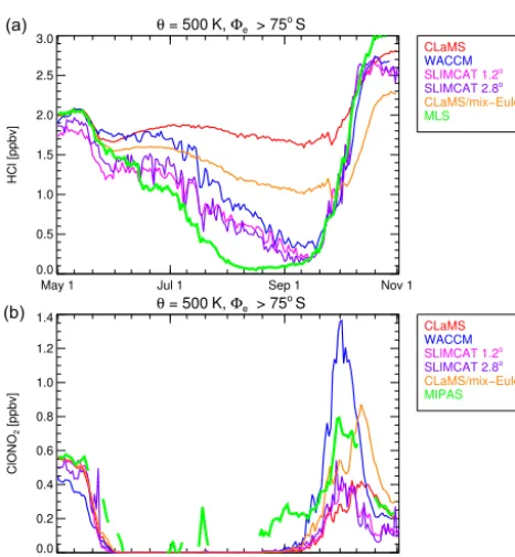
in a similar manner to CLaMS and the observations. The WACCM model daily output interpolated to potential tem-perature levels was averaged using potential vorticity and equivalent latitude calculated from ERA-Interim data. The TOMCAT/SLIMCAT model output was directly averaged within the internal calculated equivalent latitude, also based on ERA-Interim data. A depiction corresponding to Fig. 3 but for SD-WACCM and TOMCAT/SLIMCAT is shown as Figs. S1–S3 in the Supplement. Figure 6 shows a time se-ries of the vortex-core-average HCl and ClONO2simulated
by the three models. The green line corresponds to the MLS and MIPAS observations for HCl and ClONO2, respectively.
However, only very limited ClONO2observations are
avail-able from June to August, since the presence of PSCs im-pedes the MIPAS retrieval process.
There are differences between the individual simulations that arise due to different model formulation and
initiali-sation and that are discussed below. Generally, the Eule-rian models SD-WACCM and TOMCAT/SLIMCAT show a faster HCl depletion than CLaMS. However, it seems that all models underestimate the rate of HCl depletion after the titration step. The three simulations presented show that the initial titration step is completed by the end of May and no further strong changes of HCl occur until early July. Differ-ences during May are likely caused by different initial chlo-rine partitioning. In July and August, HCl decreases further, CLaMS being the model that indicates the slowest HCl de-crease. There is even an apparent HCl increase in CLaMS that is caused by the descent of air masses with higher inor-ganic chlorine Cly.
Figure 5.Simulated HCl from SD-WACCM(a, c)and TOMCAT/SLIMCAT(b, d)on the 500 K potential temperature surface for 20 June
(a, b)and 20 July 2011(c, d) displayed as in Fig. 1.
the differences among the models are unlikely due to model differences in the formulation of the chemical scheme.
A large part of the inter-model difference may be caused by the fact that the Lagrangian formulation of the model CLaMS minimises numerical diffusion while it is inherent in the Eulerian models SD-WACCM and TOMCAT/SLIMCAT. The numerical diffusion arises in Eulerian models because on each time step the chemical tracers are typically averaged within the extent of a model grid box. The minimisation of the numerical diffusion from this lower-resolution limit de-pends on the performance of the advection scheme; for exam-ple, the Prather (1986) scheme used in TOMCAT/SLIMCAT stores subgrid-scale distributions of the tracers. In prac-tice, all Eulerian models likely aim to have tracer advection schemes which limit numerical diffusion, although it will al-ways occur to some extent. The artificial mixing by numer-ical diffusion could provide additional ClONO2or HOCl as
a reaction partner for HCl or NOxthat would form ClONO2.
To investigate this hypothesis, a sensitivity simulation by CLaMS was performed, in which a regular Eulerian grid with 2.8◦×2.8◦ horizontal spacing and the vertical model
grid (with the vertical resolution of 800–1000 m in the lower stratosphere) as vertical levels were defined. Every 24 h of the model run it was checked whether more than one air par-cel resided in the same grid box. These air parpar-cels were then set to the average mixing ratio of all air parcels residing in
the grid box. Although a Eulerian model that must average over these grid boxes on every time step would be even more diffusive, this study can at least show a lower limit of this effect. The corresponding HCl result (labelled “mix-Euler”) is shown as the orange line in Fig. 6. Indeed, the additional imposed Eulerian mixing causes a faster HCl depletion un-til mid-August. Although it is difficult to mimic additional numerical diffusion in a Lagrangian model, this sensitivity supports the assumption that at least part of the difference be-tween CLaMS and the other Eulerian models may be caused by numerical diffusion. Thus, it is likely that the numerical diffusion in the Eulerian models masks part of the effect re-sponsible for the HCl discrepancy investigated in this study. However, it should be noted there is not much difference in the development of HCl between the two resolutions of TOMCAT/SLIMCAT. In the low-resolution simulation, the gradients of ozone and other trace species, especially at the vortex edge, are weaker, but the time series of vortex-core averages are very similar. Potentially, in the high-resolution simulation, the numerical diffusion may already be signifi-cant.
In the following, we list potential model deficiencies that could be responsible for the HCl discrepancy.
1. If the initial ClONO2/HCl ratio was not set to
Figure 6.Vortex-core averages (8e>75◦S) on the 500 K isentrope for HCl(a)and ClONO2(b)for different model simulations. Obser-vations of MLS and MIPAS are shown as green lines. The red line corresponds to CLaMS, the blue line corresponds to SD-WACCM, and pink and purple lines correspond to TOMCAT/SLIMCAT sim-ulations with horizontal resolution 1.2 and 2.8◦, respectively. The orange line corresponds to the CLaMS “mix-Euler” simulation, in which additional artificial mixing was applied.
first titration step of the reaction HCl+ClONO2. This
should have been avoided at least in the CLaMS simu-lations, as both ClONO2and HCl have been initialised
from observations.
2. An error with respect to the transport though the vortex edge or to mixing within the vortex could cause false results. This may affect the results in a similar way to the effect of numerical diffusion discussed above. How-ever, this would likely rather cause a discrepancy near the vortex edge but not in the vortex core.
3. An increased uptake of HCl into PSC particles could be potentially caused by an underestimation of the solu-bility of HCl. As mentioned above, Wohltmann et al. (2017) suggest an empirical correction to resolve the discrepancy in which they apply a−5 K bias within the calculation of the HCl uptake into liquid particles. This correction is able to decrease the HCl discrepancy in the vortex average and is investigated below. However, sig-nificant vertical transport of HCl by particle sedimenta-tion similar to that of HNO3should cause a significant
depletion of total chlorine (Cly) at the end of the polar
winter which is not observed.
Figure 7.MLS observations of HCl mixing ratio on 20 June 2011 in the vortex core (8e>75◦S) on the 500 K potential temperature level. The individual data points are plotted as a function of temper-ature given by ERA-Interim (green symbols). The error bars show the given measurement precision. The corresponding CLaMS re-sults are given as red symbols.
4. There could be unknown heterogeneous chemical reac-tions. Wohltmann et al. (2017) briefly discuss an addi-tional heterogeneous reaction involving HCl and con-clude that this cannot be excon-cluded. However, it must ful-fil the conditions that it does not change the remaining chemical composition to a large extent.
5. A temperature bias of the underlying meteorological analyses would in principle be a possible factor. How-ever, during the period of initial chlorine activation, it would likely not have a significant impact, as the HCl depletion is limited by the availability of ClONO2, not
by the strongly temperature-dependent heterogeneous reaction rate.
6. An offset in the water vapour mixing ratio is another factor. The formation of PSCs and uptake into PSCs depends on the amount of gas-phase water vapour in the model. Therefore, it is also important to verify that the models do not have a significant offset in water vapour mixing ratio. In the case of the CLaMS simula-tion, Tritscher et al. (2018) show that the observed water vapour is well reproduced.
[image:10.612.309.550.66.213.2]5 Characteristics of the HCl discrepancy
To find out more about the characteristics of the potentially missing process that could explain the difference between simulated and observed HCl, we focus on the comparison be-tween simulations and observations for the vortex-core data points on the 500 K level for 20 June (data from about 300 MLS profiles). This is a time and location when, in both the model and the observations, the HCl depletion after the initial titration step is ongoing. From that, we can get hints about the possible missing process (or processes).
First, we investigate whether the missing process is corre-lated with temperature. This would be the case if the deple-tion of HCl is caused by uptake on PSC particles, for exam-ple, into the available liquid PSC particles as suggested by the empirical correction in Wohltmann et al. (2017). Similar to HNO3, HCl is soluble in liquid aerosols. The solubility of
HCl in the liquid aerosols given by the parameterisation of Carslaw et al. (1995) is included in the CLaMS chemistry module. Although the simulations do not show any signifi-cant HCl uptake, it may be that underlying parameters like Henry’s law constant are not accurately represented in the parameterisation as suggested by Wohltmann et al. (2017). The uptake of HCl into the liquid aerosol particles should be strongly temperature dependent (Carslaw et al., 1994), with the largest expected effect for the lowest temperatures. To examine such a hypothesis, the chosen subset of MLS data points and corresponding CLaMS points are plotted as func-tion of temperature in Fig. 7. The temperature for all data points in this subset is below 194 K, suggesting that PSCs should exist at the observation locations shown, which is sup-ported by the MIPAS PSC database (Spang et al., 2018). The simulations and observations in Fig. 6 suggest that the first titration step is completed by 20 June. The temperature de-pendence of the difference between observations and the sim-ulation does not, however, suggest a missing uptake of HCl into the particles. The largest discrepancies between simu-lations and observations are found for higher temperatures. Therefore, the uptake of a significant fraction of HCl into the PSC particles seems to be an unlikely explanation for the dis-crepancy shown between Figs. 2 and 3. However, it cannot be excluded that this dependency is caused by a combination of more than one unknown process.
Although the HCl depletion is not directly correlated with temperature, it seems likely that the missing process should require temperatures low enough for heterogeneous chlorine activation on PSCs or cold aerosols. We examine whether the missing process requires sunlight by investigating the history of the same observed air masses using 30-day back trajecto-ries calculated by the CLaMS trajectory module. From the trajectories, we determined how long the air mass experi-enced sunlight and also how long they were exposed to tem-peratures below 195 K, a typical value below which PSCs can form and heterogeneous chemistry becomes important.
HCl vs. sunlight hours with T<195 K, 20.06.2011, θ = 500 K
0 20 40 60
[image:11.612.308.549.64.214.2]Sunlight time with T < 195 K [h] −0.5 0.0 0.5 1.0 1.5 2.0 HCl [ppbv] MLS CLaMS
Figure 8.MLS observations of HCl mixing ratio that are also dis-played in Fig. 7 plotted against sunlight time with temperatures be-low 195 K derived from the backward trajectories (green symbols) and the corresponding CLaMS results (red symbols).
θ = 500 K; Φe> 75oS
0.0 0.5 1.0 1.5 2.0
HCl [ppbv]
MLS CLaMS −0.04 −0.03 −0.02 −0.01 0.00 0.01 dH C l/d t [ pp bv d
-1] MLS
CLaMS
May 1 Jun 1 Jul 1 Aug 1 0.0
0.2 0.4 0.6 0.8
Fraction of PSC obs
PSCs MIPAS CALIOP CLaMS (a) (b) (c)
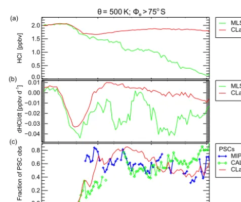
Figure 9.Vortex-core averages (8e>75◦S,θ=500 K) of HCl, its time derivative and PSC occurrence frequency. Panel(a)shows HCl mixing ratios from CLaMS and MLS. Panel(b)shows the cor-responding time derivative dHCl/dt(smoothed as a 6-day running mean). Panel(c)shows the fraction of MIPAS and CALIOP obser-vations with8e>75◦S on the 500 K potential temperature level that are classified as PSCs. It also shows the corresponding CLaMS results. The symbols are connected with coloured lines except for days without PSC information.
Here, we used solar zenith angles below 95◦for the
defini-tion of sunlight time (Rex et al., 2003).
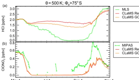
[image:11.612.309.547.292.492.2]Figure 10.Average mixing ratios in the vortex core (8e>75◦S,
θ=500 K) of HCl (a)and ClONO2(b). Green lines show MLS
and MIPAS observations, respectively. CLaMS results are shown for the reference simulation (red) and the simulation with incorpo-rated ionisation from galactic cosmic rays (GCRs, orange).
may both require sunlight and low temperatures in the pres-ence of PSCs.
To further clarify the temporal development of the HCl discrepancy, Fig. 9 shows also the rate of HCl change dHCl/dt calculated from the time series of HCl within the grid box in the equivalent latitude/potential temperature space for each day (Fig. 9b). It is evident that the first titra-tion step caused by the heterogeneous reactitra-tion of HCl with ClONO2is reproduced correctly in the simulation. After that
step, HCl decreases particularly strongly during two periods in mid-June and mid-July. These periods are correlated with a high occurrence fraction of PSCs as shown in Fig. 9c. Both the HCl depletion rate and PSC occurrence seem to have rel-ative maxima around 11 June (i.e. large rate of HCl deple-tion), minima around 23 June and again maxima between 5 and 12 July. The PSC occurrence fraction is shown for both MIPAS and CALIOP observations, which are broadly consis-tent for the overlapping observation times. The correspond-ing CLaMS PSC occurrence fractions are also shown. The only significant difference between MIPAS and CALIOP is in late May where MIPAS detects a large fraction of po-tentially small STS particles that could not be detected by CALIOP. Also in the beginning, these STS detections are pole-centred and therefore partly missed by the limited lat-itudinal coverage of the CALIPSO satellite. The anticorrela-tion between dHCl/dt and the PSC occurrence fraction is a further indication that PSCs may be relevant here. Possible processes missing in the formulation of the model that could explain the HCl discrepancy are investigated in the following section.
6 Potential causes for the HCl discrepancy
The required missing process (or processes) should clearly improve the characteristic difference between observed and
One well-known process that is often neglected in simu-lations of stratospheric chemistry is the ionisation of air molecules by galactic cosmic rays. Galactic cosmic rays (GCRs) provide an additional source of NOxand HOx
(War-neck, 1972; Rusch et al., 1981; Solomon et al., 1981; Müller and Crutzen, 1993). The additional source of OH and NO in the polar stratosphere can trigger an HCl sink through the following reaction chains:
NO+O3→NO2+O2
NO2+ClO M
−→ClONO2
HCl+ClONO2 het
−→Cl2+HNO3
and
OH+O3→HO2+O2
HO2+ClO M
−→HOCl+O2
HOCl+HCl−→het Cl2+H2O.
These reaction chains are only effective in the pres-ence of heterogeneously active particle surfaces (cold binary aerosols or PSCs) and in the presence of sunlight since the ClO molecule would be converted into Cl2 O2 in darkness.
To investigate this effect, the NOx and HOx sources from
cosmic-ray-induced ionisation pairs were incorporated into the chemistry module of CLaMS. The ionisation rate was in-duced after Heaps (1978) using the efficiency effNO=1.25
and effHOx =2 for the formation of NO and OH per
ioni-sation, respectively (Jackman et al., 2016). Fig. 10 shows the corresponding vortex-core average (8e>75◦S) on the
θ= 500 K; Φe>75oS 0.0 0.5 1.0 1.5 2.0 2.5 3.0 HCl [ppbv] MLS CLaMS GCR JHNO3c(NAT)min
JHNO3(NAT)max
May 1 Jul 1 Sep 1 Nov 1
0.0 0.5 1.0 1.5 2.0 2.5 ClONO 2 [ppbv] MIPAS CLaMS GCR JHNO3c(NAT)min
JHNO3(NAT)max
(a)
[image:13.612.47.288.69.207.2](b)
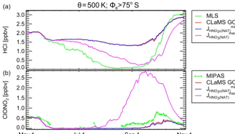
Figure 11.Average mixing ratios in the vortex core (8e>75◦S, θ=500 K) of HCl(a)and ClONO2(b). Green lines show MLS and MIPAS observations, respectively. The red line shows the CLaMS simulation including GCR-induced ionisation. The blue and pink lines correspond to simulations with additional photolysis of partic-ulate HNO3 using the lower and upper estimates, respectively, as described in the text.
6.2 Photolysis of particulate HNO3
Besides the photolysis of gas-phase HNO3, it may be
pos-sible that the HNO3bound in PSC particles also photolyses
directly. Evidence for this comes from studies which have shown that nitrate photolysis from snow surfaces is a signifi-cant source of NOxat the Earth’s surface (e.g. Honrath et al.,
1999; Dominé and Shepson, 2002) and that nitrate photoly-sis in the quasi-liquid layer in laboratory surface studies is enhanced in the presence of halide ions due to a reduced sol-vent cage effect (Wingen et al., 2008; Richards et al., 2011). These studies suggest that photolysis of dissolved HNO3in
PSC particles, including STS droplets, may be possible. If such a process could liberate NOxor HOxinto the gas phase
from the particle phase, it could also cause HCl depletion by the reaction chains mentioned above. However, we note that such a process is not yet proven. Wegner (2013) inves-tigated this hypothesis by implementing this process into the model SD-WACCM. He used the cross section for the NO3−
ion (Chu and Anastasio, 2003), with a quantum yield of 0.3 reflecting relatively high values seen on some surfaces in lab-oratory experiments (Abida et al., 2012). These simulations indicated that due to the low solar elevation in austral win-ters, the onset of HCl depletion in June cannot be reproduced by adding this process. Furthermore, this NOxsource would
cause an overestimation of ClONO2at higher solar elevation
in September.
Here, we extend the investigation by Wegner (2013) by in-cluding possible upper and lower limits for this process, as the photolysis of particulate HNO3 on PSCs has not been
investigated in detail. Laboratory measurements show that combined absorption cross sections of HNO3(aq) and NO3
in bulk solutions are significantly larger than those in the gas phase (Chu and Anastasio, 2003; Svoboda et al., 2013).
θ = 500 K; Φe>75oS
0.0 0.5 1.0 1.5 2.0 2.5 3.0 HCl [ppbv] MLS CLaMS GCR NAT decomp
May 1 Jul 1 Sep 1 Nov 1
[image:13.612.308.549.69.206.2]0.0 0.2 0.4 0.6 0.8 ClONO 2 [ppbv] MIPAS CLaMS GCR NAT decomp
Figure 12.As Fig. 10 but for CLaMS simulation with hypothetical NAT decomposition. CLaMS results are shown for the GCR simu-lation (orange) and the NAT decomp simusimu-lation (blue).
Quantum yields in the aqueous bulk phase are small,≈1 % or less (Warneck and Wurzinger, 1988; Benedict et al., 2017), increasing to a few percent in the quasi-liquid layers (McFall et al., 2018). However, quantum yields on other surfaces may be much larger (Abida et al., 2012), and such large values are also suggested by strong NOx emissions from
nitrate-containing particles exposed to UV radiation (Reed et al., 2017; Ye et al., 2016; Baergen and Donaldson, 2013). As a lower limit for the photolysis of particulate HNO3, we apply
also the gas-phase photolysis of HNO3to the NAT particles
with a quantum yield of 1. As an estimate for the upper limit, we use observations of the absorption cross sections in ice by Chu and Anastasio (2003) and also a quantum yield of 1. The absorption cross sections employed and the photolysis rates derived from those are shown in Fig. S5 of the Supplement. As in Fig. 10, Fig. 11 shows the HCl and ClONO2data, the
CLaMS GCR simulation (blue) and the upper and lower lim-its as described above. The lower limit (blue lines) is not very different from the CLaMS simulation without this process. In the simulation for the upper limit, an additional faster deple-tion of HCl is clearly visible. However, throughout the month of June, the effect is not large enough to fully explain the re-maining HCl discrepancy. Furthermore, the simulation indi-cates that this process would significantly enhance the chlo-rine deactivation into ClONO2in late August and
Septem-ber. Therefore, the upper limit simulation appears not to be the process that would resolve the HCl discrepancy. Poten-tially, this process with a lower quantum yield may explain the small discrepancy in ClONO2in September. The
−85 −80 −75 −70 −65 −60 −55 Equivalent latitude [degrees]
400 500 600 700
−85 −80 −75 −70 −65 −60 −55
400 500 600 700 0.0 0.3 0.6 0.9 1.2 1.5 1.8 2.1 2.4 2.7
−85 −80 −75 −70 −65 −60 −55
400 500 600 700
−85 −80 −75 −70 −65 −60 −55
400 500 600 700 0.0 0.3 0.6 0.9 1.2 1.5 1.8 2.1 2.4 2.7 P ot en tia l t em pe ra tu re [K ] P ot en tia l t em pe ra tu re [K ]
[image:14.612.87.509.65.332.2]Equivalent latitude [degrees]
Figure 13.CLaMS simulation results for HCl of the sensitivity NAT decomp simulation averaged in equivalent latitude/potential temperature space displayed as in Figs. 2 and 3.
6.3 Decomposition of particulate HNO3
A similar hypothesis to that described above would be the decomposition of the condensed-phase HNO3by a process
other than photolysis. A more steady decomposition through-out the polar winter could be triggered, for example, by GCRs instead of by photolysis. For this hypothesis, sun-light or at least twisun-light would still be required to form suf-ficient ClO from the decomposition of the nighttime reser-voir Cl2O2. Over the poles especially, secondary electrons
from GCRs that do not have enough energy to decompose air molecules may still be able to interact with HNO3 on
the PSCs. In Fig. 12, the HCl discrepancy in June and July steadily increases with time in the presence of NAT or ice PSCs. To achieve the observed HCl depletion rate on the 500 K potential temperature level, about 1 % of the con-densed HNO3 per day needs to be liberated into the gas
phase. The exact mechanism by which this could occur needs to be clarified, but to investigate the impact of this hypothesis we performed a test simulation in which the HNO3on NAT
is decomposed into NO2+OH at a constant rate of 10−7s−1,
independent of altitude (labelled “NAT decomp”).
Figure 12 shows the simulated HCl mixing ratios in8e/ θ
space. Even though not every detail of the observations is re-produced, it is evident that this simulation reproduces the ob-servations much better than any of the hypotheses discussed above. The rate of the hypothetical process was chosen such that the HCl depletion on the 500 K level is well represented.
O , 3 Φ e> 60.6 S, 01.10.2011o
0 1 2 3 4 5 6
Ozone [ppmv] 400
500 600 700
Potential temperature [K]
CLaMS GCR NAT decomp SD−WACCM TOMCAT/SLIMCAT CLaMS O3
pass
[image:14.612.308.562.389.531.2]MLS
Figure 14.Simulated vortex mean ozone profile for 1 October 2011 from MLS (green) and different model runs of SD-WACCM (blue), TOMCAT/SLIMCAT (pink) and CLAMS (GCR, orange). The re-sults from the “NAT decomp” sensitivity simulation are shown as a red dashed line. The grey line corresponds to the CLaMS passive ozone tracer and the difference with the other lines indicates the chemical ozone depletion.
It is evident that above this level this rate should increase. However, it does not seem appropriate to speculate further here.
One further piece of evidence for the hypothesis that a pos-sible NOx source from PSC decomposition exists is given
time development of vortex-core mixing ratios of HCl and ClONO2on the 500 K potential temperature level. The blue
line in the top panel demonstrates that on this level the ob-served HCl depletion is represented by the NAT decomp simulation. The MIPAS observations of ClONO2are
inter-mittent since many observations are blocked by the pres-ence of PSCs. However, the remaining observations indicate low mixing ratios in the range between 0.05 and 0.1 ppbv between late May and late August. These observations are better reproduced by the NAT decomp simulation than both other simulations in which ClONO2is nearly zero between
early June and the end of September. From late August to October, simulations of ClONO2are lower than the
simula-tion. The only sensitivity run that exceeds the observations of ClONO2is that with the upper limit for photolysis of
partic-ulate HNO3which also demonstrates that an additional NOx
source would increase the ClONO2mixing ratio.
The change in chlorine activation by this hypothetical pro-cess may also be visible in a comparison with MLS ClO, for which the model output has to be calculated exactly for the location and local time of the observations. For the area of in-terest defined above (20 June, θ=500 K), the observations in the vortex core are, however, at solar zenith angles such that the ClO mixing ratios are mostly zero within experimen-tal uncertainty. For measurements near the vortex edge, no significant ClO differences are induced by this hypothetical process (compare Figs. S6 and S7 of the Supplement).
The complete fingerprint of the 3-D HCl development sim-ilar to Figs. 2 and 3 is shown in Fig. 13. Although differences remain, this sensitivity experiment simulates the HCl obser-vations much better than any other CLaMS simulation dis-cussed here.
7 Impact on polar ozone depletion
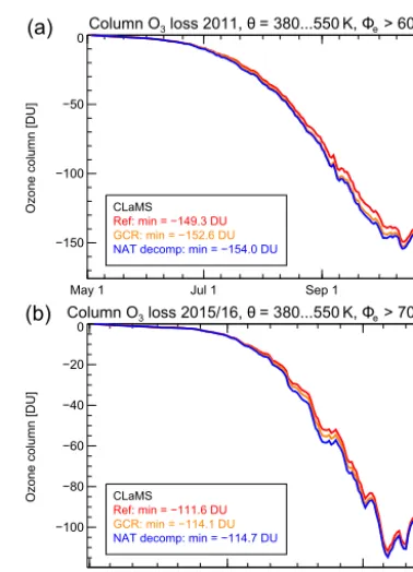
We now investigate the impact of HCl processing on ozone, since the amount of active chlorine in the polar stratosphere is essential for the determination of chemical ozone loss. All three participating models do simulate the chemical ozone loss and the formation of the ozone hole sufficiently well. Figure 14 shows the simulated vortex-average ozone profile on 1 October for the different models in combination with the passive ozone tracer from CLaMS. The difference be-tween the two profiles corresponds to the chemical ozone loss over the winter until this time. The potential process that was included in the NAT decomp simulation increases chlo-rine activation significantly, especially in the polar winter. This might also affect the simulated ozone depletion. How-ever, the difference in chlorine activation is especially large in the rather dark vortex core, where chemical ozone deple-tion rates are small.
The impact of the hypothetical NAT decomposition pro-cesses on polar ozone depletion would cause an additional 0.2 ppmv vortex-average ozone depletion on the 500 K level
Column O3 loss 2011, θ = 380...550K, Φe > 60.6 So
May 1 Jul 1 Sep 1
−150 −100 −50 0
Ozone column [DU] CLaMS
Ref: min = −149.3 DU
GCR: min = −152.6 DU NAT decomp: min = −154.0 DU
Column O3 loss 2015/16, θ = 380...550K, Φe > 70.3 No
Nov 1 Jan 1 Mar 1
−100 −80 −60 −40 −20 0
Ozone column [DU] CLaMS
Ref: min = −111.6 DU
GCR: min = −114.1 DU NAT decomp: min = −114.7 DU
(a)
[image:15.612.332.521.65.327.2](b)
Figure 15.Simulated column ozone loss between 380 and 550 K potential temperature for the Antarctic winter 2011(a)and the Arc-tic winter 2015/2016(b). The results are shown for different sensi-tivity simulations. Red lines correspond to the reference simulation, orange lines to the simulation including GCR-induced ionisation, and blue lines to the NAT decomp simulation. The legend also indi-cates the maximum column ozone loss amount of each simulation.
as shown in Fig. 14. Figure 15 shows the simulated chem-ical ozone depletion for the three CLaMS simulations, the reference simulation, the simulation including GCR-induced ionisation and the simulation also including the hypothetical NAT decomposition. The ozone depletion is also shown for the simulation for the Arctic winter 2015/2016 employing the same model setup. Although it is clear that an increase in chlorine activation yields more ozone depletion, the overall effect on ozone depletion of this additional hypothetical pro-cess is rather low. The increase of column ozone loss in the vortex core due to GCR-induced ionisation ranges from 2 to 3 %. The additional column ozone loss due to the hypotheti-cal NAT decomposition is hypotheti-calculated to be about 1.8 % in the Antarctic winter and only 0.6 % in the Arctic winter.
8 Conclusions
af-have been investigated. The incorporation of GCR-induced ionisation reduces the discrepancy somewhat but is by no means sufficient. The uptake of HCl into PSC particles and photolysis of particulate HNO3also cannot explain the HCl
discrepancy. Simulations with a hypothetical steady decom-position of HNO3 out of NAT PSCs would fit the
require-ments to resolve the HCl discrepancy. This may be caused indirectly by GCRs. At least the observation of elevated ClONO2 observations in late August supports the presence
of an additional NOxsource.
However, at present, the specific process responsible for the HCl decomposition remains unclear. Since the discrep-ancy occurs during the beginning of the chlorine activation period in winter where the ozone loss rates are slow, there is only a minor impact on the overall ozone loss in polar spring.
Data availability. MLS data were obtained from ftp://acdisk.gsfc.
nasa.gov//data/s4pa/Aura_MLS_Level2/, last access: 20 November 2017. MIPAS data are taken from http://share.lsdf.kit.edu/imk/asf/ sat/mipas-export, last access: 8 June 2018. The model data averages on potential temperature surfaces from CLaMS, SD-WACCM, and TOMCAT/SLIMCAT that were used for creating Figs. 2–4, 6, and 9–15 are available from https://datapub.fz-juelich.de/slcs/clams/ hcl_discrepancy/. The CCMI model simulations from SD-WACCM can be requested at https://www.earthsystemgrid.org/search.html? Project=CCMI1. For more detailed model data, please contact the model authors.
The Supplement related to this article is available online at https://doi.org/10.5194/acp-18-8647-2018-supplement.
Competing interests. The authors declare that they have no conflict
of interest.
Special issue statement. This article is part of the special issues
“The Polar Stratosphere in a Changing Climate (POLSTRACC) (ACP/AMT inter-journal SI)” and “Quadrennial Ozone Symposium 2016 – Status and trends of atmospheric ozone (ACP/AMT inter-journal SI)”. It is not associated with a conference.
System Model (CESM), which is supported by the NSF and the Office of Science of the U.S. Department of Energy. Computing re-sources were provided by NCAR’s Climate Simulation Laboratory, sponsored by NSF and other agencies. This research was enabled by the computational and storage resources of NCAR’s Compu-tational and Information Systems Laboratory (CISL). The model output and data used in this paper are listed in the references or available from the NCAR Earth System Grid. We also acknowledge the International Space Science Institute (ISSI) for supporting the Polar Stratospheric Cloud Initiative (PSCi). We are grateful to the European Centre for Medium-Range Weather Forecasts (ECMWF) for providing the meteorological reanalyses. Ines Tritscher was funded by the Deutsche Forschungsgemeinschaft (DFG) under project number 310479827. We thank Michelle Santee and the MLS team, Gabriele Stiller and the MIPAS-Envisat team for the enormous work on providing their high-quality data sets.
The article processing charges for this open-access publication were covered by a Research
Centre of the Helmholtz Association.
Edited by: Bjoern-Martin Sinnhuber
Reviewed by: Ingo Wohltmann and one anonymous referee
References
Abida, O., Du, J., and Zhu, L.: Investigation of the photolysis of the surface-adsorbed HNO3 by combining laser photolysis with Brewster angle cavity ring-down spectroscopy, Chem. Phys. Lett., 534, 77–82, https://doi.org/10.1016/j.cplett.2012.03.034, 2012.
Anderson, J. G., Brune, W. H., and Proffitt, M. H.: Ozone de-struction by chlorine radicals within the Antarctic vortex: The spatial and temporal evolution of ClO-O3anticorrelation based on in situ ER-2 data, J. Geophys. Res., 94, 11465–11479, https://doi.org/10.1029/JD094iD09p11465, 1989.
Baergen, A. M. and Donaldson, D. J.: Photochemical renoxification of nitric acid on real urban grime, Environ. Sci. Technol., 47, 815–820, https://doi.org/10.1021/es3037862, 2013.
Benedict, K. B., McFall, A. S., and Anastasio, C.: Quan-tum yield of nitrite from the photolysis of aqueous ni-trate above 300 nm, Environ. Sci. Technol., 51, 4387–4395, https://doi.org/10.1021/acs.est.6b06370, 2017.
Brakebusch, M., Randall, C. E., Kinnison, D. E., Tilmes, S., San-tee, M. L., and Manney, G. L.: Evaluation of Whole Atmo-sphere Community Climate Model simulations of ozone during Arctic winter 2004–2005, J. Geophys. Res., 118, 2673–2688, https://doi.org/10.1002/jgrd.50226, 2013.
Butchart, N. and Remsberg, E. E.: The area of the stratospheric po-lar vortex as a diagnostic for tracer transport on an isentropic surface, J. Atmos. Sci., 43, 1319–1339, 1986.
Carslaw, K. S., Luo, B. P., Clegg, S. L., Peter, T., Brimble-combe, P., and Crutzen, P. J.: Stratospheric aerosol growth and
HNO3gas phase depletion from coupled HNO3and water
up-take by liquid particles, Geophys. Res. Lett., 21, 2479–2482, https://doi.org/10.1029/94GL02799, 1994.
Carslaw, K. S., Clegg, S. L., and Brimblecombe, P.: A thermody-namic model of the system HCl-HNO3-H2SO4-H2O, including solubilities of HBr, from 328 K to<200 K, J. Phys. Chem., 99, 11557–11574, 1995.
Chipperfield, M. P.: New version of the TOMCAT/SLIMCAT off-line chemical transport model: Intercomparison of strato-spheric tracer experiments, Q. J. R. Meteorol. Soc., 132, https://doi.org/10.1256/qj.05.51, 2006.
Chipperfield, M. P., Lutman, E. R., Kettleborough, J. A., and Pyle, J. A.: Model studies of chlorine deactivation and formation of ClONO2collar in the Arctic polar vortex, J. Geophys. Res., 102, 1467–1478, 1997.
Chipperfield, M. P., Bekki, S., Dhomse, S., Harris, N. R. P., Hassler, B., Hossaini, R., Steinbrecht, W., Thieblemont, R., and Weber, M.: Detecting recovery of the stratospheric ozone layer, Nature, 549, 211–218, https://doi.org/10.1038/nature23681, 2017. Chu, L. and Anastasio, C.: Quantum yields of hydroxyl radical and
nitrogen dioxide from the photolysis of nitrate on ice, J. Phys. Chem. A, 107, 9594–9602, https://doi.org/10.1021/jp0349132, 2003.
Considine, D. B., Douglass, A. R., Kinnison, D. E., Connell, P. S., and Rotman, D. A.: A polar stratospheric cloud parameterization for the three dimensioal model of the global modeling initiative and its response to stratospheric aircraft emissions, J. Geophys. Res., 105, 3955–3975, 2000.
Crutzen, P. J. and Arnold, F.: Nitric acid cloud formation in the cold Antarctic stratosphere: A major cause for the springtime “ozone hole”, Nature, 342, 651–655, 1986.
Dhomse, S. S., Chipperfield, M. P., Feng, W., Hossaini, R., Mann, G. W., and Santee, M. L.: Revisiting the hemispheric asymme-try in midlatitude ozone changes following the Mount Pinatubo eruption: A 3-D model study, Geophys. Res. Lett., 42, 3038– 3047, https://doi.org/10.1002/2015GL063052, 2015.
Dhomse, S. S., Chipperfield, M. P., Damadeo, R. P., Zawodny, J. M., Ball, W. T., Feng, W., Hossaini, R., Mann, G. W., and Haigh, J. D.: On the ambiguous nature of the 11 year solar cycle signal in upper stratospheric ozone, Geophys. Res. Lett., 43, 7241–7249, https://doi.org/10.1002/2016GL069958, 2016.
Dominé, F. and Shepson, P. B.: Air-snow interactions
and atmospheric chemistry, Science, 297, 1506–1510,
https://doi.org/10.1126/science.1074610, 2002.
Dörnbrack, A., Gisinger, S., Pitts, M. C., Poole, L. R., and Ma-turilli, M.: Multilevel Cloud Structures over Svalbard, Mon. Weather Rev., 145, 1149–1159, https://doi.org/10.1175/MWR-D-16-0214.1, 2017.
Drdla, K. and Müller, R.: Temperature thresholds for chlorine acti-vation and ozone loss in the polar stratosphere, Ann. Geophys., 30, 1055–1073, https://doi.org/10.5194/angeo-30-1-2012, 2012. Fahey, D. W., Gao, R. S., Carslaw, K. S., Kettleborough, J., Popp, P. J., Northway, M. J., Holecek, J. C., Ciciora, S. C., McLaugh-lin, R. J., Thompson, T. L., Winkler, R. H., Baumgardner, D. G., Gandrud, B., Wennberg, P. O., Dhaniyala, S., McKinley, K., Pe-ter, T., Salawitch, R. J., Bui, T. P., Elkins, J. W., WebsPe-ter, C. R., Atlas, E. L., Jost, H., Wilson, J. C., Herman, R. L., Kleinböhl, A., and von König, M.: The detection of large HNO3-containing par-ticles in the winter Arctic stratosphere, Science, 291, 1026–1031, 2001.
Farman, J. C., Gardiner, B. G., and Shanklin, J. D.: Large losses of total ozone in Antarctica reveal seasonal ClOx/NOxinteraction, Nature, 315, 207–210, 1985.
Feng, W., Chipperfield, M. P., Davies, S., Mann, G. W., Carslaw, K. S., Dhomse, S., Harvey, L., Randall, C., and Santee, M. L.: Mod-elling the effect of denitrification on polar ozone depletion for Arctic winter 2004/2005, Atmos. Chem. Phys., 11, 6559–6573, https://doi.org/10.5194/acp-11-6559-2011, 2011.
Froidevaux, L., Jiang, Y. B., Lambert, A., Livesey, N. J., Read, W. G., Waters, J. W., Fuller, R. A., Marcy, T. P., Popp, P. J., Gao, R. S., Fahey, D. W., Jucks, K. W., Stachnik, R. A., Toon, G. C., Christensen, L. E., Webster, C. R., Bernath, P. F., Boone, C. D., Walker, K. A., Pumphrey, H. C., Har-wood, R. S., Manney, G. L., Schwartz, M. J., Daffer, W. H., Drouin, B. J., Cofield, R. E., Cuddy, D. T., Jarnot, R. F., Knosp, B. W., Perun, V. S., Snyder, W. V., Stek, P. C., Thurstans, R. P., and Wagner, P. A.: Validation of Aura Microwave Limb Sounder HCl measurements, J. Geophys. Res., 113, D15S25, https://doi.org/10.1029/2007JD009025, 2008.
Garcia, R. R., Marsh, D. R., Kinnison, D. E., Boville, B. A., and Sassi, F.: Simulation of secular trends in the mid-dle atmosphere, 1950–2003, J. Geophys. Res., 112, D09301, https://doi.org/10.1029/2006JD007485, 2007.
Grooß, J.-U., Günther, G., Müller, R., Konopka, P., Bausch, S., Schlager, H., Voigt, C., Volk, C. M., and Toon, G. C.: Simulation of denitrification and ozone loss for the Arctic winter 2002/2003, Atmos. Chem. Phys., 5, 1437–1448, https://doi.org/10.5194/acp-5-1437-2005, 2005.
Grooß, J.-U., Brautzsch, K., Pommrich, R., Solomon, S., and Müller, R.: Stratospheric ozone chemistry in the Antarc-tic: what determines the lowest ozone values reached and their recovery?, Atmos. Chem. Phys., 11, 12217–12226, https://doi.org/10.5194/acp-11-12217-2011, 2011.
K. A., Warneke, T., Wetzel, G., Wood, S., and Zander, R.:
Vali-dation of MIPAS ClONO2measurements, Atmos. Chem. Phys.,
7, 257–281, https://doi.org/10.5194/acp-7-257-2007, 2007. Jackman, C. H., Marsh, D. R., Kinnison, D. E., Mertens, C. J., and
Fleming, E. L.: Atmospheric changes caused by galactic cosmic rays over the period 1960–2010, Atmos. Chem. Phys., 16, 5853– 5866, https://doi.org/10.5194/acp-16-5853-2016, 2016. Jaeglé, L., Webster, C. R., May, R. D., Scott, D. C., Stimpfle,
R. M., Kohn, D. W., Wennberg, P. O., Hanisco, T. F., Cohen, R. C., Proffitt, M. H., Kelly, K. K., Elkins, J., Baumgardner, D., Dye, J. E., Wilson, J. C., Pueschel, R. F., Chan, K. R., Salawitch, R. J., Tuck, A. F., Hovde, S. J., and Yung, Y. L.: Evolution and stoichiometry of heterogeneous processing in the Antarctic stratosphere„ J. Geophys. Res., 102, 13235–13253, https://doi.org/10.1029/97JD00935, 1997.
Kinnison, D. E., Brasseur, G. P., Walters, S., Garcia, R. R., Sassi, D. R. M. F., Harvey, V. L., Randall, C. E., Emmons, L., Lamar-que, J. F., Hess, P., Orlando, J. J., Tie, X. X., Randel, W., Pan, L. L., Gettelman, A., Granier, C., Diehl, T., Niemeier, U., and Simmons, A. J.: Sensitivity of chemical tracers to meteorological parameters in the MOZART-3 chemical transport model, J. Geo-phys. Res., 112, https://doi.org/10.1029/2006JD007879, 2007. Klekociuk, A. R., Tully, M. B., B., K. P., Gies, H. P., Petelina, S. V.,
Alexander, S. P., Deschamps, L. L., Fraser, P. J., Henderson, S. I., Javorniczky, J., Shanklin, J. D., Siddaway, J. M., and Stone, K. A.: The Antarctic ozone hole during 2011, Austral. Meteorol. Ocean. J., 64, 293–311, 2014.
Kunz, A., Pan, L. L., Konopka, P., Kinnison, D. E., and Tilmes, S.: Chemical and dynamical discontinuity at the extratropical tropopause based on START08 and WACCM analyses, J. Geo-phys. Res., 116, https://doi.org/10.1029/2011JD016686, 2011. Kuttippurath, J., Godin-Beekmann, S., Lefèvre, F., Santee, M. L.,
Froidevaux, L., and Hauchecorne, A.: Variability in Antarctic ozone loss in the last decade (2004–2013): high-resolution sim-ulations compared to Aura MLS observations, Atmos. Chem. Phys., 15, 10385–10397, https://doi.org/10.5194/acp-15-10385-2015, 2015.
Lamarque, J.-F., Emmons, L. K., Hess, P. G., Kinnison, D. E., Tilmes, S., Vitt, F., Heald, C. L., Holland, E. A., Lauritzen, P. H., Neu, J., Orlando, J. J., Rasch, P. J., and Tyndall, G. K.: CAM-chem: description and evaluation of interactive at-mospheric chemistry in the Community Earth System Model, Geosci. Model Dev., 5, 369–411, https://doi.org/10.5194/gmd-5-369-2012, 2012.
Calvo, N., and Polvani, L. M.: Climate change from 1850 to 2005 simulated in CESM1(WACCM), J. Climate, 26, 7372– 7390, https://doi.org/10.1175/JCLI-D-12-00558.1, 2013. McFall, A. S., Edwards, K. C., and Anastasio, C.:
Ni-trate Photochemistry at the Air-Ice Interface and in Other
Ice Reservoirs, Environ. Sci. Technol., 52, 5710–5717,
https://doi.org/10.1021/acs.est.8b00095, 2018.
McKenna, D. S., Konopka, P., Grooß, J.-U., Günther, G., Müller, R., Spang, R., Offermann, D., and Orsolini, Y.: A new Chemi-cal Lagrangian Model of the Stratosphere (CLaMS): 1. Formu-lation of advection and mixing, J. Geophys. Res., 107, 4309, https://doi.org/10.1029/2000JD000114, 2002a.
McKenna, D. S., Grooß, J.-U., Günther, G., Konopka, P., Müller, R., Carver, G., and Sasano, Y.: A new Chemical Lagrangian Model of the Stratosphere (CLaMS): 2. Formulation of chem-istry scheme and initialization, J. Geophys. Res., 107, 4256, https://doi.org/10.1029/2000JD000113, 2002b.
Molina, L. T. and Molina, M. J.: Production of Cl2O2from the self-reaction of the ClO radical, J. Phys. Chem., 91, 433–436, 1987. Molina, M. J. and Rowland, F. S.: Stratospheric sink for
chloroflu-oromethanes: chlorine atom-catalysed destruction of ozone, Na-ture, 249, 810–812, 1974.
Molleker, S., Borrmann, S., Schlager, H., Luo, B., Frey, W., Klinge-biel, M., Weigel, R., Ebert, M., Mitev, V., Matthey, R., Woi-wode, W., Oelhaf, H., Dörnbrack, A., Stratmann, G., Grooß, J.-U., Günther, G., Vogel, B., Müller, R., Krämer, M., Meyer, J., and Cairo, F.: Microphysical properties of synoptic-scale polar stratospheric clouds: in situ measurements of unexpectedly large HNO3-containing particles in the Arctic vortex, Atmos. Chem. Phys., 14, 10785–10801, https://doi.org/10.5194/acp-14-10785-2014, 2014.
Morgenstern, O., Braesicke, P., O’Connor, F. M., Bushell, A. C., Johnson, C. E., Osprey, S. M., and Pyle, J. A.: Eval-uation of the new UKCA climate-composition model – Part 1: The stratosphere, Geosci. Model Dev., 2, 43–57, https://doi.org/10.5194/gmd-2-43-2009, 2009.
global models used within phase 1 of the Chemistry-Climate Model Initiative (CCMI), Geosci. Model Dev., 10, 639–671, https://doi.org/10.5194/gmd-10-639-2017, 2017.
Müller, R. and Crutzen, P. J.: A possible role of galactic cosmic rays in chlorine activation during polar night, J. Geophys. Res., 98, 20483–20490, 1993.
Müller, R., Grooß, J.-U., Zafar, A. M., Robrecht, S., and Lehmann, R.: The maintenance of elevated active chlorine levels in the Antarctic lower stratosphere through HCl null cycles, Atmos. Chem. Phys., 18, 2985–2997, https://doi.org/10.5194/acp-18-2985-2018, 2018.
Nash, E. R., Newman, P. A., Rosenfield, J. E., and Schoeberl, M. R.: An objective determination of the polar vortex using Ertel’s po-tential vorticity, J. Geophys. Res., 101, 9471–9478, 1996. Neale, R. B., Richter, J., Park, S., Lauritzen, P. H., Vavrus,
S. J., Rasch, P. J., and Zhang, M.: The mean climate of the Community Atmosphere Model (CAM4) in forced SST and fully coupled experiments, J. Climate, 26, 5150–5168, https://doi.org/10.1175/JCLI-D-12-00236.1, 2013.
Peter, T.: Microphysics and heterogeneous chemistry of polar stratospheric clouds, Ann. Rev. Phys. Chem., 48, 785–822, 1997. Pitts, M. C., Poole, L. R., Dörnbrack, A., and Thomason, L. W.: The 2009–2010 Arctic polar stratospheric cloud season: a CALIPSO perspective, Atmos. Chem. Phys., 11, 2161–2177, https://doi.org/10.5194/acp-11-2161-2011, 2011.
Pitts, M. C., Poole, L. R., Lambert, A., and Thomason, L. W.: An assessment of CALIOP polar stratospheric cloud com-position classification, Atmos. Chem. Phys., 13, 2975–2988, https://doi.org/10.5194/acp-13-2975-2013, 2013.
Pitts, M. C., Poole, L. R., and Gonzalez, R.: Polar stratospheric cloud climatology based on CALIPSO spaceborne lidar mea-surements from 2006– 2017, Atmos. Chem. Phys. Discuss., https://doi.org/10.5194/acp-2018-234, in review, 2018.
Pommrich, R., Müller, R., Grooß, J.-U., Konopka, P., Ploeger, F., Vogel, B., Tao, M., Hoppe, C. M., Günther, G., Spelten, N., Hoffmann, L., Pumphrey, H.-C., Viciani, S., D’Amato, F., Volk, C. M., Hoor, P., Schlager, H., and Riese, M.: Tropical troposphere to stratosphere transport of carbon monoxide and long-lived trace species in the Chemical Lagrangian Model of the Stratosphere (CLaMS), Geosci. Model Dev., 7, 2895–2916, https://doi.org/10.5194/gmd-7-2895-2014, 2014.
Prather, M. J.: Numerical advection by conservation of
second-order moments, J. Geophys. Res., 91, 6671–6681, https://doi.org/10.1029/JD091iD06p06671, 1986.
Reed, C., Evans, M. J., Crilley, L. R., Bloss, W. J., Sherwen, T., Read, K. A., Lee, J. D., and Carpenter, L. J.: Evidence for renoxification in the tropical marine boundary layer, At-mos. Chem. Phys., 17, 4081–4092, https://doi.org/10.5194/acp-17-4081-2017, 2017.
Rex, M., Salawitch, R. J., Santee, M. L., Waters, J. W., Hoppel, K., and Bevilacqua, R.: On the unexplained stratospheric ozone losses during cold Arctic Januaries, Geophys. Res. Lett., 30, 1010, https://doi.org/10.1029/2002GL016008, 2003.
Richards, N. K., Wingen, L.-M., Callahan, K. M., Nishino, N., Kleinman, M. T., Tobias, D. J., and Finlayson-Pitts, B. J.: Nitrate ion photolysis in thin water films in the pres-ence of bromide ions, J. Phys. Chem. A, 115, 5810–5821, https://doi.org/10.1021/jp109560j, 2011.
Rienecker, M. M., Suarez, M. J., Gelaro, R., Todling, R., Bacmeis-ter, J., Liu, E., Bosilovich, M. G., Schubert, S. D., Takacs, L., Kim, G.-K., Bloom, S., Chen, J., Collins, D., Conaty, A., Da Silva, A., Gu, W., Joiner, J., Koster, R. D., Lucchesi, R., Molod, A., Owens, T., Pawson, S., Pegion, P., Redder, C. R., Re-ichle, R., Robertson, F. R., Ruddick, A. G., Sienkiewicz, M., and Woollen, J.: MERRA: NASA’s Modern-Era Retrospective Anal-ysis for Research and Applications, J. Climate, 24, 3624–3648, https://doi.org/10.1175/JCLI-D-11-00015.1, 2011.
Rusch, D. W., Gerard, J. C., Solomon, S., Crutzen, P. J., and Reid, G. C.: The effect of particle precipitation events on the neutral and ion chemistry of the middle atmosphere: I. Odd nitrogen, Planet. Space Sci., 29, 767–774, 1981.
Santee, M. L., MacKenzie, I. A., Manney, G. L., Chipper-field, M. P., Bernath, P. F., Walker, K. A., Boone, C. D., Froidevaux, L., Livesey, N. J., and Waters, J. W.: A study of stratospheric chlorine partitioning based on new satellite measurements and modeling, J. Geophys. Res., 113, D12307, https://doi.org/10.1029/2007JD009057, 2008.
Schoeberl, M. R., Lait, L. R., Newman, P. A., and Rosenfield, J. E.: The structure of the polar vortex, J. Geophys. Res., 97, 7859– 7882, 1992.
Shi, Q., Jayne, J. T., Kolb, C. E., Worsnop, D. R., and Davidovits, P.: Kinetic model for reaction of ClONO2with H2O and HCl and HOCl with HCl in sulfuric acid solutions, J. Geophys. Res., 106, 24259–24274, https://doi.org/10.1029/2000JD000181, 2001. Solomon, S.: Progress towards a quantitative understanding of
Antarctic ozone depletion, Nature, 347, 347–354, 1990.
Solomon, S.: Stratospheric ozone depletion: A review
of concepts and history, Rev. Geophys., 37, 275–316, https://doi.org/10.1029/1999RG900008, 1999.
Solomon, S., Rusch, D. W., Gerard, J. C., Reid, G. C., and Crutzen, P. J.: The effect of particle precipitation events on the neutral and ion chemistry of the middle atmosphere: II. Odd hydrogen, Planet. Space Sci., 29, 885–892, 1981.
Solomon, S., Garcia, R. R., Rowland, F. S., and Wuebbles, D. J.: On the depletion of Antarctic ozone, Nature, 321, 755–758, 1986. Solomon, S., Kinnison, D., Bandoro, J., and Garcia, R.:
Simula-tion of polar ozone depleSimula-tion: An update, J. Geophys. Res., 120, 7958–7974, https://doi.org/10.1002/2015JD023365, 2015. Spang, R., Hoffmann, L., Höpfner, M., Griessbach, S., Müller, R.,
Pitts, M. C., Orr, A. M. W., and Riese, M.: A multi-wavelength classification method for polar stratospheric cloud types us-ing infrared limb spectra, Atmos. Meas. Tech., 9, 3619–3639, https://doi.org/10.5194/amt-9-3619-2016, 2016.
Spang, R., Hoffmann, L., Müller, R., Grooß, J.-U., Tritscher, I., Höpfner, M., Pitts, M., Orr, A., and Riese, M.: A climatology of polar stratospheric cloud composition between 2002 and 2012 based on MIPAS/Envisat observations, Atmos. Chem. Phys., 18, 5089–5113, https://doi.org/10.5194/acp-18-5089-2018, 2018. Stolarski, R. S., Krueger, A. J., Schoeberl, M. R., McPeters, R. D.,
Newman, P. A., and Alpert, J. C.: Nimbus 7 satellite measure-ments of the springtime Antarctic ozone decrease, Nature, 322, 808–811, 1986.