Design selection criteria for discrimination
between nested models for binomial data
T.H. Waterhouse
a, D.C. Woods
b,∗
, J.A. Eccleston
a,
S.M. Lewis
baSchool of Physical Sciences, University of Queensland, Brisbane, QLD 4072,
Australia
bSouthampton Statistical Sciences Research Institute, University of Southampton,
Southampton, SO17 1BJ, UK
Abstract
The aim of an experiment is often to enable discrimination between competing forms for a response model. We consider this problem when there are two com-peting generalized linear models (GLMs) for a binomial response. These models are assumed to have a common link function with the linear predictor of one model nes-ted within that of the other. We consider selection of a continuous design for use in a non-sequential strategy and investigate a new criterion,TE-optimality, based on the
difference in the deviances from the two models. A comparison is made with three existing design selection criteria, namelyT-,Ds- andD-optimality. Issues are raised
through the study of two examples in which designs are assessed using simulation studies of the power to reject the null hypothesis of the simpler model being correct, when the data are generated from the larger model. Parameter estimation for these designs is also discussed and a simple method is investigated of combining designs to form ahybriddesign to achieve both model discrimination and estimation. Such a method may offer a computational advantage over the use of a compound criterion and the similar performance of the resulting designs is illustrated in an example.
MSC:primary 62K05, 62J12; secondary 62K20
Key words: Binary response, Continuous designs, Deviance, D-optimality, Hybrid designs, Likelihood ratio test, Logistic regression,T-optimality
∗ Corresponding author.
Email addresses: [email protected] (T.H. Waterhouse),
1 Introduction
When an experiment results in a binary outcome, the relationship between the
kindependent variablesx1, . . . , xkand the response may be approximated by a generalized linear model (GLM) as described, for example, by McCullagh and Nelder (1989). In such models, the number,Yj, of successes at thejth distinct design point follows a binomial distribution Bin(mj, πj), for j = 1, . . . , n. Further, the success probabilityπj is related to thejth treatment (combination of variable values) xj = (x1j, . . . , xkj)′ through
g(πj) = f(xj)′
β,
where g(·) is the link function and ηj = f(xj)′β is the linear predictor, with
f(xj) aq×1 vector of known functions andβ aq×1 vector of unknown para-meters. Thus the link function relates the success probability,πj, to the linear predictor. Examples of link functions are the logit,ηj = log (πj/(1−πj)); the probit, ηj = Φ−1(πj), where Φ is the normal cumulative distribution func-tion; and the complementary log-log link, η(xj) = log{−log (1−πj)}. It is assumed that observations from an experiment are independent and that a single observation is made on each of the N = Pn
j=1mj experimental units. Also, the units are assumed to be exchangeable in the sense that the distribu-tion of the response to a treatment does not depend on the unit to which the treatment is applied.
Most work in the literature has focused on finding designs for GLMs that allow accurate estimation of the unknown model parameters; see, for example, Firth and Hinde (1997) and Woods, Lewis, Eccleston, and Russell (2005). However, earlier experimentation may aim to choose between two or more models, each of which offers a plausible description of the response. As an example, suppose that two models differ by one or more interaction terms. Then the ability to choose between these alternatives in an early experiment has an important impact on the effective design of subsequent investigations. For such model discrimination experiments, different designs may be required from those for parameter estimation. To find designs for linear or nonlinear models, Atkinson and Fedorov (1975a,b) proposed theT-optimality criterion. They showed that, for two competing models, T-optimal designs lead to the most powerfulF-test for the lack of fit of one arbitrarily chosen model, under the assumption that the other model is “true”. Recent work on designs for model discrimination includes the sequential approach for linear models of Dette and Kwiecien (2004) and methods for multi-response nonlinear models by Uci´nski and Bogacka (2005).
for-mulated the T-optimality criterion in terms of the deviance, where the use of the deviance as a goodness-of-fit test statistic is equivalent to the use of an
F-test for a linear model. A weighted sum of deviances was used by M¨uller and Ponce de Leon (1996a) to find sequential designs for model discrimination for binomial data. They used a simulation study to assess designs for discrimin-ating between GLMs with logit and probit link functions and the same linear predictors. As the logit and probit link functions are almost linearly related over most of their common domain, the problem of discrimination between the corresponding GLMs is usually of less practical importance than that of dis-crimination between models with a common link function and differing linear predictors.
In this paper, we investigate a variety of optimality criteria for choosing designs to discriminate between two nested GLMs for binomial data; that is, between modelsM1 andM2 with the linear predictor forM1 nested within that forM2. We consider the set Ξ of all possible continuous designs, defined by probability measures on X = [−1,1]k, the space of possible design points. Each design ξ has n distinct, or support, points and is represented as
ξ=
x1 x2 · · · xn
w1 w2 · · · wn
,
where the vector xj holds the values of the k variables at the jth support point. The weight wj ∈ [0,1] represents the proportion of the total experi-mental effort expended on the jth support point, so that Pn
j=1wj = 1 (see, for example, Fedorov and Hackl, 1997).
In Section 2 we discuss four criteria for design selection: a T-optimality cri-terion based on deviance,DS-optimality,D-optimality under the larger model,
2 Criteria
The criteria discussed in this section are motivated by two closely related objectives: first, the testing of the assertion that modelM1 is correct (T- and
TE-optimality); secondly, the estimation of some or all of the model parameters in model M2 as accurately as possible (D- and Ds-optimality).
2.1 Deviance-based T-optimality
The deviance is an often-used measure of the goodness-of-fit of a GLM to the observed responses y obtained from design ξ. For model Mi (i = 1,2), it is defined by
Di(ξ,y) = 2l(ξ,y,y)−2l(ξ,πˆi,y), (1)
where ˆπi = (ˆπ1i, . . . ,πˆni)′ is the estimate of π = (π1, . . . , πn)′ obtained by using maximum likelihood estimates of the qi unknown parameters, βi, of model Mi, and
l(ξ,γ,y) =N
n X
j=1
wj[˜πjlogγj+ (1−π˜j) log(1−γj)] (2)
is a log-likelihood function for γ = ˜π or ˆπi, with ˜πj =yj/mj and mj =N wj (j = 1, . . . , n). The maximum value of (2), corresponding to the saturated model, isl(ξ,π˜;y) and is achieved when the estimates and observations coin-cide.
A T-optimal design ξ∗
T for discriminating between models M1 and M2 max-imizes the deviance of M1 when M2 is assumed to be the true model, that is,
D1(ξT∗,µ2) = maxξ∈Ξ D1(ξ,µ2), (3)
see Ponce de Leon and Atkinson (1992). In this equation, µ2 is the vector of expected responses under M2 having jth entry mjg−1(ηj(2)), where η
(i) j is the value of the linear predictor at the jth support point for model Mi (i = 1,2;j = 1, . . . , n). As µ2 depends on the value of β2, ξ∗
A potential disadvantage of T-optimality is that the deviance D1(ξ,Y) may not follow the χ2
n−q1 distribution given by asymptotic theory, particularly for sparse data, see McCullagh and Nelder (1989, p.119-121). A particular concern is that a large deviance is not necessarily evidence against the null hypothesis that the data are adequately described by modelM1. Sparseness may be par-ticularly acute for data from designed experiments (see Woods et al., 2005, for an example) and may also lead to other problems, such as non-convergence of the iterative procedures in maximum likelihood estimation (for example, Firth, 1993).
2.2 TE-optimality
For nested GLMs, a more useful measure of the adequacy of M1 is to test the hypothesis that M1 is the correct model against the alternative that M2 is correct, using the reduction in deviance achieved by fitting M2 to the data compared with fittingM1 (as discussed, for example, by Agresti, 2002, p.141). For a given design ξ, the reduction in deviance is the value of the likelihood ratio test statistic given by
R(ξ,y) =D1(ξ,y)−D2(ξ,y)
= 2{l(ξ,πˆ2,y)−l(ξ,πˆ1,y)} . (4)
Under the null hypothesis, R(ξ,Y) follows asymptotically a χ2 distribution on (q2 −q1) degrees of freedom. For a finite number of support points, this approximation is regarded as being quite accurate for the difference in devi-ance, even though a χ2 distribution may be an inadequate approximation for the deviance itself.
The TE-optimality objective function is the expected value of R(ξ,Y). Thus a designξ∗
TE is TE-optimal if
E{R(ξ∗
TE,Y)}= maxξ
∈Ξ E{R(ξ,
Y)}. (5)
2.3 D- and Ds-optimality
AD-optimal design for a GLM estimates the model parameters with minimum asymptotic generalized variance. Under model Mi (i = 1,2), the objective function is given by
φD(ξ, Mi) =|Xi′WiXi|, (6)
whereXi is then×qi model matrix for Miand Wi is a diagonal weight matrix with (j, j)th element
Wi(j, j) =mj
dπj
dηj !
/[πj(1−πj)], for j = 1, . . . , n .
A design ξ∗
D isD-optimal if
φD(ξD∗, Mi) = maxξ∈Ξ φD(ξ, Mi),
where ξ∗
D is dependent on the parameters of Mi, that is, ξD∗ is only locally optimal. See Firth and Hinde (1997) and Woods et al. (2005) for methods of overcoming this limitation.
TheDs-optimality criterion seeks a design which estimates a particular subset of the parameters of a given model as accurately as possible and hence may be applied to the nested models M1 and M2. In order to find a Ds-optimal design ξ∗
Ds for the additional parameters in M2, the objective function is
φDS(ξ, M1, M2) =|X
∗
2
′
W2X2∗−X
∗
2
′
W2X1(X1′W2X1)−1X1′W2X2∗|,
where X2 = [X1|X2∗] and X
∗
2 is the n×(q2−q1) matrix with columns corres-ponding to the additional parameters in M2. A Ds-optimal design ξD∗s max-imizes this function, that is,
φDS(ξ
∗
Ds, M1, M2) = max
ξ∈Ξ φDS(ξ, M1, M2).
an application of Ds-optimality for probit models in the design of a study in economics.
2.4 Implementation
In order to compare the above criteria, each has been implemented in search algorithms to find designs. For the T-,D- andDs-criterion, the BFGS Quasi-Newton method (Dennis and Schnabel, 1983) was used in the search. To im-plement theTE-criterion, the expectation ofR(ξ,Y) is required, see (5), which is analytically intractable. Hence the objective function was approximated us-ing Monte Carlo simulation (see, for example, Gentle, 2003, ch.7), with the binomial success probability at support point j obtained from independent draws from Beta(uj,vj) distributions, forj = 1, . . . , n. The parametersuj and
vj were chosen to make the mean of the jth Beta distribution equal to the probability of success, π(2)j , under M2 and the variance proportional to the mean. That is,
π(2)j =
uj
uj+vj
and cπ(2)j (1−π (2) j ) =
ujvj
(uj+vj)2(uj+vj + 1)
,
wherec > 0 is a constant of proportionality. When the additional parameters have only small impact on the predicted response, then a small value of c
should be used. This is because it is only possible to distinguish between closely similar models using a prediction-based criterion when negligible noise can be assumed. Note that theT-optimality criterion assumes zero noise. This issue is illustrated in Example 2 of Section 3.
The embedding of Monte Carlo function evaluation within design search al-gorithms has been successful in several areas of design; for example, Hamada, Martz, Reese, and Wilson (2001) and Woods (2005). Our implementation uses a simulated annealing algorithm (see, for example, Spall, 2003, ch.8) which has proved useful in optimizing noisy functions in a wide range of applications. Our algorithm used 1000 independent draws for the success probabilities for every function evaluation in order to achieve satisfactory control of the Monte Carlo error.
3 Comparison of criteria
A method of assessing the effectiveness of the four criteria is to evaluate the designs selected using an estimate of the power of a test of the null hypothesis
the estimate is obtained using data from simulated experiments with a range of experiment sizes. In this section, we apply this method to investigate the criteria on two examples and use the difference in deviance between the two models as a test statistic. A hypothesis test against a specified alternative is preferred to a lack-of-fit test forM1based on the deviance, not only because of the previously discussed unreliable distributional properties of the deviance, but also because of the ambiguity in the number of degrees of freedom for the deviance according to whether the data are viewed as grouped or ungrouped (Davison, 2003, p.491-492).
For each criterion, a continuous design is obtained by search algorithm. An observation is generated for the jth support point as a random draw from a Bin(mj, π(2)j ) distribution, where mj is approximated by integer rounding of
N wj (j = 1, . . . , n). Both models M1 and M2 are fitted to the data set and the difference in deviance is compared with the χ2
(1−α),(q2−q1) percentile. This process is repeated n0 times and the proportion of times that H0 is rejected is recorded.
When the data from the simulated experiments give proportions near 0 or 1, the problem of infinite or unstable parameter estimates may arise. Although this clearly presents a problem for parameter estimation and prediction, it does not necessarily imply a poor fitting model as, usually, the fitted values, and therefore the deviance, converge to their limiting values (McCullagh and Nelder, 1989, p.117). Rather, this problem is indicative of the inability of the models to distinguish between “large” and “very large” values of the linear predictor, and similarly between “small” and “very small” values. These situ-ations result in fitted probabilities of 1 or 0 respectively. This problem is par-ticularly acute for the probit link. When this problem arises in the simulated experiments, we have not excluded fitted models with unstable parameters, as might be considered in an investigation concerning parameter estimation.
The following examples illustrate this method of evaluation and allow com-parison of the criteria. As the T-, D- and Ds-optimality criteria find locally optimal designs, values of the parameters in M2 need to be specified for each example. These parameters are also used to determine the Beta distribution used to evaluate the TE-objective function. The parameters in M1 are not needed, as the D-optimal design is only found for the larger model.
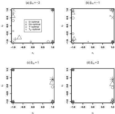
Example 1: Logistic regression with two factors: M1 has an additive linear
predictor with three parameters (q1 = 3); M2 also includes the interaction term (q2 = 4). Thus, the linear predictors are
η(1) =β01+β11x1+β21x2,
−1.0 −0.5 0.0 0.5 1.0 −1.0 −0.5 0.0 0.5 1.0
(a) β32= −2
x1 x2
−1.0 −0.5 0.0 0.5 1.0
−1.0
−0.5
0.0
0.5
1.0
−1.0 −0.5 0.0 0.5 1.0
−1.0
−0.5
0.0
0.5
1.0
−1.0 −0.5 0.0 0.5 1.0
−1.0 −0.5 0.0 0.5 1.0 D−optimal Ds−optimal T−optimal TE−optimal
−1.0 −0.5 0.0 0.5 1.0
−1.0
−0.5
0.0
0.5
1.0
(b) β32= −1
x1 x2
−1.0 −0.5 0.0 0.5 1.0
−1.0
−0.5
0.0
0.5
1.0
−1.0 −0.5 0.0 0.5 1.0
−1.0
−0.5
0.0
0.5
1.0
−1.0 −0.5 0.0 0.5 1.0
−1.0
−0.5
0.0
0.5
1.0
−1.0 −0.5 0.0 0.5 1.0
−1.0
−0.5
0.0
0.5
1.0
(c) β32=1
x1 x2
−1.0 −0.5 0.0 0.5 1.0
−1.0
−0.5
0.0
0.5
1.0
−1.0 −0.5 0.0 0.5 1.0
−1.0
−0.5
0.0
0.5
1.0
−1.0 −0.5 0.0 0.5 1.0
−1.0
−0.5
0.0
0.5
1.0
−1.0 −0.5 0.0 0.5 1.0
−1.0
−0.5
0.0
0.5
1.0
(d) β32=2
x1 x2
−1.0 −0.5 0.0 0.5 1.0
−1.0
−0.5
0.0
0.5
1.0
−1.0 −0.5 0.0 0.5 1.0
−1.0
−0.5
0.0
0.5
1.0
−1.0 −0.5 0.0 0.5 1.0
−1.0
−0.5
0.0
0.5
[image:9.595.95.467.81.449.2]1.0
Fig. 1. Discrimination designs for four different values of additional parameter β32
in Example 1. The size of each plotted symbol is proportional to the weight assigned to the corresponding support point.
Four choices of parameter values for M2 were investigated, namely β02 = 1,
β12= 1, β22 = 2 andβ32∈ {−2,−1,1,2}.
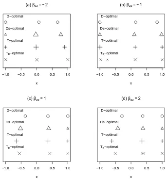
Example 2: Probit regression with one factor:M1 has a first-order linear pre-dictor (q1 = 2);M2is a second order model (q2 = 3). Thus the linear predictors are
η(1) =β01+β11x ,
η(2) =β02+β12x+β22x2.
Again, four choices of parameter values are considered:β02= 1,β12 =−2 and
−1.0 −0.5 0.0 0.5 1.0
(a) β22= −2
x Ds−optimal
D−optimal
T−optimal
TE−optimal
−1.0 −0.5 0.0 0.5 1.0
(b) β22= −1
x Ds−optimal
D−optimal
T−optimal
TE−optimal
−1.0 −0.5 0.0 0.5 1.0
(c) β22=1
x Ds−optimal
D−optimal
T−optimal
TE−optimal
−1.0 −0.5 0.0 0.5 1.0
(d) β22=2
x Ds−optimal
D−optimal
T−optimal
[image:10.595.126.469.80.451.2]TE−optimal
Fig. 2. Discrimination designs for four different values of additional parameter β22
in Example 2. The size of each plotted symbol is proportional to the weight assigned to the corresponding support point.
For each example, a design was found for each of the four criteria and for each of the four values of the additional parameter. The support points for these designs are shown in Figures 1 and 2, with the size of each plotted symbol proportional to the weight assigned to the support point. All the TE-optimal designs were found using c = 0.1, except for the design in Figure 2(c) for which c= 0.01. For this set of parameter values, the random variation in the simulated response with c = 0.1 dominates the differences in the predictions from the two similar models. Hence, the TE-optimality criterion with c= 0.1 produced a degenerate design with all the support points at, or very near to,
0 50 100 150 200 0.0 0.2 0.4 0.6 0.8 1.0
(a) β32= −2
N
Power
0 50 100 150 200
0.0 0.2 0.4 0.6 0.8 1.0
0 50 100 150 200
0.0 0.2 0.4 0.6 0.8 1.0
0 50 100 150 200
0.0 0.2 0.4 0.6 0.8 1.0 D−optimal Ds−optimal T−optimal TE−optimal
0 50 100 150 200
0.0 0.2 0.4 0.6 0.8 1.0
(b) β32= −1
N
Power
0 50 100 150 200
0.0 0.2 0.4 0.6 0.8 1.0
0 50 100 150 200
0.0 0.2 0.4 0.6 0.8 1.0
0 50 100 150 200
0.0 0.2 0.4 0.6 0.8 1.0
0 50 100 150 200
0.0 0.2 0.4 0.6 0.8 1.0
(c) β32=1
N
Power
0 50 100 150 200
0.0 0.2 0.4 0.6 0.8 1.0
0 50 100 150 200
0.0 0.2 0.4 0.6 0.8 1.0
0 50 100 150 200
0.0 0.2 0.4 0.6 0.8 1.0
0 50 100 150 200
0.0 0.2 0.4 0.6 0.8 1.0
(d) β32=2
N
Power
0 50 100 150 200
0.0 0.2 0.4 0.6 0.8 1.0
0 50 100 150 200
0.0 0.2 0.4 0.6 0.8 1.0
0 50 100 150 200
[image:11.595.94.469.82.451.2]0.0 0.2 0.4 0.6 0.8 1.0
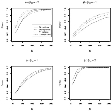
Fig. 3. Power for testingH0 againstHA, against experiment sizeN, for four values
of the additional parameterβ32in Example 1.
designs found from the four criteria. However, the locations differ according to the sign of the additional model parameter in each example.
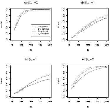
The performances of the 16 designs were compared for each example using the estimated power of the test ofH0againstHAfor experiment sizes ranging from
N = 10 toN = 200 runs. For each experiment, the power was approximated by simulating n0 = 1000 sets of experimental data and performing the test with a significance level ofα = 0.05. Figures 3 and 4 show how the power for each of the designs found from the four criteria is related to the number of runs in the design for Examples 1 and 2, respectively. The curves have been smoothed using a normal kernel smoother (Eubank, 1999, ch.4), with bandwidth equal to 20 and chosen by eye to reduce the impact of Monte Carlo error.
0 50 100 150 200 0.0 0.2 0.4 0.6 0.8 1.0
(a) β22= −2
N
Power
0 50 100 150 200
0.0 0.2 0.4 0.6 0.8 1.0
0 50 100 150 200
0.0 0.2 0.4 0.6 0.8 1.0
0 50 100 150 200
0.0 0.2 0.4 0.6 0.8 1.0 D−optimal Ds−optimal T−optimal TE−optimal
0 50 100 150 200
0.0 0.2 0.4 0.6 0.8 1.0
(b) β22= −1
N
Power
0 50 100 150 200
0.0 0.2 0.4 0.6 0.8 1.0
0 50 100 150 200
0.0 0.2 0.4 0.6 0.8 1.0
0 50 100 150 200
0.0 0.2 0.4 0.6 0.8 1.0
0 50 100 150 200
0.0 0.2 0.4 0.6 0.8 1.0
(c) β22=1
N
Power
0 50 100 150 200
0.0 0.2 0.4 0.6 0.8 1.0
0 50 100 150 200
0.0 0.2 0.4 0.6 0.8 1.0
0 50 100 150 200
0.0 0.2 0.4 0.6 0.8 1.0
0 50 100 150 200
0.0 0.2 0.4 0.6 0.8 1.0
(d) β22=2
N
Power
0 50 100 150 200
0.0 0.2 0.4 0.6 0.8 1.0
0 50 100 150 200
0.0 0.2 0.4 0.6 0.8 1.0
0 50 100 150 200
[image:12.595.96.470.81.452.2]0.0 0.2 0.4 0.6 0.8 1.0
Fig. 4. Power for testingH0 againstHA, against experiment sizeN, for four values
of the additional parameterβ22in Example 2.
occurs for the larger absolute values ofβ32 (Example 1) andβ22 (Example 2). For the more challenging problems, there are greater differences between the performances of the designs, see Figures 3(b) and 4(c), with the D-optimal designs generally having the poorest performance. For every comparison, the
T-optimal design consistently gives the greatest increase in power for increas-ing N. The TE-optimal designs generally have very similar performance to the T-optimal designs, with the power curves virtually indistinguishable in Figures 3(c) and 3(d).
4 Parameter estimation
may not even allow estimation of the parameters in M2, particularly if there is a considerable difference between the two models, such as more than one additional term. In this section, we describe a selection criterion for designs for estimating parameters in two models. We then investigate a method of com-bining designs for discrimination and estimation to provide designs capable of both efficient estimation and discrimination.
4.1 Compound estimation criterion
In order to produce designs for efficient estimation of the parameters in two models, M1 and M2, Atkinson and Cox (1974) suggested maximization of the objective function
φc(ξ, M1, M2) = (φD(ξ, M1))1/q1(φD(ξ, M2))1/q2, (7)
whereφD is defined in (6). This is a special case of the criterion in the seminal work of L¨auter (1974) and has recently been used to find designs for GLMs by Woods et al. (2005).
4.2 Hybrid designs
We considerhybriddesigns which are capable of both discrimination and para-meter estimation. Such a design is formed as a “weighted sum” of a discrimin-ation designξd, such as aT- orTE-optimal design withn
dsupport points, and a design ξe for estimation, such as a design maximizing (7) with n
e support points. A hybrid design ξh is defined as
ξh= (1−a)ξd+aξe
=
xd1 . . . xdnd xe1 . . . xene
(1−a)wd
1 . . . (1−a)wndd aw e
1 . . . awnee
,
where xdj, xel and wd
j, wle (j = 1, . . . , nd; l = 1, . . . , ne) are the support points and corresponding weights of the discrimination and estimation designs re-spectively, and 0 ≤ a ≤ 1. The choice of a allows adjustment of the relative importance of discrimination and estimation: a = 0 gives the discrimination design; a= 1 gives the estimation design.
on compound and constrained criteria which combine the two objectives. The use of hybrid designs offers a computational advantage over these alternative approaches, as it is not required to carry out a separate design search for several values of a in order to investigate designs offering different trade-offs between discrimination and estimation. This is a considerable benefit if a simulation-based criterion, such asTE-optimality, is used for discrimination.
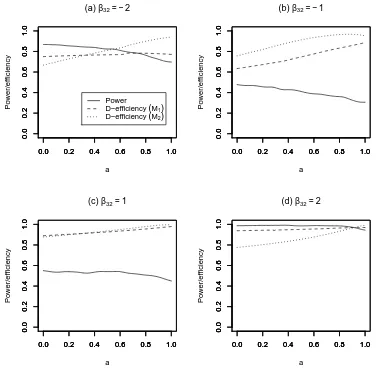
We investigate the performance of hybrid designs formed from a T-optimal design and an estimation design for the models in Example 1. The T-optimal designs are those discussed in Section 3 and the estimation designs were ob-tained by design search through maximization of (7). For 101 equally spaced values of a in [0,1], hybrid designs were assessed through (i) power, as de-scribed in Section 3, with N chosen to be 100, and (ii) through their D -efficiency under modeli, defined as
EffDi = "
φD(ξh, M i)
φD(ξi∗, Mi) #1/qi
,
whereφD is defined in (6) andξi∗ is theD-optimal design under modelMi (i= 1,2). Parameter values forM1 were obtained by fittingM1 to data generated from modelM2 using the T-optimal design. Alternatively, any available prior knowledge of the parameters inM1 could be used.
The results of the investigation are shown in Figure 5, where the curves for power have been smoothed using a kernel smoother with bandwidth equal to 0.1. The trade-off between discrimination and estimation ability as a varies depends upon the difference between the models. When a large difference ex-ists, such as when β32 = 2, high D-efficiency, under both M1 and M2, and high power can be achieved simultaneously through setting a = 0.8, see Fig-ure 5(d). When there is less difference between the models, maximum perform-ance for both estimation and discrimination cannot be achieved and a sub-stantial trade-off between the two requirements is necessary, see Figure 5(b).
4.3 DT-optimality
Atkinson (2005) described the DT-optimality criterion for estimation of, and discrimination between, two or more models with normally distributed errors. We extend this criterion to the comparison of two GLMs,M1 andM2, through use of the objective function
0.0 0.2 0.4 0.6 0.8 1.0 0.0 0.2 0.4 0.6 0.8 1.0
(a) β32= −2
a
Power/efficiency
0.0 0.2 0.4 0.6 0.8 1.0
0.0 0.2 0.4 0.6 0.8 1.0
0.0 0.2 0.4 0.6 0.8 1.0
0.0 0.2 0.4 0.6 0.8 1.0 Power
D−efficiency (M1)
D−efficiency (M2)
0.0 0.2 0.4 0.6 0.8 1.0
0.0 0.2 0.4 0.6 0.8 1.0
(b) β32= −1
a
Power/efficiency
0.0 0.2 0.4 0.6 0.8 1.0
0.0 0.2 0.4 0.6 0.8 1.0
0.0 0.2 0.4 0.6 0.8 1.0
0.0 0.2 0.4 0.6 0.8 1.0
0.0 0.2 0.4 0.6 0.8 1.0
0.0 0.2 0.4 0.6 0.8 1.0
(c) β32=1
a
Power/efficiency
0.0 0.2 0.4 0.6 0.8 1.0
0.0 0.2 0.4 0.6 0.8 1.0
0.0 0.2 0.4 0.6 0.8 1.0
0.0 0.2 0.4 0.6 0.8 1.0
0.0 0.2 0.4 0.6 0.8 1.0
0.0 0.2 0.4 0.6 0.8 1.0
(d) β32=2
a
Power/efficiency
0.0 0.2 0.4 0.6 0.8 1.0
0.0 0.2 0.4 0.6 0.8 1.0
0.0 0.2 0.4 0.6 0.8 1.0
[image:15.595.94.469.82.452.2]0.0 0.2 0.4 0.6 0.8 1.0
Fig. 5. The power andD-efficiency of the hybrid designs of Example 1 for 0≤a≤1.
0.0 0.2 0.4 0.6 0.8 1.0 0.0 0.2 0.4 0.6 0.8 1.0
(a) β32= −2
a
Power/efficiency
0.0 0.2 0.4 0.6 0.8 1.0
0.0 0.2 0.4 0.6 0.8 1.0
0.0 0.2 0.4 0.6 0.8 1.0
0.0 0.2 0.4 0.6 0.8 1.0 Power
D−efficiency (M1)
D−efficiency (M2)
0.0 0.2 0.4 0.6 0.8 1.0
0.0 0.2 0.4 0.6 0.8 1.0
(b) β32= −1
a
Power/efficiency
0.0 0.2 0.4 0.6 0.8 1.0
0.0 0.2 0.4 0.6 0.8 1.0
0.0 0.2 0.4 0.6 0.8 1.0
0.0 0.2 0.4 0.6 0.8 1.0
0.0 0.2 0.4 0.6 0.8 1.0
0.0 0.2 0.4 0.6 0.8 1.0
(c) β32=1
a
Power/efficiency
0.0 0.2 0.4 0.6 0.8 1.0
0.0 0.2 0.4 0.6 0.8 1.0
0.0 0.2 0.4 0.6 0.8 1.0
0.0 0.2 0.4 0.6 0.8 1.0
0.0 0.2 0.4 0.6 0.8 1.0
0.0 0.2 0.4 0.6 0.8 1.0
(d) β32=2
a
Power/efficiency
0.0 0.2 0.4 0.6 0.8 1.0
0.0 0.2 0.4 0.6 0.8 1.0
0.0 0.2 0.4 0.6 0.8 1.0
[image:16.595.94.470.82.452.2]0.0 0.2 0.4 0.6 0.8 1.0
Fig. 6. The power and D-efficiency of the DT-optimal designs of Example 1 for 0≤a≤1.
5 Discussion
When the aim of an experiment is to maximize the probability of rejecting the smaller of two nested models, given data generated from the larger model, there can be advantages in using a design which is optimal for discrimination, rather than one which is optimal under an estimation criterion. In particular, use of a discrimination design may allow a smaller experiment to be used to achieve some specified power.
0.0 0.2 0.4 0.6 0.8 1.0
0.0
0.2
0.4
0.6
0.8
1.0
D−efficiency under M1
a
Efficiency
0.0 0.2 0.4 0.6 0.8 1.0
0.0
0.2
0.4
0.6
0.8
1.0
Hybrid DT
0.0 0.2 0.4 0.6 0.8 1.0
0.0
0.2
0.4
0.6
0.8
1.0
D−efficiency under M2
a
Efficiency
0.0 0.2 0.4 0.6 0.8 1.0
0.0
0.2
0.4
0.6
0.8
1.0
0.0 0.2 0.4 0.6 0.8 1.0
0.0
0.2
0.4
0.6
0.8
1.0
Power
a
Power
0.0 0.2 0.4 0.6 0.8 1.0
0.0
0.2
0.4
0.6
0.8
[image:17.595.109.462.88.452.2]1.0
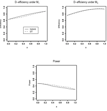
Fig. 7. The performance of hybrid and DT-optimal designs for Example 1 with
β32 = −1, measured by their D-efficiencies under M1 and M2, and the power to
discriminate between the two models.
An important issue in discrimination problems concerns the size of the differ-ence between competing models. If the models are very close, in the sense of producing very similar predictions, then the experimenter needs to consider if there is a scientific need to discriminate between them. If the models are sub-stantially different, then it is unlikely that a tailored design will be necessary to distinguish between them with reasonable power.
An advantage of a TE-optimal design is that it is guaranteed to allow a test of model M1 against M2 using the difference in deviance. Such a test is not guaranteed to be possible for aT-optimal design, particularly when the models differ by more than one term, when theT-optimal design may have insufficient support points for the estimation of M2.
Further research needed in this area includes investigations of methods to overcome the dependence of T-optimal designs on the parameter values for
M2, such as the approach of Ponce de Leon and Atkinson (1991). Another interesting extension is to find designs capable of discriminating between three or more models, as was investigated, for example, by Dette and Kwiecien (2004) for linear models.
Acknowledgements
This research was supported by grants GR/S85139 and EP/C008863 from the Engineering and Physical Sciences Research Council. The first author was supported by an Australian Postgraduate Award. The work benefited from visits by J.A. Eccleston and T.H. Waterhouse to the Southampton Statistical Sciences Research Institute and by S.M. Lewis and D.C. Woods to the Uni-versity of Queensland, with D.C. Woods supported by a grant from the Royal Society.
References
Agresti, A., 2002. Categorical Data Analysis, 2nd Edition. Wiley, New York. Atkinson, A. C., 2005. DT-optimum designs for model discrimination and
parameter estimation. Submitted for publication.
Atkinson, A. C., Cox, D. R., 1974. Planning experiments for discriminating between models (with discussion). Journal of the Royal Statistical Society, Ser. B 36, 321–48.
Atkinson, A. C., Fedorov, V. V., 1975a. The design of experiments for dis-criminating between two rival models. Biometrika 62, 57–70.
Atkinson, A. C., Fedorov, V. V., 1975b. Experiments for discriminating between several models. Biometrika 62, 289–303.
Davison, A. C., 2003. Statistical Models. Cambridge University Press, Cam-bridge.
Dennis, Jr., J. E., Schnabel, R. B., 1983. Numerical methods for unconstrained optimization and nonlinear equations. Prentice Hall Series in Computational Mathematics. Prentice Hall Inc., Englewood Cliffs, NJ.
designs for discrimination between nested regression models. Biometrika 91, 165–176.
Eubank, R. L., 1999. Nonparametric Regression and Spline Smoothing. Marcel Dekker, New York.
Fedorov, V. V., Hackl, P., 1997. Model-Oriented Design of Experiments. Springer, New York.
Firth, D., 1993. Bias reduction of maximum likelihood estimates. Biometrika 80, 27–38.
Firth, D., Hinde, J. P., 1997. Parameter neutral optimum design for non-linear models. Journal of the Royal Statistical Society Ser. B 59, 799–811.
Gentle, J. E., 2003. Random Number Generation and Monte Carlo Methods, 2nd Edition. Springer, New York.
Hamada, M., Martz, H. F., Reese, C. S., Wilson, A. G., 2001. Finding near-optimal Bayesian experimental designs via genetic algorithms. Amer. Stat-istican 62, 175–181.
L¨auter, E., 1974. Experimental design in a class of models. Mathematische Operationsforschung und Statistik 5, 379–396.
McCullagh, P., Nelder, J. A., 1989. Generalized Linear Models, 2nd Edition. Chapman and Hall, New York.
M¨uller, W. G., Ponce de Leon, A. C. M., 1996a. Discrimination between two binary data models: Sequentially designed experiments. Journal of Statist-ical Computation and Simulation 55, 87–100.
M¨uller, W. G., Ponce de Leon, A. C. M., 1996b. Optimal design of an exper-iment in economics. The Economics Journal 106, 122–127.
Ponce de Leon, A. C. M., Atkinson, A. C., 1991. Optimum experimental design for discriminating between two rival models in the presence of prior inform-ation. Biometrika 78, 601–608.
Ponce de Leon, A. C. M., Atkinson, A. C., 1992. The design of experiments to discriminate between two rival generalized linear models. In: L. Fahrmeir, B. Francis, R. Gilchrist (Eds.), Advances in GLIM and Statistical Modelling. Springer, New York, pp. 159–164.
Spall, J. C., 2003. Introduction to Stochastic Search and Optimization. Wiley, Hoboken, NJ.
Uci´nski, D., Bogacka, B., 2005. T-optimum designs for discrimination between two multiresponse dynamic models. J. Roy. Statist. Soc. Ser. B 67, 3–18. Waterhouse, T. H., Eccleston, J. A., 2005. Optimal design criteria for
dis-crimination and estimation in nonlinear models. Tech. rep., University of Queensland, School of Physical Sciences.
Woods, D. C., 2005. Designing experiments under random contamination with application to polynomial spline regression. Statist. Sinica 15, 619–635. Woods, D. C., Lewis, S. M., Eccleston, J. A., Russell, K. G., 2005. Designs