Intelligent Sensors In Software: The Use Of
Parametric Models For Phase Noise Analysis
Arsenia Chorti
∗, Dimosthenis Karatzas
†, Neil M. White
‡, Chris J. Harris
§School of Electronics and Computer Science, University of Southampton, UK, SO17 1BJ
∗ corresponding author: [email protected], †[email protected],‡[email protected], §[email protected]
Abstract
Intelligent senors have attracted particular attention in the recent past. This paper argues that an “intelligent sensor” should be able to perform on-board signal processing within the sensor’s software in order to produce the optimal signal output. A generic intelligent sensor software architecture is described which builds upon the basic requirements of related industry standards. In this framework, advanced signal pro-cessing analyses and algorithms need to be employed. As a case study, we present a novel approach for the analysis of the effect of phase noise in devices such as chemical SAW sensors, gyroscopes, biochemical acoustic wave resonator based sensors and accelerometers.
1. INTRODUCTION
A new generation of sensors, - intelligent sensors - have in recent years become the focus of much research. Advances in fabrication technology in the area of micro-electro-mechanical systems (MEMS) combined with high performance computa-tional capabilities and advanced signal processing algorithms have risen expectations; intelligent sensors should be able to perform self-diagnosis and self-calibration during operation.
In order to identify the functionalities of an intelligent sensor, the IEEE introduced the IEEE1451family of standards [1], [2], [3], [4]. IEEE 1451 provides a formal definition of the basic requirements of an intelligent (or smart) transducer. These standards define the fundamental element of intelligence as the ability to self-identify, and complement this with on board memory and a set of digital, analogue and mixed communication interfaces.
On the other hand, the Self-Validating (SEVA) [5], [6] sensors approach addresses the issue of intelligence at a higher level suggesting that an intelligent sensor should be able to validate its output and associate with it an uncertainty value. Also SEVA proposes a list of pre-defined values that describe a spectrum of diverse sensor conditions that can be used to communicate sensor state information to a higher level. The SEVA approach recently became a British Standard (BS-7986) [7] and is already endorsed by parts of industry.
Following either approach, a central task in the intelligent sensor implementation is the reliable estimation of the noise variance and drift in the circuit output. To perform this tedious task, both parametric and non-parametric approaches
can be employed, based either on a detailed physical model or exclusively on the collected data. We discuss in detail possible implementations based on the Kalman filter algorithm or probability density estimators in [8].
The present paper aims are twofold. Firstly, to outline an intelligent sensor software architecture in accordance with existing standards and which provides enhanced flexibility to meet the requirements of adverse applications. Secondly, in order to illustrate possible advanced signal processing methods that could be employed in such a framework, we perform a case study of the effect of phase noise in sensory systems that include internal oscillators. Such systems are encountered in a variety of applications, ranging from accelerometers and gy-roscopes [9], to SAW chemical sensors [10] and biochemical sensors [11]. A novel parametric analysis for the estimation of drift and phase noise variance in such sensors is presented that lifts the theoretical discrepancies of earlier analyses.
The paper is organized as follows. In section 2 we outline the main functionalities of the intelligent sensor software architecture while in section 3 we describe the particular software modules. Section 4 includes background theory on recent advances in oscillator modeling while we estimate the drift and variance of a sensor that includes a noisy oscillator in section 5. This analysis is prerequisite for the parametric fault detection and drift estimation algorithms described in further detail in [8]. Finally, in section 6 we discuss the conclusions and possible future enhancements of this work.
2. INTELLIGENTSENSORARCHITECTURE
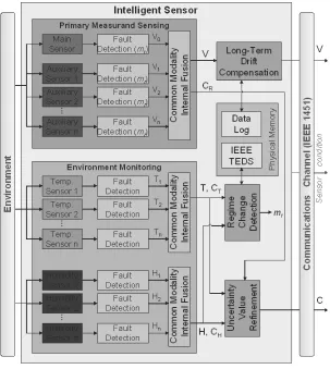
The intelligent sensor defined here comprises a system of indi-vidual sensors and software modules, addressed as a single en-tity. We propose a generic software architecture for intelligent sensors that is compatible with the requirements introduced by IEEE1451to incorporate the following functionalities:
• Real-time fault and drift detection, fault isolation and
signal conditioning.
• Communication of sensor condition to the sensor
man-agement level.
• Adaptation to environmental changes.
Fig. 1: Intelligent Sensor Architecture
the architecture actively advocates redundancy of information and makes use of such redundancy for self validation and reconfiguration. Nevertheless, the design is generic, and the array of primary measurand sensors can reduce (depending on the application) to a single sensor coupled with fault detection module without affecting the functionality, as will be explained later.
The operating environment is monitored by one or more arrays of sensors measuring various environmental attributes (temperature and humidity for the example of Fig. 1). The ex-act number and nature of the attributes observed is dependant on the type of the primary measurand sensors. Each partici-pating sensor is individually monitored by a Fault Detection (FD) module. The outputs of the FD modules in each sensor array are combined by a common modality internal fusion (CMIF) module, which provides a single value and associated uncertainty for each of the measured attributes.
Information about the operating regime is subsequently used to enhance the fault detection process of the primary measurand. To this end, the Regime Change Detection (RCD) module makes use of environmental information to dictate which sensor model should be employed by the fault detection modules of the primary measurand sensors. In addition, the RCD module is able to take immediate action (i.e. shut down
a sensor) to protect the sensing element or issue a warning signal.
Furthermore, knowledge of the environmental conditions is used by the Uncertainty Value Refinement (UVR) module to assess whether the sensor operates within the manufacturer’s recommended conditions and weight the confidence on the measurement accordingly. Finally, the behavior of the intelli-gent sensor at a larger timescale is monitored by the Long-Term Drift Compensation (LTDC) module. The LTDC module identifies and compensates for long-term drift or bias effects typically associated with the ageing of the sensing element.
3. INTELLIGENTSENSORSOFTWAREMODULES A. Fault Detection
Two parallel fault detection processes, namely novelty detec-tion and residual based, run within the fault detecdetec-tion module. The former is a non-parametric fault detection approach while the latter is based on a parametric sensor model.
• Novelty detection determines whether the incoming data
• The residual based scheme, akin to model error prediction
methods, employs Kalman filter error prediction to infer whether the current measurement is likely based on a sliding window of measurement data time history. The information produced by the two parallel processes is subsequently fused within the FD module.
B. Common Modality Internal Fusion
Following fault detection the fault-checked data from like-modality sensors are fused by the Common Modality Internal Fusion (CMIF) module to obtain a single measurement value coupled with an uncertainty value for each of the attributes measured. Assuming that the measurements are drawn from normal distributions, a typical method to perform measure-ment fusion is Optimal Weighting Measuremeasure-ment Fusion [13]. OWMF effectively weights the input of each participating sensor according to the certainty that the corresponding mea-surement is correct (as reported by the related fault detection module).
C. Regime Change Detection
The Regime Change Detection (RCD) module employs envi-ronmental information to ensure that the primary measurand sensor model used by the respective FD modules is correct for the current operating regime. The appropriate sensor model is selected from a library of stored sensor models (computed off-line for the primary measurand sensors) which reside in the physical memory of the intelligent sensor.
In the optimum case scenario, a sensor model is assumed to be valid for the current operating regime. In this case, the RCD module acts as a simple look-up table. Generally though, a particular regime does not necessarily map to a specific pre-defined sensor model. In this case the RCD module constructs a sensor model by interpolating (or extrapolating) existing pre-defined models.
D. Uncertainty Value Refinement
When the sensing element operates outside the manufacturer’s recommended operating conditions or a constructed sensor model is used for fault detection (as opposed to a pre-defined one), the uncertainty on the measurement should be higher and the particular sensor condition should be communicated to the sensor management level. The Uncertainty Value Refinement (UVR) module performs the above tasks.
E. Drift Compensation
Certain sensors, such as CMOS-based sensors, are prone to low frequency effects, such as1/f noise, while chemical sen-sors are often subject to poisoning with time, which adversely affects their sensitivity. The Long-Term Drift Compensation (LTDC) module, aims to detect these drift mechanisms based on the data, and subsequently correct for the introduced measurement bias, effectively elongating the useful life span of the sensor.
In order to estimate and compensate for drift in sensors, we need to account for the underlying generating mechanisms. In
this context, we propose the following classification of drift, according to whether it is correlated to the sensor internal state in a state space representation and whether it is a reversible or irreversible effect:
1) Reversible state dependent drift. It accounts for drift due to sensor non-idelities in the input/output characteristic. Assuming that it is possible to develop a state space model for the sensor, its estimation can be realized using the extended Kalman filter algorithm, as demonstrated in [14].
2) Reversible state independent drift. An example of such drift is the gravitational offset in accelerometers. This kind of drift can generally be estimated (e.g. sensor output when “switched on”).
3) Irreversible state dependent drift.Such drift is the effect of sensor dynamic behavior. The most common example is drift in chemical sensors due to “poisoning”. It can be evaluated through the use of online density estimation algorithms [8].
4) Irreversible state independent drift. This accounts for the effect of low-frequency noise to the sensor output. In this context we will examine in the following section the effect of phase noise in a sensor output.
4. ANALYSIS OF THEEFFECT OFPHASENOISE IN
SENSORS- BACKGROUND ONPHASENOISEMODELING
As mentioned in the previous section it is desirable to be able to implement both parametric and non-parametric algorithms in a fault detection and drift estimation context. Parametric models need to account for the actual physical processes in the device and as a result require extensive experimental and accompanying theoretical models. Whatever the case may be, it is imperative to characterize the main noise sources and their potential effect on the sensor output.
For a large number of sensors their operation is based on internal oscillators and as a result the analysis of their noise performance is translated to the analysis of the phase noise characteristics of noisy oscillatory systems. In this context, two approaches were mainly adopted in literature. The use of the “Allan variance” [15] and the empirical spectral model in-troduced by Leeson [16]. The “Allan’s variance” characterizes the phase noise through the second order empirical moment estimates of first order phase differences. On the other hand, Leeson’s model suggests that the phase noise power spectral density (PSD) of a noisy oscillator is described as a sequence of power law regions of the type
kα
fα, α∈ {0,1,2,3} (1)
wheref represents the deviation from the nominal oscillation frequency.
the research community, especially in what concerns the effect of flicker noise sources in the oscillator loop.
Recently in [17], the aforementioned theoretical problems were overcome using the correlation theory of frequency fluctuations. A novel enhanced oscillator spectral model was derived that accounts for all the main types of power law phase noise and whose parameters can be readily evaluated from trivial macroscopic spectral measurements. More specifically, the proposed model is based on the following observations:
i Phase noise can be efficiently approximated as the sum of power-law processes resulting from integration of frequency fluctuations. At relatively high frequencies where the “small angle approximation”1 is valid the
oscillator PSD coincides with the phase noise PSD. ii A band-limited white-like phase noise component is
expected to generate a weak tone on the oscillator fre-quency added to a band-limited white-like noise region. iii Flicker phase noise of |f|−1−ν PSD results in a finite
variance noise process. The dominant side-band spectral component follows ak1|f−1−ν|characteristic, while the
PSD on the carrier frequency is finite.
iv Long correlated events in the oscillator phase will gen-erate Gaussian-like components in the oscillator PSD.
1/|f|3 and1/f4 phase noise are such processes. v Short correlated events in the oscillator phase give rise
to Lorentzian2-like components in the oscillator PSD.
1/f2 phase noise is such a process.
vi Long correlated events tend to dominate on the near-carrier regime.
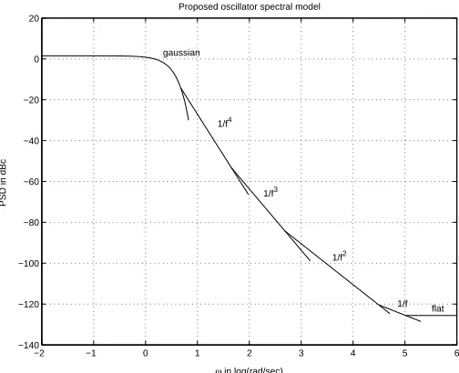
The proposed enhanced oscillator model includes:
1) A Gaussian3-like region near the carrier frequency, as
an approximation of the convolution of the near-carrier sub-spectra.
2) A sequence of power-law regions, in accordance with the small angle approximation.
The model is depicted in Fig. 2 and assumes that the oscillator can be treated as a wide sense stationary random process and that flicker phase noise sources generate finite variance noise terms.
In the following section we will use the enhanced oscillator spectral model to provide estimates of the drift and noise variance in the output of a sensor whose operation is based on internal oscillators.
5. ESTIMATION OFDRIFT ANDPHASENOISEVARIANCE
DUE TOPHASENOISE
As discussed previously, real oscillators suffer from phase noise that distorts the system short-term and long-term stabil-ity. In subsection 5-A we derive in parametric form the amount of drift in the output of such a sensor, while in subsection 5-B we will demonstrate the evaluation of noise variance. Finally
1The small angle approximation states thatejφ'1 +jφwhenφ¿1 2Lorentzian is the shape of the power spectrum of a first order low-pass
filter
3Also known as Doppler lineshape
−2 −1 0 1 2 3 4 5 6
−140 −120 −100 −80 −60 −40 −20 0 20
Proposed oscillator spectral model
ω in log(rad/sec)
PSD in dBc
1/f4
1/f3
1/f2
[image:4.612.315.567.56.261.2]1/f flat gaussian
Fig. 2: Oscillator PSD with Gaussian characteristic near the oscillator frequency
in subsection 5-C we demonstrate the use of the approach on real published data.
A. Drift Estimation
In order to quantify the resulting drift effect, we begin with considering the complex valued oscillation:
ψ(t) =ej(ωosct+φ(t)) (2) where ψ(t) is an analytic version4 of a real oscillator at
ωosc = 2πfosc assuming negligible amplitude noise. In [17]
the correspondence in terms of mean and variance between a real valued oscillator and its complex valued counterpart (analytical representation) is provided. In (2) we can isolate the effect of the phase noise component as a multiplicative term b(t),
b(t) =ejφ(t) (3)
withφ(t)representing the phase noise process. Modelingφ(t)
as a zero-mean Gaussian random process, we can estimate the expected value of the processb(t)as a function of the variance σ2
φ(t)of the phase noise processφ(t):
E£b(t)¤=E£ejφ(t)¤=e−σ
2
φ(t)
2 (4)
where E[·] represents the expected value. (4) expresses the actual drift in the oscillator output.
As a result, drift in the output of oscillatory systems cor-rupted by phase noise is expressed as a function of the overall variance of the phase noise process and can be time dependent in the case of non-stationary phase noise (in which caseσ2
φis
a function of time). The above result can be incorporated in a drift estimation context as well as in the design process of sensors based on oscillators and can be particularly useful in early simulation stages.
4The real oscillator and the complex oscillator are related through the
B. Phase Noise Variance Estimation
The spectral modeling of the noisy oscillator we presented in section 4 is based on macroscopic measurements of the output PSD at frequencies higher from the nominal oscilla-tion frequency (reliable measurements cannot be taken very close to the oscillation frequency). In order to understand the generation mechanism of the near-carrier phase noise we start from the following observations: (i) in the oscillator internal loop noise components at frequencies close to the oscillation frequency (rule of thumb: lower than the half-rate frequency of the oscillation) will be frequency modulated. (ii) Noise components at higher frequencies will be phase modulated.
As a result:
• White noise sources that are phase modulated in the
oscillator loop result in a white noise region at the oscillator output.
• 1/f noise sources that are phase modulated in the
os-cillator loop will generate flicker noise at the osos-cillator output.
• The frequency modulation of white noise sources
gener-ates a 1/f2 region in the oscillator output.
• Frequency modulation of flicker noise generates 1/f3
phase noise.
• The frequency modulation of1/f2noise generates a1/f4
region.
The lower knee frequency of transition from the deep-into-the-carrier to the power law region can be readily evaluated using the above model and the oscillator one-sided PSD at a frequency offset f from the oscillation frequency is given in closed form below:
S(f) = √1
2πΩe
−2πΩ22f2Π(f,0, f4) +k4
f4Π(f, f4, f3)
+ k3
|f|3Π(f, f3, f2) + k2
f2Π(f, f2, f1)
+ k1
|f|Π(f, f1, f0) +k0Π(f, f0, B) (5)
wherefi,i= 0,1,2,3,4are the knee frequencies between the
relevant power law regions,Ωis the variance of the Gaussian region andBstands for the bandwidth of the oscillator. These parameters can be readily evaluated based on the fact that the overall oscillator power is conserved and that the PSD is a continuous function at the knee frequencies. Finally, the functionΠ(x, xl, xu)represents the window function:
Π(x, xl, xu) = ½
1, xl≤x≤xu
0, otherwise
Non-existing regions in the oscillator PSD should simply be suppressed in (5). In the absence of 1/f4 and1/f3 regions, the deep-into-the-carrier region is Lorentzian and the sensor output PSD can be expressed as follows:
S(f) = k2
π2k2+f2Π(f, f2, f1) + k1
|f|Π(f, f1, f0)
+ k0Π(f, f0, B) (6)
In the following we provide an illustration of the use of the described spectral model for phase noise analysis.
C. Case Study: Biochemical Sensor Based on Acoustic Wave Resonators [11]
In [11], a biochemical sensor based on interface biochemistry using a film bulk acoustic wave resonator is presented. The sensor detects mass differences on a biochemically prepared surface that translates them into changes in the output os-cillation frequency. A phase noise analysis of the sensor is performed and it was found that at a frequency offset in the region from 1 kHz to 10 MHz from the oscillation frequency, the PSD followed ak2/f2characteristic. Based on the information available, a Lorentzian region is enough to describe the given sensor PSD.
From the measurements provided in Fig. 8 in [11], we can estimate the PSD parameters. We have that at a frequency offset f = 1000 Hz, the phase noise level is −80 dBc/Hz. Therefore, the coefficientk2characterizing the Lorentzian type PSD of the sensor is evaluated as:
k2
(103)2 = 10
−8⇒k2= 0.01 (7) According to the provided measurements, the sensor output noise is generated from Brownian motion phase noise with PSD as given below:
S(f) = k2
π2k2+f2 ∼=
0.01
0.1 +f2 (8)
The phase noise variance relative to the carrier power can be evaluated as the integral of (8) in the offset frequencies region of interest.
6. CONCLUSIONS
The present paper presents an intelligent sensor software architecture and discusses a novel parametric approach for phase noise analysis in sensory systems. We show that it is possible to incorporate the requirements of existing standards in the area of intelligent transducers using a module based approach for the hardware implementation of the fundamental components of “intelligence” . Furthermore, we present an evaluation of the drift and noise variance in sensors whose operation is based on internal oscillators. It is the goal of the authors to create a wide library of algorithms, both parametric and non-parametric to perform fault detection and drift estimation as discussed in the paper for a variety of sensors and to build a prototype of the intelligent sensor.
REFERENCES
[1] IEEE,IEEE Std 1451.1-1999 Standard for Smart Transducer Interface for Sensors and Actuators - Network Capable Application Processor, J. C. Edison, Ed. Piscataway, NJ: IEEE Standard Association, Apr. 2000.
[3] ——,IEEE Std 1451.32003 Standard for Smart Transducer Interface -Digital Communication and Transducer Electronic Data Sheet (TEDS) Formats for Distributed Multidrop Systems, L. Eccles, Ed. Piscataway, NJ: IEEE Standard Association, Mar. 2004.
[4] ——,IEEE Std 1451.4-2004 Standard for Smart Transducer Interface for Sensor and Actuators - Mixed Mode Communication Protocols and Transducer Electronic Data Sheet (TEDS) Formats, T. Licht, Ed. Piscataway, NJ: IEEE Standard Association, Dec. 2004.
[5] J. Yang and D. Clarke, “A self-validating thermo-couple,”IEEE Trans-actions on Control Systems Technology, vol. 5, no. 2, pp. 239–253, Mar. 1997.
[6] M. Henry, “Recent developments in self-validating (SEVA) sensors,”
Sensor Review, vol. 21, no. 1, pp. 16–22, 2001, emerald Publishing Ltd. [7] B. S. B. 7986:2005,Data Quality Metrics for Industrial Measurement
and Control Systems - Specification. BSi, Apr. 2005.
[8] D. Karatzas, A. Chorti, N. White, and C. Harris, “Teaching old sensors new tricks: archetypes of intelligence,”IEEE Sensors Journal, to appear in the special issue on Intelligent Sensing in fall 2007.
[9] H. Moussa and R. Bourquin, “Theory of direct frequency output vibrating gyroscopes,”IEEE Sensors Journal, vol. 6, no. 2, pp. 310– 315, Apr. 2006.
[10] R. McGill, R. Chung, D. Chrisey, P. Dorsey, P. Matthews, A. Pique, T. Mlsna, and J. Stepnowski, “Performance optimization of surface acoustic wave chemical sensors,”IEEE Transactions on Ultrasonics, Ferroelectrics, and Frequency Control, vol. 45, no. 5, pp. 1370–1380, Sept. 1998.
[11] R. Brederlow, S. Zaumer, A. Scholtz, K. Aufinger, W. Simburger, C. Paulus, A. MArtin, M. Fritz, H. Timme, S. Marksteiner, L. Elbrecht, R. Aigner, and R. Thewes, “Biochemical sensors based on bulk acoustic wave resonators,” in IEEE International Electron Devices Meeting. IEDM 03, Dec. 2003, pp. 3271–3273.
[12] S. Chen, X. Hong, and C. Harris, “Sparse kernel density construction us-ing orthogonal forward regression with leave-one-out test score and local regularization,”IEEE Transactions on Systems, Man, and Cybernetics— Part B: Cybernetics, vol. 34, no. 4, pp. 1708–1717, Aug. 2004. [13] A. Papoulis and S. Pillai,Probability, Random Variables and Stochastic
Processes. New York: McGraw-Hill, 2002.
[14] A. Chorti, D. Karatzas, N. White, and C. Harris, “Use of the EKF for state dependent drift estimation in weakly nonlinear sensors,”Sensor Letters, 2006, in press.
[15] D. Allan and J. Barnes, “A modified ”Allan variance” with increased oscillator characterisation ability,” in Proc. 35th Ann. Freq. Control Symposium, USAERADCOM, Ft. Monmouth, NJ 07703, May 1981, pp. 470–475.
[16] D. B Leeson, “A simple model of feedback oscillator noise spectrum,”
Proceeding Letters of the IEEE, vol. 54, no. 2, pp. 329–330, 1966. [17] A. Chorti and M. Brookes, “A spectral model for RF oscillators with