Economics Division School of Social Sciences University of Southampton Southampton SO17 1BJ UK
Discussion Papers in
Economics and Econometrics
6*''(('%651(5647%674#.4'(14/5 10241&7%6+8+6;#0&241(+6#$+.+6; '0*#0%+0)4'#..1%#6+10'8+&'0%' (41/%1.1/$+#
/CTEGNC'UNCXC ,QJP*CNVKYCPIGT #FTKCPC-WINGT /CWTKEG-WINGT
0Q
The E
ff
ects of Structural Reforms on
Productivity and Pro
fi
tability Enhancing
Reallocation: Evidence from Colombia
∗
Marcela Eslava, John Haltiwanger, Adriana Kugler and Maurice Kugler†
May 24, 2004
Abstract
Estimates for the U.S. suggest that in some sectors productivity en-hancing reallocation is the dominant factor in accounting for producitivity growth. An open question is whether reallocation is always productivity enhancing. Specifically, in developing countries, market concentration, or barriers to competition, may imply that the reallocation process is not fully efficient. Using a unique plant-level longitudinal dataset for Colom-bia for the period 1982-1998, we use plant-level quantities and prices to implement a novel sequential methodology to estimate productivity and demand shocks at the plant level. First, we estimate total factor productivity (TFP) with plant-level physical output data, where we use downstream demand to instrument inputs. We then turn to estimating demand shocks and mark-ups with plant-level price data, using TFP to instrument for output in the inverse-demand equation. Market reforms, introduced in the early1990’s, are associated with rising overall produc-tivity that is largely driven by reallocation away from low- and towards high-productivity businesses. Our evidence also points to allocation of ac-tivity across businesses being less driven by demand factors after reforms.
JEL Classification: F43, L16, O14.
Keywords: Productivity growth, structural reforms, reallocation,
prof-itability, entry and exit.
∗We thank Alberto Serrano, Juan Manuel Contreras and Pablo Medina for excellent
re-search assistance, Alvaro Su´arez and Jos´e Eduardo Granados for providing access to data, as well as seminar participants at DANE, the NBER conference in Chile in November 2003 and, especially, Andy Bernard, Raphael Bergoeing, Jon Eaton, Sebastian Edwards, Mark Roberts and Ernesto Schargrodsky for excellent comments. Support for this project was provided by the World Bank and the IDB. John Haltiwanger also acknowledgesfinancial support from the NSF, Adriana Kugler from the Spanish Ministry of Science and Technology through grant No. SEC-2003-04429, and Maurice Kugler hospitality from the Stanford Center for International Development.
1
Introduction
Market economies are continually restructuring in response to changing condi-tions. The burgeoning evidence from longitudinal micro business databases has shown that productivity growth at the aggregate level is closely connected to the efficiency of the economy at the micro level to allocate outputs and inputs across businesses. That is, a large fraction of measured productivity growth is accounted for by more productive expanding businesses displacing less produc-tive contracting businesses.1
These issues loom especially large in developing economies — although, they have hardly been settled in advanced economies. In developing economies, there are potentially a variety of barriers to promoting efficient ongoing reallocation. These barriers might stem from distortions in market structure as well as the market institutions and policies in place. Aware of the impediments that distor-tionary policies may place on reallocation and, more generally, on productivity growth, during the past decade Latin American countries have undertaken a whole series of reforms (including, labor, financial, and trade reforms) to pro-moteflexibility.
In this paper, we characterize the evolution of the distributions of productiv-ity and other determinants of profitability such as demand factors in Colombia, one of the Latin American economies that underwent extensive structural re-forms in the early nineties. The role of productivity vs. other components of profitability is critical in evaluating the market-oriented reforms in Latin Amer-ica since the reforms were intended to enhance the role of productivity and perhaps reduce the role of demand factors (especially to the extent to which markets were artificially imperfectly competitive) in the allocation of activity. We examine the relationship between the allocation of activity, on the one hand, and productivity and demand factors on the other.2 We then ask how this rela-tionship changed after market reforms were introduced in Colombia in the early 1990’s.
Colombia is a superb country to study these issues for two reasons. First, Colombia underwent a substantial and relatively fast market reform process, mainly in 1990 and 1991. The 1990 labor market reform, which introduced individual severance payments savings accounts, reduced dismissal costs by be-tween 60% and 80% (Kugler (1999, 2004)). The 1991 trade liberalization reduced the average tarifffrom over 62% to around 15% (Lora (1997)). Thefi -nancial reformfirst introduced in 1990 and extended in 1991, liberalized deposit rates, eliminated credit subsidies and modernized capital market and banking legislation (Lora (1997)). In addition, restrictions on inflows of foreign direct in-vestment (FDI) were removed in 1991 as multinationalfirms were given national
1For the labor market, the efficient churning of businesses implies a need to reallocate jobs
at a high pace without long and costly spells of unemployment. The latter is important for not only productive efficiency of the economy but also obviously important for welfare.
2In our analysis, we focus on some of the main determinants of profitability, including
productivity, demand and output prices. There are other determinants of profitability, such
treatment (Kugler (2000)). The 1993 social security reform allowed voluntary transfers from a pay-as-you-go system to a fully-funded system with individual accounts, though it increased employer and employee pension contributions up to 13.5% of earnings (Kugler and Kugler (2003)).
Second, Colombia has unique longitudinal microeconomic data on busi-nesses. A unique feature of the Colombian data is that both plant-level quan-tities and prices can be measured. The ability to measure plant-level prices of both outputs and inputs is potentially very important in this context for both measurement and conceptual reasons. Much of the existing literature measures establishment output as revenue divided by a common industry-level deflator. Therefore, within-industry price differences are embodied in output and pro-ductivity measures. Moreover, if prices reflect idiosyncratic demand shifts or market power variation rather than quality or other differences in product at-tributes, then high “measured” productivity businesses may not be particularly efficient. In this sense, the relationship between productivity and reallocation in the literature may be misleading.3
In the context of a developing economy undergoing structural reforms these measurement and conceptual issues are especially important. A key objective of structural reforms is to make markets more competitive. Without the ability to measure plant-level prices it is very difficult to quantify and, in turn, analyze the respective contributions of demand and efficiency factors in the allocation of activity and how they may have changed in response to market reforms. In this paper, we attempt to measure the separate influences of idiosyncratic productivity and demand on the allocation of activity in Colombia.
In exploiting these unique micro data, our paper makes a number of re-lated methodological innovations relative to much of the literature. First, in measuring efficiency we estimate production functions using an extension of the instrumental variable approach pioneered by Shea (1993) and Syverson (2003). In the latter, Syverson uses local downstream demand instruments to estimate returns to scale of production functions. Building on this approach, we use downstream demand instruments as well as plant-level input prices for materi-als and energy as instruments in estimating production functions. From this structural estimation of production functions, we generate measures of plant-level efficiency (i.e., plant-level total factor productivity). Second, since we can measure plant-level output prices, we estimate demand elasticities using the total factor productivity estimates as instruments in the demand equations. That is, wefirst use downstream demand instruments to estimate production functions and then use supply shocks (i.e., total factor productivity) to estimate
3Since Marschak and Andrews (1944), there has been awareness about the possible
difficul-ties involved in using revenue-based deflated output in establishment level data. Klette and
Griliches (1996) consider how intra-industry pricefluctuations can affect production function
the demand functions.
Having estimated production and demand functions, we study the evolu-tion of the distribuevolu-tions of total factor productivity, demand shocks, and prices through the market reforms in Colombia. Wefind that aggregate TFP is higher after the reforms. Moreover, the dispersion of TFP also rises after the reforms. Our main focus though is on the allocation of activity and its relationship to TFP and demand shocks in Colombia throughout the entire period as well as during periods prior to and subsequent to the reforms. Overall, we find that the allocation of activity reflects both efficiency and demand factors. That is, market shares are higher for businesses that are more efficient and face higher demand. Following the reforms, we find that efficiency factors become more important in the allocation of activity across businesses while demand factors become less important. Interestingly, we find that the rising aggregate pro-ductivity in Colombia over this period is accounted for almost entirely by the improved allocation of activity across businesses.
At the extensive margin, we also find that exiting businesses are less effi -cient and face lower demand for their products relative to incumbents. On the other hand, entering businesses are more efficient than incumbents and exiting businesses, but also face lower demand relative to incumbents. This finding points to the importance of vintage technology relative to learning to account for productivity dynamics. Note that revenue-based TFP measures spuriously include a demand component and thus underestimate technical efficiency of en-trants, who have to build a consumer base, relative to incumbents, who have a established clientele. Hence, the analysis in the present paper provides a better basis to discern between vintage and learning explanations for dynamics and heterogeneity in productivity.
How did these patterns change in response to the market reforms? Af-ter the market reforms, the positive gap between the productive efficiency of the average incumbent and the average exiting business rises but the positive gap between the productive efficiency of the average entering business and the average incumbent declines. On net, the contribution of entry and exit to aver-age productivity rises slightly. Moreover, when we investigate a more dynamic specification we find that, after the reforms, entrants exhibit slightly higher productivity than incumbents . There is also evidence of learning effects in the post-reform period. Putting these pieces together suggests market reforms yielded a more heterogenous group of entrants but that conditional on survival the post- reform entrants contribute more to productivity. Increased learn-ing by enterlearn-ing businesses after the reforms may be due to increased access to new imported capital vintages and increased access to know-how from foreign businesses. These patterns are also consistent with greater selection by the mar-ket of the least productive and profitable businesses after foreign competition was increased, access to subsidized credit was reduced, and dismissal costs were lowered following the reforms.
charac-terizing the positive implications of market reform rather than the normative implications. There are several interesting complicating factors in considering welfare implications. For one, the market power offirms may derive from eco-nomic fundamentals or from institutional factors. For example, it may be that market power derives from product differentiation by each producer and that markets are best characterized by monopolistic competition. The exploitation of market power in this context byfirms still generates a welfare loss with prices being above marginal cost, but even in the absence of markups substantial price heterogeneity across firms would still be a feature of a first-best equilibrium. Alternatively (or in addition), market power may derive from institutional bar-riers (e.g., trade restrictions). Simple intuition suggests that elimination of such barriers will improve welfare, but even here one should be cautious given po-tential second-best considerations. Another related complicated factor is that market power may play an important role in product and process innovations that lead to technological progress. In some creative-destruction models of in-novation and growth (e.g., Aghion and Howitt (1992)), market power plays an important role for innovators in an environment in which there arefixed costs of innovation. We do not have much to say directly about this latter class of models since we do not directly investigate the role of product and process innovation. Part of the reason for this is that our empirical focus is on oper-ating plants in manufacturing (not R&D facilities). Our analysis has more to say about heterogeneity resulting from differences in adoption rather than in-novation. However, a long standing issue in the empirical innovation literature is how much innovation occurs in R&D facilities and how much occurs on the factoryfloor.
The rest of the paper proceeds as follows. Section 2 describes the Colombian context and the market reforms undertaken during the period of study. Section 3 describes the unique data we use in this analysis. Section 4 describes our methodology for estimating plant-level total factor productivity and demand shocks, and presents the results of these estimations. Section 5 describes basic patterns of productivity, demand, and prices in terms of dispersion and persis-tence. Section 6 examines the relations between efficiency and demand, on the one hand, and the allocation of activity, on the other hand, both before and after the reforms. Section 7 provides concluding remarks.
2
Market Reforms in Colombia
effort to control internal strife associated with violent activities of both illicit drug cartels and guerrilla groups. The absence of an economic crisis meant that there was no clear consensus for the need of market-oriented reforms, but at the same time good economic conditions were initially an asset as distributive
con-flict was addressed by elaborate resource transfer schemes (see, e.g. Kugler and Rosenthal (2003)). However, the inability to reconcile market oriented reforms with the continued and pervasive need for redistribution to compensate losers meant that by 1993 the spurt of reform of the early nineties came to a halt. Although there was no reversal of reforms, Colombia did not make additional progress in terms of further removing distortions while many other countries in Latin America, and around the world, actually deepened reform efforts (see, e.g., Burki and Perry (1997)). The fact that the structural reform process in Colombia was a one-offphenomenon aids our identification strategy in trying to assess its impact on the relation between reallocation and productivity.
Before Gaviria’s administration, the government of President Virgilio Barco made some partial progress in trade liberalization but did not gain any signif-icant ground in removing other distortions. The gradual decrease in tariffs initiated by Barco was accelerated by Gaviria after June 1991. By the end of 1991, nominal protection reached 14.4% and effective protection 26.6%, down from 62.5% a year earlier, while 99.9% of items were moved to the free import regime. These measures clearly generated unrest among the owners of capital, who faced lower profit margins after trade liberalization due to increased foreign competition. The impact from market penetration by foreign exporters, and by foreign investors as pointed out below, on the market participation of domestic businesses in product markets was mitigated by more favorable conditions in factor markets, which lowered both capital and labor costs. In labor markets, Law 50 of December 1990 promoted theflexibilization of contracts and reduced labor costs by between 60% and 80% (see, e.g., Kugler (1999, 2004)) . In 1990, the government also tried to introduce changes in the social security system as part of the labor reform package, but Congress forced an independent process to reform pension provision. The opposition to the original reform plan by the Executive stemmed partly from the proposal to lower labor costs by reducing employer’s contributions. Later during the Gaviria administration, the execu-tive compromised with Congress by passing Law 100 in 1993. Although Law 100 allowed for voluntary individual conversion from a pay-as-you-go system to a fully-funded system with accounts, this law also introduced a mandatory hike in employer and employee contributions up to 13.5% of salaries, of which 75% was paid by employers (see, e.g., Kugler and Kugler (2003)).
extent of capital controls. Finally, Resolution 49 of 1991 eliminated restrictions to foreign direct investment. This resolution established national treatment of foreign enterprises and eliminated limits on the transfer of profits abroad as well as bureaucratic procedures requiring the approval of individual projects (see, e.g., Kugler (2000)). This measure not only facilitated capital inflows across all sectors, but also induced entry of foreign banks increasing competition in the
financial sector, thereby yielding lower intermediation costs.
After the end of Gaviria’s term, in 1994 President Ernesto Samper gained power on a platform partially based on opposition to market institutions.4
While the new government was unsuccessful in terms of dismantling existing reforms, the coalition supporting the new government managed to bring the momentum for additional reforms to a halt.
Overall, though, the reform process was relatively smooth and successful in transforming a highly distorted economy into one burdened with many fewer frictions. Trade liberalization and the removal of FDI restrictions were aimed at increasing competition and shifting production away from low- and towards high-productivity businesses. In addition, the liberalization of factor markets had the purpose of facilitating reallocation in the economy after the structural reform process. If the goal of inducing productivity-enhancing reallocation was achieved, its success should be reflected in different patterns of industrial dynamics between the 1980’s and the 1990’s, with market allocation being driven to a large extent by productivity rather than profitability in the latter period. In the following sections, we investigate whether this is the case.
3
Data Description
Our data come from the Colombian Annual Manufacturers Survey (AMS) for the years 1982 to 1998. The AMS is an unbalanced panel of Colombian plants with more than 10 employees, or sales above a certain limit (around US$35,000 in 1998).5 The AMS includes information for each plant on: value of output and
prices charged for each product manufactured; overall cost and prices paid for each material used in the production process; energy consumption in physical units and energy prices; production and non-production number of workers and payroll; and book values of equipment and structures. The dataset also provides information on plant location as well as industry classification codes (5 digits CIIU).
Our aim in this paper is to estimate and describe the behavior of productiv-ity and demand shocks in Colombia during the pre- and post-reform periods and to document how reallocation contributed to productivity and demand increases during the period of study and, especially, whether the relation changed after
4Note that the Colombian electoral system rules out re-election.
5In the Appendix, we describe the methodology used to generate longitudinal linkages that
the reforms. To this end, we estimate total factor productivity (TFP) values for each plant using a capital-labor-materials-energy (KLEM) production func-tion and demand shock values for each plant using a standard inverse-demand function. To estimate production and inverse-demand equations, we need to construct physical quantities and prices of output and inputs, capital stock se-ries, and total labor hours.
3.1
Plant-level Price Indices
With the rich information on prices collected in the AMS, we can construct plant-level price indices for output, materials, and energy. This represents an enormous advantage with respect to other sources of data, as the use of more aggregate price deflators is a common source of measurement error, due to plant-specific demand shocks. Prices of output and materials are constructed using Tornqvist indices. For a composite of products or materials i of each plantj
at time t are constructed these Tornqvist indices are the weighted average of the growth in prices for all individual products or materialshgenerated by the plant. This weighted average is given by:
∆Pijt = H
X
h=1
shjt∆ln(Phjt),
wherei=Y, M,i.e., output or materials,
∆ln(Phjt) = lnPhjt−lnPhjt−1,
and
shjt=
shjt+shjt−1
2
andPhjt andPhjt−1 are the prices charged for producth, or paid for material h,by plantj at time tand t−1, and shtand sht−1 are the shares of product hin plantj’s total production, or the shares of materialhin the total value of plantj’s materials purchases, for yearst andt−1.6 The indices for the levels of output (or material) prices for each plantj are then constructed using the weighted average of the growth of prices andfixing 1982 as the base year:
lnPjt= lnPijt−1+∆Pijt
for t >1982, where Pj1982 = 100, and where the price levels are then simply
obtained by applying an exponential function to the natural log of prices,Pijt=
explnPijt.7
6The distribution of the weighted average of the growth of prices has large outliers,
espe-cially at the left side of the distribution. In particular, the distribution shows negative growth
rates of 100% and more. In a country like Colombia, with inflation around 20%, negative
growth rates of these magnitudes seem implausible. For this reason, we trim the 1% tails at both ends of the distribution as well as any observation with a negative growth rate of prices of more than 50%.
7Given the recursive method used to construct the price indices and the fact that we do
3.2
Capital Stock Series
Given prices for materials and output, the quantities of materials and output are constructed by dividing the cost of materials and value of output by the corresponding prices. Quantities of energy consumption are directly reported by the plant. In addition, we need capital stocks to estimate a KLEM production function.
The plant capital stock is constructed recursively on the basis of the expres-sion:
Kjt= (1−δ)Kjt−1+ Ijt
Dt
for alltsuch thatKjt−1>0, whereIjtis gross investment,δis the depreciation
rate andDtis a deflator for gross capital formation. Our measure ofDtis the
implicit deflator for capital formation from the input-output matrices for years 1991-1994, and from the output utilization matrices for later years. We use the “observed” depreciation rates calculated in Pombo (1999) at the 3-digit sectoral level, which range between 8.7% and 17.7% for machinery and between 2.4% and 9.8% for buildings.
Gross investment is generated from the information onfixed assets reported by each plant, using the expression:
Ijt=KjtN F−KjtN I+djt−πAjt
whereKN F
jt is the reported value offixed assets by plantj at the end of yeart,
KN I
jt is the reported value offixed assets reported by plantjat the start of year
t,djtis the depreciation reported by plantj at the end of yeart, andπAit is the
reported inflation adjustment tofixed asset value by plantj at the end of year
t(only relevant since 1995, the first year in which plants were required by law to consider this component in their calculations of end-of-yearfixed assets).
The capital stock series is initialized at the year the plant enters the sample,
t0. To obtain the initial value, we use the equation:
Kit0=
KN I it0
0.5Dt0+ 0.5Dt0−1
,
where KjtN I0 is the first reported nominal capital stock at the beginning of the year. In constructing the capital stock series we include equipment, machinery, buildings and structures, while excluding vehicles and land.
3.3
Total Labor Hours
Finally, we construct a labor measure as total hours of employment. Since the AMS does not have data on production and non-production worker hours, we
construct a measure of total employment hours at time t for sector G(j), to which plantj belongs, as,
hG(j)t=
earningsG(j)t
wG(j)t
,
wherewG(j)tis a measure of sectoral wages at the 3-digit level from the Monthly
Manufacturing Survey, andearningsG(j)t is a measure of earnings per worker
constructed from our data as
earningsG(j)t=
P
j∈G
payrolljt
P
j∈G
ljt
Then, the total employment hours measure is constructed as,8
Ljt=ljthG(j)t,
whereljt is the total number of employees infirmj at time t.
3.4
Descriptive Statistics
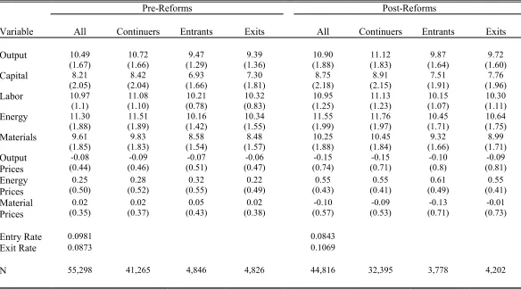
Table 1 presents descriptive statistics of the quantity and price variables just described, for the pre- and post-reform periods, by continuing, entering or ex-iting status. The table reports entry and exit rates of 9.8% and 8.7% during the pre-reform period, but a lower entry rate of 8.4% and a higher exit rate of 10.7% during the post-reform period.9 The quantity variables are expressed in
logs, while the prices are relative to a yearly producer price index to discount inflation. Output increased between the pre- and post-reform periods . Sim-ilarly, except for labor, input use increased between the pre- and post-reform periods. In particular, the table shows that capital, materials and energy use increased between the pre- and post-reform periods especially for incumbents and entrants. On the other hand, labor use decreased between the two periods for entering and exiting plants. Relative prices of output and materials prices declined between the pre- and post-reform periods for all plants.10
8While we observe total employment at the plant-level, we do not observe total hours. Our
method is to impute total hours per worker for plantj using the average for plants in the
same industry as plantj. A large share of the variation in total employment hours stems from
total employment variation.
9These entry and exit rates are lower than those reported for the U.S. and other OECD
countries (Davis, Haltiwanger, and Schuh (1996)). Given that the Colombian economy is
subject to greater rigidities, one may indeed expect lower entry and exit rates in the Colombian context (see, e.g., Tybout (2000) for a discussion of this issue).
10Caution needs to be used in interpreting the aggregate (mean) relative prices in this
context since the relative price at the micro level is the log difference between the plant-level price and the log of the aggregate PPI. On an an appropriately output weighted basis, the mean of this relative price measure should be close to zero in all periods (or one in levels) since the PPI is dominated by manufacturing industries. The larger difference with respect to PPI
in the post-reform period reflects that the growth of manufacturing prices fell more rapidly
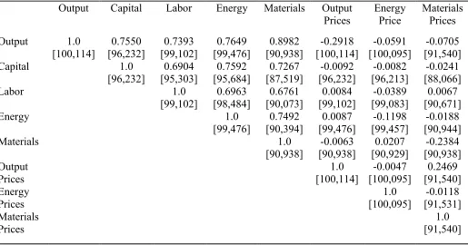
Table 2 reports simple correlations of the various variables reported in Table 1, which display by and large the expected patterns. Output is positively cor-related with all inputs , negatively corcor-related with its own price, and negatively but weakly correlated with energy and materials prices. Inputs are positively correlated with each other. All inputs are negatively correlated with energy prices, except for materials. All inputs are negatively correlated with materi-als prices, except for labor. Energy and materimateri-als use are negatively correlated with their own prices. Also, as expected, output prices are positively correlated with materials prices, and negatively but weakly correlated with energy prices. Finally, energy and materials prices are weakly and negatively correlated.
In the next section, we use these variables to estimate the production func-tion and inverse-demand equafunc-tion.
4
Estimation of TFP and Demand Shocks
We estimate total factor productivity with plant-level physical output data, using downstream demand to instrument inputs. In turn, we estimate demand shocks and mark-ups with plant-level price data, using TFP to instrument for output in the inverse-demand equation.
4.1
TFP Estimation
We estimate total factor productivity for each establishment as the residual from a capital-labor-energy-materials (KLEM) production function:
Yjt=KjtαLβjtE γ jtM
φ jtVjt,
where,Yjtis output,Kjtis capital,Ljtis total employment hours,Ejtis energy
consumption,Mjtare materials, andVjt is a productivity shock. We estimate
this production function in logs,
logYjt=αlogKjt+βlogLjt+γlogEjt+φlogMjt+ logVjt,
so that our total factor productivity measure is estimated as:
T F Pjt= logYjt−bαlogKjt−βblogLjt−bγlogEjt−bφlogMjt. (1)
We deal with this omitted variable bias by using demand-shift instruments which are correlated with input use but uncorrelated with productivity shocks. In particular, we construct Shea (1993) and Syverson (2003) type instruments by selecting industries whose outputfluctuations are likely to function as ap-proximately exogenous demand shocks for other industries. The instruments are total output measures in downstream industries, or combinations of down-stream industries, that satisfy two conditions: (1) they buy a large enough fraction of the output generated by the upstream industry (i.e., the relevance condition), and (2) their purchases from the output industry are a relatively small share of their costs (i.e., the exogeneity condition). The latter condition is important to ensure that the upstream industry is not affecting the down-stream industry, so that the instrument - downdown-stream demand - is uncorrelated with productivity shocks upstream. Thefirst condition is important to ensure relevance of the instruments, i.e., strong correlations between the instruments and use of inputs upstream. Following Shea (1993), we use the input-output matrix for each year to construct instruments for the equivalent of two-digit industries in the U.S.11 For the instruments to meet the two criteria above, we
impose that: (1) the demand share of the downstream industry for upstream production has to exceed 15%, and (2) the cost share of the upstream industry products in the downstream’s total costs is less than 15 percent.12 We also use
one- and two-period lags of the demand shifters. The rationale for doing this is that some factors, such as capital and labor, may face non-linear adjustment costs and irreversibilities, so that demand shifts may take various periods to affect factor utilization. In addition, we use regional government expenditures, excluding government investment, in the region where the plant is located as an instrument to capture shifts in local demand.13 We regard this instrument as
11We use input-output matrices from the national accounts for the pre-1994 period. For the
later years, a new methodology was put in place for the national accounts, and input-output matrices were replaced by output-use and output-supply matrices. For these later years, we rely on output-use matrices to determine cost and sales shares, and on output-supply matrices to determine sectoral output. It is also important to note that input-output matrices do not use ISIC codes to classify industries. The level at which we could create concordance is close to the 2-digits ISIC codes.
12While Shea (1997) uses a criterion of exogeneity based on the ratio of demand share to
cost share (i.e., this ratio being less than 3), our criterion is based on absolute cost shares (i.e., having a cost share of less than 15%). This absolute criterion is more binding than the ratio criterion for downstream industries that represent large demand shares, and less binding for other dowsntream industries. Using the above criteria, adding exports to the downstream demand set and also aggregrating downstream industries to two or three industries to meet the greater than 15% threshold, we obtain instruments for 8 of the 12 upstream industries (i.e., Drinks and Beverages, Wood, Food, Textiles, Oil, Paper, Chemicals and Rubber, and Glass and other non-metallic products). The 4 sectors without demand-shift instruments are Tobacco, which makes up a very low share of sales for other industries; Metals and Machinery, which comprise too high a share of costs when the sales share is high enough; and Other Manufacturing, a category that includes widely different and changing types of goods, for which costs and sales shares are difficult to define in a meaningful a consistent way.
13There may be a common component in technology shocks, although given the enormous
heterogeneity across plants the idiosyncratic component dominates. However, this common
particularly relevant to identify the coefficient on labor, given that labor markets in Colombia are largely region-specific. Finally, we use energy and materials prices as instruments, which are negatively correlated to energy consumption and use of materials, but likely to be uncorrelated with productivity shocks.
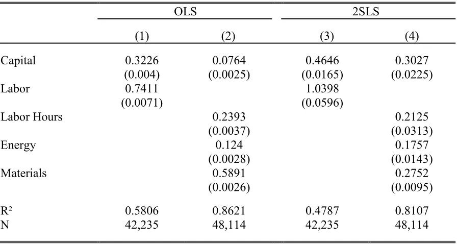
Table 3 reports results for the value-added specification with only capital and employment and for the KLEM specification of the production function. Column (1) reports the OLS results from the estimation of the value-added specification. The results show an elasticity for capital of about 0.3 and an elasticity for employment of about 0.74, which are in line with other studies. The problem with this specification in terms of estimating total factor pro-ductivity is, however, that it imposes implausible restrictions in terms of the elasticity of output to energy and materials. For this reason, we estimate a KLEM specification which uses physical output in the left-hand side and also includes energy and materials as inputs. Furthermore, the inclusion of energy can help account for different levels of capital utilization, under the plausible as-sumption that the latter is positively correlated with the use of energy. Column (2) presents the OLS results from the estimation of the KLEM specification.14
As expected, factor elasticities for capital and labor become smaller, as energy and materials are allowed to impact output in a nonlinear fashion. The results now suggest elasticities for capital, labor, energy, and materials of about 0.08, 0.24, 0.12, and 0.59, respectively.
However, as pointed out above, these elasticities are likely to be biased if productivity shocks are correlated with input use. Columns (3) and (4) of Table 3 present results using 2SLS estimation, which rely on the current and lagged demand-shift instrument, regional government expenditures, and input prices. Even if we think these instruments are weakly correlated with pro-ductivity shocks, large biases could be introduced when using IV estimation if instruments are weakly correlated with the inputs.15 To check whether inputs
economy. Moreover, although certain types of government expenses can constitute
aggre-gate productivity shocks (e.g., construction of road ways), these are likely to show up in the
investment side of the government accounts. This is the reason why we use regional
gov-ernment expenditures, excluding govgov-ernment investment, as an instrument. It is also worth emphasizing that results in the remainder of the paper are robust changing this instrument to total regional government expenditure (which includes government investment), and even to state GDP. That is, we obtain virtually the same results for the estimation of the production functions and all the results that depend upon our TFP and demand shock estimates. Most results are also robust to the exclusion of this instrument but, as we expected, the coefficient of labor hours is very imprecisely estimated in this case, and even has the wrong sign.
14The increase in the number of observations from Column (1) to Column (2) (and also
from Column (3) to Column (4)) is due the fact that Column (1) uses the log of value-added while Column (2) uses the log of physical output as the dependent variable. Observations are lost in the value added specification because the level of value added takes negative values in some cases.
15We also considered longer lags and exponential terms of the demand-shifters as well as
other measures of regional shocks, including total regional government expernditures and state GDP. The results reported here are largely robust to these changes in the list of instruments. To select our baseline instruments, we tested for overidentifying restrictions using a variant of Basmann’s (1960) test, where we estimate a regression of the production function residual
are highly and significantly correlated with the instruments, Table 4 reports results for thefirst-stages of the inputs on the various instruments. The results suggest use of energy and materials increases significantly with downstream de-mand, but employment hours decrease significantly with downstream demand. Moreover, capital, energy use and materials are negatively and significantly correlated with the one-period lag of downstream demand, and all inputs are positively and significantly correlated with the two-period lag of downstream de-mand. Regional government expenditures are positively and strongly correlated with capital and labor and negatively correlated with materials and energy con-sumption. Also, as expected, materials and energy prices significantly reduce energy consumption and use of materials and capital, respectively. Given that we are considering instrument relevance with multiple endogenous regressors, we report the partialR2 measures suggested by Shea (1997) for thefirst-stages, which capture the correlation between an endogenous regressor and the instru-ments after taking away the correlation between that particular regressor with all other endogenous regressors.16 The partial R2’s for capital, employment
hours, energy, and materials in the KLEM specification are 0.1276, 0.139, 0.231, and 0.324, respectively, and 0.2563 and 0.1324 for capital and employment in the value-added specification, showing that the relevant instruments for each input can explain a substantial fraction of the variation in the use of that input. The IV results for the value-added specification in Column (3) of Table 3 show larger capital and employment elasticities relative to the OLS estimated elasticities. The results in Column (4) of Table 3 also show larger elasticities for capital and energy, but smaller elasticities for labor hours and materials, when inputs are instrumented.17 The results from the value-added and KLEM
specifications, thus, indicate that productivity shocks during the period of study are positively correlated with hours and materials and negatively correlated with capital, employment and energy, suggesting the adoption of hour-intensive and energy-saving technologies in Colombia during the 1980’s and 1990’s.
demand shifters turn out to be significant in these regressions, the rest of our instruments
are individually and jointly insignificant. We restrict our instrument list to include those
instruments which are not jointly significant in this regression. Although regional government expenditures (excluding government investment), total regional government expenditures, and state GDP all turn out to be insignificant in this regressions, we rely on regional government expenditures (excluding investment) for the reasons pointed out in Footnote 13.
16The standardR2simply reports the square of the sample correlation coefficient between
Ijtand ˆIjt, whereI=K, L, E, Mand ˆIjtare the predicted values of the inputs from a
regres-sion ofIjt on the instruments. The partialR2 reports the square of the sample correlation
coefficient betweengjt andbgjt, wheregjtare the residuals from an OLS regression ofIjt on all other inputsI1jtandbgjtare the residuals from an OLS regression of ˆIjton the predicted values of all other inputs ˆI1jt.
17The value-added specification ignores changes in labor utilization. If technology shocks
are negatively correlated with employment but positively correlated with labor hours, this
would explain why the elasticity of labor increases when the value-added specification is
in-strumented, while the elasticity of labor hours falls when the KLEM specification is
4.2
Estimation of Demand Shocks
While productivity is likely one of the crucial components of profitability, other components of profitability are also probably important determinants of reallo-cation. For example, even if plants are highly productive, they may be forced to reduce their market shares if faced with large negative demand shocks. We cap-ture the demand component of profitability by estimating establishment-level demand shocks as the residual of the following inverse-demand equation:18
Pjt=Yjt−εDjt,
whereDjtis a demand shock faced byfirmjat timetand−εis the inverse of the
elasticity of demand and 1+εis the mark-up. We estimate this inverse-demand function in logs,
logPjt=−εlogYjt+ logDjt,
and our demand shock measure is estimated as the residual from this regression,
djt=logdDjt= logPjt+bεlogYjt, (2)
where −bε is an inverse measure of the elasticity of demand. Using OLS to estimate the inverse-demand function is likely to generate an upwardly biased estimate of demand elasticities because demand shocks are positively correlated to both output and prices, so thatbεwill be smaller in absolute value than the trueε. To eliminate the upward bias in our estimates of demand elasticities, we propose using TFP as an instrument forYjt since TFP is positively correlated
with output (by construction) but unlikely to be correlated with demand shocks. Table 5 reports the results of the inverse-demand equations using both OLS and IV estimation. Columns (1)-(3) present OLS results of inverse-demand equations, some of which impose the same elasticity while others allow different elasticities for the pre- and post-reform periods. Columns (4)-(6) present equiv-alent 2SLS results.19 Column (1), which presents OLS results when imposing
the same elasticity before and after the reforms, suggests a large elasticity of 11.05 for the entire period of study. The results in Column (2) which allow for different elasticities before and after the reforms suggest demand elasticities of 11.66 and 10.94 during the pre- and post-reform periods, respectively.20 By contrast, the results in Column (3), which allow for different intercepts and dif-ferent elasticities after the reforms, show elasticities of 22.37 and 7.37 during
18There are other important components of profitability that we do not measure, such as
access to credit markets.
19The sample size is larger in this table than in Table 3 because the estimations in Table
3 require information on the instruments used for estimating the production function, while demand estimations only require information on output prices, physical output, and TFP estimates.
20The pre-reform elasticity is calculted as the inverse of the estimated physical output
the pre- and post-reform periods, but higher demand after the reforms. As indicated, however, caution needs to be exercised in interpreting these as elas-ticities since these coefficients capture the fact that higher demand implies a positive correlation between output and prices.
The 2SLS results, which use TFP as an instrument for output, indeed show much lower elasticities.21 The results in Column (4) show a demand elasticity
of 2.28, while the results in Column (5) show a demand elasticity of 2.24 during the pre-reform period and of 2.3 during the post-reform period. By contrast, allowing for different intercepts and elasticities before and after the reforms suggests elasticities of 3.17 before the reforms and of 1.88 after the reforms, but higher demand after the reforms at given price levels.22The last three columns
in Table 5 report high total and partialR2’s.23 The partial R2’s for physical
output and physical output interacted with the post-reform dummy on TFP, a post-reform dummy, and TFP interacted with the post-reform dummy are of 0.427 and 0.4621, indicating relevance of the instruments. These results suggest quantities responded less to changes in prices but overall demand was higher after the reforms. Increased demand after reforms may be explained by scale effects generated by trade liberalization measures and by the downward shift in average production costs induced by factor market reforms.
5
TFP, Demand, and Prices Before and After
the Reforms
In this section we rely on the TFP and demand shock measures estimated in the last two sections as well as on output prices to document differences in the productivity and demand components of profitability in Colombia during the 1980’s and 1990’s in terms of heterogeneity and persistence. We are, for
21The negative R-squares for the 2SLS are not surprising and should not be viewed as
alarming. Output and the demand shocks are highly positively correlated (this is the entire
reason for using 2SLS rather than OLS). Using the simple inverse-demand equation, the
variance of prices will be equal to terms involving the variance of output, the variance of demand shocks and a term that depends negatively on the covariance of output and demand shocks (given that the demand elasticity is negative). Thus, the variance of demand shocks will exceed the variance of prices and, hence, the negative R-squares.
22Robustness analysis suggests that while it is important to use a TFP measure as an
instrument in the demand equations for output (i.e., elasticities are quite different between OLS and 2SLS in demand equation), it matters much less whether the TFP used is from OLS or 2SLS estimation of production equation. This reduces concerns about sensitivity of
results to instrument selection for production equations. In addition, we considered energy
and materials prices as instruments for physical output in the inverse-demand equations and
wefind that the results are very similar whether we use TFP alone or TFP and energy and
materials prices as instruments.
23The totalR2 simply reports the square of the sample correlation coefficient betweenY
jt andYbjt, whereYbjtis the predicted value of output from a regression ofYjton the instruments. The partialR2 reports the square of the sample correlation coefficient betweenujtandubjt, whereujtare the residuals from an OLS regressions ofYjtonYjt×P ost−ref ormandbujt
are the residuals from an OLS regression of the predicted value ofYjton the predicted value
example, interested in documenting whether productivity is as heterogeneous and persistent in Colombia as it is in other countries.
Before turning to these issues, however, we report in Table 6 basic descrip-tive statistics of TFP, demand shocks and output prices for the periods before and after the reforms. The table shows an increase in the simple means of total factor productivity and our demand shock measure, but a decrease in the mean of output prices. Caution needs to be used in interpreting these simple averages. For TFP, as we emphasize later aggregate TFP can be decomposed into a term based upon the simple (unweighted) average and a covariance term reflecting the relationship between market share and TFP. The latter can be interpreted as an index of the efficiency of the allocation of resources and as we show later is very important in Colombia. With respect to relative prices and demand shocks, note that the average price is the average price of plant output relative to the PPI. The average demand shock is the average of the demand shocks constructed from a micro model of relative prices across plants. On the other hand, the table shows a substantial increase in the dispersion of TFP, demand shocks, and output prices. The standard deviations of TFP, demand shocks and prices increased from 0.68 to 0.91, from 0.78 to 0.88, and from 0.44 to 0.74, respectively. In addition, as expected, Table 6 shows a negative corre-lation between prices and TFP and output, and a positive correcorre-lation between demand shocks and prices both before and after the reforms, though the corre-lations are stronger after the reforms. By contrast, TFP and demand shocks are positively correlated during the pre-reform period but negatively correlated after the reforms. This correlation points to the effects of trade reform: after trade liberalization, producers in sectors most exposed to import competition will simultaneously increase productivity and lose demand. In contrast, man-ufacturers in sectors least exposed to import competition will have relatively less incentives for productivity enhancement and will less likely face a drop in demand. In addition, the table shows that firms facing higher demand and productivity shocks produce more output, both before and after reforms. How-ever, while the relation between output and productivity becomes stronger after the reforms, the relation between output and demand becomes weaker. This correlation suggests, again, that the reforms were successful in strengthening the link between a business’s performance and its productivity. Moreover, this table shows that not only do more productive firms increase production after the reforms, but they also increase their share in the market. This points to the increased importance of productivity-enhancing reallocation after the reforms, which we document in Section 6.
5.1
Heterogeneity
Colom-bian plants. Figures 1-3 show the evolution of dispersion measures of TFP, demand shocks and output prices over the entire period of study.24 The fi
g-ures show large percentage increases in the dispersion of productivity and prices over the last two decades. In particular,figures 1 and 3 shows large rises in the dispersion of productivity and prices of entering and exiting plants after 1990, and a constant increase in the dispersion of productivity and output prices of continuing plants throughout the entire period. By contrast, Figure 2 shows a much smaller percentage increase in the dispersion of demand over the last two decades. The greater heterogeneity in productivity is consistent with greater process experimentation across businesses after reforms, while the modest in-crease in the dispersion of demand is consistent inin-creased competition, and also with modest increased experimentation in product variety across businesses.
Figures 4-6 show Kernel distributions of TFP, demand shocks and output prices for the pre- and post-reforms periods, which illustrate changes in higher moments of the distributions. The distributions display fatter tails (i.e., in-creased kurtosis) of the distributions of TFP, demand shocks and output prices after the reforms, suggesting that morefirms were experiencing either positive or negative large shocks after the reforms.
5.2
Persistence
To examine whether Colombian plants, like U.S. plants, are characterized by a large degree of persistence, we estimate AR(1) models for productivity, demand shocks and prices. Columns (1), (3) and (5) in Table 7 report the coefficients on the lags of productivity, demand and output prices for AR(1) models with year effects. Our estimates show a great deal of persistence of productivity, demand shocks and prices in Colombia , much greater than that found for the U.S. The results suggest that 67% of all plants continue with their initial productivity after 5 years, 93% of plants face the same demand shocks after 5 years, and 96% charge the same prices as 5 years ago. Studies for the U.S. find much lower degrees of persistence. For example, Bartelsman and Dhrymes (1998)
find that after 5 years only about a third of all plants remain in the same productivity quintile. Foster, Haltiwanger and Syverson (2003) also find that about a third of plants remain in their original position in the productivity and price distributions after 5 years. In spite of the reforms increased competition after the reforms, the greater persistence in the Colombian context probably reflects continued presence of distortions in this economy.
Columns (2), (4), and (6) in Table 7 also report how the degree of per-sistence changes after the market reforms. The results suggest persistence in productivity and output prices increased after the reforms, while the persistence of demand shocks did not change. Atfirst glance, this pattern might be surpris-ing as one might conjecture that market reforms would lead to greater mobility in the distributions of efficiency, demand shocks, and prices. However, it is
24We have examined these patterns using alternative robust measures of dispersion (in
important to emphasize that these persistence measures are conditional on sur-vival. Our results are consistent with increased weeding out of less productive plants, as reported in the next section, but lower mobility of the plants that do survive after the reforms.
6
Productivity- and Pro
fi
tability-Enhancing
Re-allocation
In this section, we examine whether the market reforms changed the alloca-tion of activity in terms of productivity and demand factors. In particular, we are interested in whether increased competition as a result of the reform process induced reallocation from less to more productive plants and reduced the role of demand factors in the allocation of activity. Similarly, we are in-terested in whether increased competition as a result of the reforms increased productivity by making it more difficult for less productive plants to enter the market and survive. Different types of models have been proposed which can explain productivity-enhancing reallocation of this sort. In learning models (e.g., Jovanovic (1982), and Ericson and Pakes (1989)), experimentation gener-ates differences in productivity and successful experimenters gain market share over unsuccessful ones. Similarly, vintage capital models can explain gains in market share of plants with newer vintages over those with older vintages. If more efficient plants can afford more frequent retooling, initial productivity differences would be exacerbated. Moreover, if trade liberalization and FDI increased competition in product markets after the reform process, this may have speeded up learning and productivity-enhancing reallocation. Similarly, if
financial liberalization in 1992 improved access to credit markets, this may have provided access to better capital vintages and increased productivity-enhancing reallocation after the reforms.
6.1
Productivity Growth and Reallocation
We use a cross-sectional decomposition methodology,first introduced by Olley and Pakes (1996), to examine whether the allocation of activity in the economy has become more or less productivity-enhancing over our period of study. We conduct the following decomposition of aggregate TFP and total demand shocks, constructed from our estimates of plant-level TFP and demand:
T F Pt = T F Pt+ J
X
j=1
¡
fjt−ft¢ ¡T F Pjt−T F Pt¢,
dt = dt+
J
X
j=1
¡
fjt−ft
¢ ¡
djt−dt
¢
whereT F Ptand dt are aggregate total factor productivity and demand shock
measures for a given 3-digit manufacturing sector in year t. These aggregate measures correspond to weighted averages of our plant-level measures TFP and demand shocks, where the weights are market shares (calculated as described below). T F Ptanddtare the cross-sectional (unweighted) means of total factor
productivity and demand shock measures across all plants in that sector in yeart,T F Pjtanddjtare total factor productivity and demand shock measures
of plant j at time t estimated as described in Section 4, fjt is the share or
fraction of plantj0soutput out of sectoral output at the 3-digit level in yeart,
andftis the cross-sectional unweighted mean offjt.25 The second term in this
decomposition allows us to understand whether production is disproportionately located at high-productivity or high-demand plants. Moreover, by examining this decomposition over time we can learn whether the cross-sectional allocation of activity has changed in response to the market reforms.26
Table 8 shows the cross-sectional decompositions for TFP and demand shock measures from 1982 to 1998. We report the results for the average 3-digit sector. Column (1) shows a positive trend in aggregate total factor productivity over the period of study. Columns (2) and (3) show the decomposition of aggregate productivity into the simple average and the cross-sectional correlation between market share and total factor productivity. In all years, aggregate productivity is largely accounted for by the allocation of activity to higher productivity businesses, as shown by the large fraction that the cross-term represents out of aggregate productivity. This stands in sharp contrast to results of similar exercises for the U.S., where the contribution of this term is only marginal (see Foster, Haltiwanger and Krizan (2001)). In a context in which the production possibilities frontier is not improving sharply over time, the allocation of activity seems to be the crucial factor accounting for the level of aggregate productivity. The cross-sectional correlation between market share and total factor pro-ductivity remained roughly constant over the 1980’s, with a slight decrease by the middle of the decade. By contrast, it increased sharply during the 1990’s, most specially after 1993, once most reforms were fully implemented. This time-series pattern can be seen in Figure 7 and suggests that market share increasingly shifted towards more productive plants and away from less produc-tive plants during the 1990’s. In fact, while average productivity explains about
25This means that our focus here is on within sector allocation and reallocation rather
than between sector allocation, for sectors defined at the 3-digit level. For measurement and
conceptual reasons, comparisons of TFP and relative demand across sectors (in levels) are more problematic to interpret. Focusing on within sector allocation permits us to emphasize the degree to which market reforms have led to an improved allocation of activity across businesses due to higher competition. Nevertheless, we have also tried a decomposition using the shares or fraction of plant output out of total output. The results based on this alternative decomposition are similar to those reported below.
26An advantge of this cross-sectional method over methods that decompose changes in
productivity over time, is that cross-sectional differences in productivity are more persistent
and less dominated by measurement error or transitory shocks. Another advantage is that
8.6% of aggregate productivity during the pre-reform period, it only explains about 5.5% of aggregate productivity during the post-reform period.
Columns (1)-(3) in Table 9 provide evidence of the statistical significance of the effects of reforms on the Olley-Pakes decomposition of TFP, just described. Each of these columns reports results of regressing one of the terms of the TFP decomposition on a post-reform dummy that takes a value of 1 in 1991-1998, and ISIC 3-digit sector controls, using data at the 3-digit level. Column (1) shows results using aggregate TFP (the weighted average of TFP using market shares as weights) as dependent variable. The results show a statistically significant increase in aggregate TFP after the reforms. Column (2) reports results of a regression of the simple average of TFP. These results show no significant change in the unweighted mean of TFP. Finally, column (3) reports results of a regression of the cross-sectional correlation between market share and TFP. The results show a significant increase of almost 50% (with respect to the magnitudes reported in Table 8) in the correlation between market share and TFP after the reforms. Thus, the post-reform period is characterized by a significant increase in the ability of highly productivefirms to gain market share.27
The last three columns of Table 8 show the Olley-Pakes decomposition of our demand shock measure, since we are also interested in whether the reform process changed the role of demand factors in the allocation of activity. Column (4) shows a decreasing trend of aggregate demand shocks over the period of study, although the average plant actually perceived an increase in demand (column (5)). Moreover, in contrast to the results on productivity, Column (6) suggests that the concentration of activity in high demand plants became less important during the 1990’s. Figure 8 shows the time-series pattern of this decomposition.
The statistical significance of the effects of reforms on the decomposition of demand shocks is analyzed in columns (4)-(6) of Table 9. As was the case for the decomposition of TFP, each of these columns presents the results of a regression of one of the components of the decomposition of demand on the post-reform dummy and sector controls, using data at the 3-digit sector level. The dependent variable in column (4) is the aggregate demand shock, in column (5) it is the simple average of plant-level demand shocks, and in column (6) it is the cross term of the decomposition. The results indicate a negative and statistically significant change in aggregate demand shocks after the reforms (column (4)), although the magnitude of the change is small relative to the magnitudes of aggregate demand shocks, as reported in Table 8. Nevertheless, the demand shocks faced by the average plant experience a positive and significant change with the reforms. The decline in aggregate demand shocks is explained by a decrease in the correlation between demand shocks and market share, which fell significantly after the reforms. These effects point to a decline in the relative importance of high demand in gaining market share.
27As reform does not significantly change the simple average of TFP, rather than plant
Our results suggest that the packet of reforms, most likely through its com-ponents of trade liberalization, removal of FDI restrictions and liberalization of factor markets, contributed to raise productivity by improving the allocation of activity with higher market shares at high-productivity plants and lower mar-ket shares at low-productivity plants. At the same time, we find that, after the reforms, the allocation of activity was driven less by high demand plants commanding larger shares. This latter finding is consistent with the hypoth-esis that increased competition reduced the influence of demand factors (i.e., markets became more competitive) in the allocation of activity.
6.2
Entry and Exit E
ff
ects
Vintage capital models of industry dynamics suggest new firms are relatively more productive, as they receive the productivity associated with the latest vintage technology, and once they have entered the market their productivity remains constant over time unless hit by random shocks. Then, firms exit the market when the productivity relative to new entrants is below a certain threshold. However, aside from Foster, Haltiwanger and Syverson (2003) who
find higher productivity of entering plants and lower productivity of exiting plants, the previous literature documents lower productivity of both entering and exiting relative to incumbent plants (see Bartelsman and Doms (2000)), a
finding that is at odds with the vintage capital model. Uing our estimates of TFP and demand shocks, we analyze this issue for the Colombian economy, and explore whether the market-oriented reforms changed how productive entering and exiting businesses are relative to incumbents.
Table 10 reports regressions of TFP, demand shocks, and prices on year dummies as well as on entry and exit dummies. The entry dummy takes a value of 1 for plantj in periodtif the plant produced in yeartbut not int−1 . Conversely, the exit dummy takes a value of 1 for plantj in periodt if plant
j produced in periodt but not int+ 1. Column (1) in Table 10 shows that , consistent with the vintage capital hypothesis, productivity of entering plants is above and productivity of exiting plants below that of the average incumbent. Our results coincide with those in Foster, Haltiwanger, and Syverson (2003). Like theirs, our TFP estimation uses physical output rather than revenue, which avoids confounding price and productivity variations in measures of TFP. The results in Column (5) also show lower idiosyncratic demand for entering and exiting plants relative to the average incumbent, and the results in Column (9) show entrants and exiting plants charging higher prices than incumbents. While higher prices at exiting plants are consistent with their lower productivity, higher prices at entering plants might reflect their smaller scale or perhaps higher markups.
results in Column (2) of Table 10 show a much smaller differential entry effect on productivity after the reforms. That is, after the reforms, entering busi-nesses had a smaller productivity advantage relative to incumbents in the year of entry. Lower adjustment costs due to less distorted factor markets appear to show a greater ability of surviving incumbents to catch-up with potentially highly productive entrants. First, they can retool more frequently to install latest vintage technologies. Second, this is consistent with increased layoffs of unproductive workers after the reduction in dismissal costs in 1990. Alterna-tively, there may have been increased market experimentation after the reforms so that the average entrant had lower initial productivity. This latter idea we explore further below.
On the other hand, the results suggest that productivity of exiting plants relative to incumbents fell substantially after the reforms. This pattern is consistent with increased exit of plants which may had been kept afloat by subsidized credit, relatively low taxes, and lack of international competition before 1990. On net, the contribution of entry and exit to overall productivity rises slightly after the reforms. Moreover, the results show that relative demand for entering and exiting plants did not change after the reforms. On the other hand, relative prices of both entering and exiting plants increased after the reforms.
We also examine learning effects by looking at the evolution of productivity, demand, and prices of plants over thefirst years they are in the market. The results in Column (3) of Table 10 , for the entire period, include one- and two-period lags of the entry dummies and one- and two-two-period leads of exit dummies, capturing plants that entered int−1 andt−2 and plants that will exit int+ 1 andt+2. The results show little evidence of learning prior to market reforms, as businesses do not appear to be more productive one or two years after entering than they were upon entrance. However, after market reforms there is evidence of substantial learning amongst entrants. As noted, the productivity advantage of entrants diminished after reforms but the productivity advantage two years after entry increased after the reform. This pattern is consistent with the hypothesis mentioned above of increased market experimentation by entrants after the reforms.
We also examine a number of other patterns in terms of entry and exit. It is interesting to note that there is evidence of a “shadow of death” effect: the negative productivity differential faced by exiting plants becomes stronger the closer to exiting the plant is. This effect grows stronger after reforms. We alsofind some evidence of ”learning” in terms of demand and prices. In this context, we mean that entering plants appear to gain a greater demand/price advantage as time after entry grows. Column (7) and (11) show that , as time elapses since plant entry, the plant’s relative demand grows and the prices it charges for the output fall. Columns (8) and (12) show greater learning effects in demand and prices after the reforms.
financial reforms may have previously encouraged entry of unproductive plants and kept existing unproductive plants afloat. Moreover, greater learning after reforms may be due to greater access to new vintages of imported capital and greater access to the know-how of foreignfirms in the economy. In terms of exiting behavior, intensified foreign competition after the trade reforms seems to have increased market discipline by forcingfirms either to increase productivity and charge lower prices, or else exit the market.
7
Conclusion
In this paper, we examine how reallocation contributes to productivity and other determinants of profitability in Colombia. Then, we ask how the relation between reallocation and productivity and demand factors changed after market reforms were introduced in Colombia during the early 1990’s. The extent, breadth and swiftness of the reforms make Colombia a superb country to study these issues. In addition, a unique feature of the Colombian data is that it allows us to measure both plant-level quantities and prices, making these data ideal for measuring plant-level productivity and demand.
We propose a sequential methodology for estimating both productivity and demand shocks at the plant level. First, we generate measures of plant-level total factor productivity by estimating KLEM production functions using plant-level physical output data. To eliminate biases from the correlation between productivity shocks and inputs, we use downstream demand shifts and plant-level energy and materials prices as instruments in estimating production func-tions. We then generate plant-level demand shocks by estimating inverse-demand equations using plant-level output prices, where output is instrumented with TFP to eliminate biases from the correlation between demand shocks and output.
We find some interesting patterns with regards to total factor productiv-ity, prices and demand shocks in Colombia, which sometimes contrast with the patterns found for the U.S. First, as in the U.S., wefind a great deal of het-erogeneity in terms of productivity and output prices, and we find that this heterogeneity has been increasing over the past decades. Second, we find a large degree of persistence in productivity, prices and demand, which doubles or triples the degree of persistence found in the U.S.