See discussions, stats, and author profiles for this publication at: https://www.researchgate.net/publication/265065031
SEISMIC ANALYSIS OF SPHERICAL TANKS
INCLUDING FLUID-STRUCTURE-SOIL
INTERACTION
Article
CITATIONS
0
READS
33
3 authors:
Some of the authors of this publication are also working on these related projects:
Novel demountable shear connector for accelerated disassembly, repair or replacement of
precast steel-concrete composite bridges
View project
Innovative seismic-resistant steel frame with high post-yield stiffness dampers for drift
reduction
View project
Theodore L. Karavasilis
University of Southampton
45PUBLICATIONS 392CITATIONS
SEE PROFILE
Dimitris C. Rizos
University of South Carolina
44PUBLICATIONS 341CITATIONS
SEE PROFILE
Dimitris L. Karabalis
University of Patras
57PUBLICATIONS 830CITATIONS
SEE PROFILE
All in-text references underlined in blue are linked to publications on ResearchGate, letting you access and read them immediately.
13
thWorld Conference on Earthquake Engineering
Vancouver, B.C., Canada August 1-6, 2004 Paper No. 1814
SEISMIC ANALYSIS OF SPHERICAL TANKS
INCLUDING FLUID-STRUCTURE-SOIL INTERACTION
T.L. Karavasilis
1, D.C. Rizos
2, and D.L. Karabalis
1SUMMARY
The accurate and efficient, from a practical point of view, analysis of spherical tanks is the primary motivation for this work. The proposed methodology implements: (a) the Boundary Element Method (BEM) for the simulation of the soil-structure interaction, (b) a discrete 2-DOF mechanical system for the approximate computation of the impedances of a massive, rigid, ring foundation, a usual feature of a spherical tank, and (c) a FEM simulation of the structure and fluid regions. The above modules are coupled via the pre- and post-processing capabilities of the widely used general purpose program ANSYS. The entire analysis is performed directly in time domain assuming linear elastic structure and soil region.
INTRODUCTION
Mechanical systems consisting of structures, fluid, and soil regions are representatives of multi-phase systems. The comprehensive and accurate analysis of multi-phase structural systems in dynamic environments has substantial impact in the structural design procedures, especially whenever relative motion among the phases is expected. Such cases can be classified into problems with large relative motion governed by flow characteristics, problems of short duration, and problems of long duration with limited fluid displacement. The latter includes such typical Fluid-Structure-Soil-Interaction (FSSI) phenomena as the dynamic response of offshore structures, nuclear reactor components, liquid filled tanks, and dams subjected to waves or earthquakes. Information pertaining to the developments in the fields of dynamic interaction problems can also be found in the review articles, and references therein, of Rizos and Karabalis [13], Beskos [2,3], and Mackerle [8], among others.
The analysis of spherical tanks is the primary motivation for this work. To this end, the main emphasis lies on a practical, yet “accurate”, procedure to simulate the soil-foundation interaction while taking into consideration, through standard FEM procedures, the fluid-structure interaction. The proposed methodology implements: (a) the Boundary Element Method (BEM) for the simulation of the
1
Department of Civil Engineering, University of Patras, 26500 Patras, GREECE
structure interaction, (b) a discrete 2-DOF mechanical system for the computation of the impedances of a ring foundation, a usual feature of a spherical tank, and (c) a FEM simulation of the structure and fluid regions. The above modules are coupled via the pre- and post-processing capabilities of the widely used general purpose program ANSYS. The entire analysis is performed directly in time domain assuming linear elastic structure and soil region. However, taking into account nonlinear behavior, both material and geometric, of the structure is a straightforward matter within the framework of the proposed procedures.
The FEM methods are well-established procedures (e.g. [1,15]). These methods routinely accommodate complex geometries and non-linear phenomena. The matrices associated to the algebraic system of equations are symmetric, banded and positive definite, allowing the implementation of efficient solution algorithms. The nature of the FEM implies that the solution domain must be finite. However, cases involving infinite media, such as the soil region, cannot be represented according to classical FEM procedures. The treatment of the radiation condition, imposed by the infinite extent of the soil medium, has lead to the development of numerous special types of radiating, transmitting or absorbing elements for use predominantly in the frequency domain FE method, e.g. Rizos and Karabalis [13].
Boundary Element Methods for SSI analysis are based on integral formulations and fundamental solutions of the wave propagation problem. Such formulations satisfy implicitly the radiation boundary condition of infinite domains, and are appealing alternatives to the FEM. They require discretization of the boundary of the solution domain only. Consequently, BEM methods reduce the dimensionality of the problem by one, yielding smaller systems of algebraic equations. However, the matrices associated with the BEM algebraic system of equations are, in general, not symmetric and fully populated. BEM can accommodate nonlinear phenomena, but in this case additional volume discretizations are required. Comprehensive reviews on BEM are reported by Beskos [2,3]. Time domain BEM solutions for 3-D problems associated with the proposed formulation have been presented by Karabalis and Beskos [4, 5, 6, 7], Rizos and Karabalis [11,12], Rizos [10] and Rizos and Loya [14], among others.
SOIL-FOUNDATION INTERACTION BY BEM-FEM
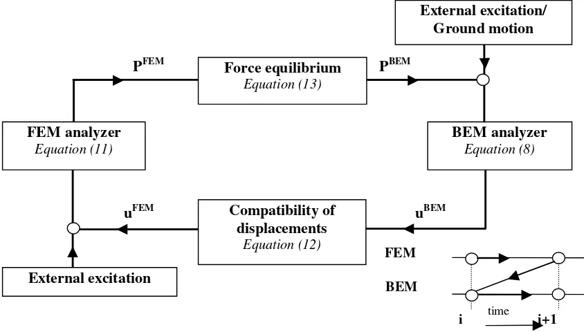
A coupled BEM-FEM methodology suitable for 3-D dynamic SSI analysis and wave propagation is proposed for the simulation of the soil-foundation system. The proposed FEM-BEM is derived in time domain based on the BEM formulations presented by Rizos [9] and Rizos and Karabalis [11,12] and standard FEM analysis procedures for solids and structures. The foundation is modeled by finite elements, while the linear soil region, of semi-infinite extent, is modeled by boundary elements. The BEM method is used to compute the B-spline impulse response of the surface of the BE domain, in general, and of the BE-FE interface, in particular. In contrast to other formulations reported in the literature, the coupling of the two methods is performed in a staggered solution approach in direct time domain. According to this, the solution of one method serves as initial conditions to the other at every time step, as demonstrated in Figure 1. Although the BEM-FEM methodology has been developed for the analysis of flexible structures resting on an elastic half-space, in this work its usefulness is limited to the computation of the response of a rigid ring foundation, which is the usual case in conjunction with spherical tanks.
B-spline BEM Formulation
time dependent variables without excessive computational effort and implicitly satisfy the continuity conditions of the Stokes fundamental solutions. A detailed formulation and integration of the B-spline fundamental solutions and of the associated BEM can be found in the work of Rizos [9], Rizos and Karabalis [11,12], and Rizos and Loya [14]. In the present outline symbols in boldface indicate vectors or tensors, dots indicate differentiation with respect to time and indicial summation notation is adopted where appropriate.
Figure 1. Schematic representation of the proposed BEM-FEM coupling scheme.
Following well-established procedures, the Love integral identity form of the Navier-Cauchy governing equations of motion for a linear isotropic and homogeneous elastodynamic medium can be expressed in a
discrete form, in space and time, at time instant tN, as
( )
t
(
( )
t
( )(
) ( ) (
t
)
)
M
N
M
n
n N n n
N n
N
=
∑
−
≥
= − −
,
1τ
τ
T
u
t
U
cu
n (1)where
1
1 2
1
− + + +
= −+ − + −+ −
−
k
t t
tN n N n N n k
n N
L
τ
The discrete form of Eq. (1) implies that:
(i) B-spline fundamental solutions of the kth order for the infinite elastodynamic space are adopted.
The support of the associated B-spline polynomials is ∆t. The summation indicated in Eq. (1) refers
to discrete time steps, and M depends on the order of the B-spline fundamental solutions. For
example for the cubic B-spline fundamental solutions M=N+2.
(ii) The temporal discretization of the field variables is based on B-spline function approximation
schemes of the same order as the B-spline fundamental solutions. Eq (1) is evaluated at time knot tN
and the associated time knot sequence is
PBEM PFEM
uFEM uBEM
BEM analyzer
Equation (8)
External excitation/ Ground motion
External excitation FEM analyzer
Equation (11)
Compatibility of displacements
Equation (12)
Force equilibrium
Equation (13)
time FEM
BEM
(
)
k
odd
n
N
M
k
t
n
even
k
k
t
n
t
n0
,
1
,
2
,
,
,
,
5
.
0
L
L
=
∆
−
∆
=
(2)where ∆t is the support of the adopted B-spline polynomials.
(iii) The surface S of the elastodynamic domain is discretized in a total of NE surface elements for a
total of NN boundary nodes. The present work implements higher order 3-D surface elements in an
isoparametric formulation.
The tensor cij in Eq. (1) is known as the “jump” term and depends on the location of a discrete node with
respect to the solution domain and its boundary, and the geometric characteristics of the domain in the
neighborhood of the node. The coefficient matrices U(t) and T(t) are of size 3NN x 3NN and represent
the influence of a source boundary node on a receiver boundary node. These matrices are evaluated based on integrals of the B-spline fundamental solutions over the surface of each element for all boundary nodes.
Vectors t(n) and u are of size 3NN x 1 and represent the components of the traction and displacement
fields, respectively, at every boundary node due to a single B-spline impulse excitation applied at time τ.
As reported in Refs [10] and [14], nodal forces, p, can be related to tractions, t(n), through a transformation
matrix L that is developed based on a virtual displacement approach, allowing Eq. (1) to be expressed in
terms of nodal forces, p, as
( )
∑
(
( ) (
) ( ) (
)
)
= − −
−
=
Nn
n N n n
N n
N
t
t
t
1
τ
τ
T
u
p
G
cu
(3)where
G
=
UL
−1 and∑∫
=
=
Aa S
a s T s
a
dS
1
N
N
L
. The integration is over the area, Sa, of each element, thesummation indicates superposition over the number of elements, A, that contain a soil node, and Ns are
the shape functions of the spatial discretization.
The impulse response of the elastodynamic system can be obtain from Eqs (1) or (3). To this end, a
B-spline impulse force, or traction, excitation of duration ∆t is applied in the direction of each degree of
freedom, j. Eqs (1) or (3) are solved in a time marching scheme for the displacements, u, which represent
the B-spline impulse response vector, bNj . These impulse responses can be collected in matrix form as
( )
[
N]
NN N
j N
N N N
t B b1 ,b2 , ,b , b3
B = = K K (4)
The dimension of matrix B(tN) is 3NN x 3NN , in general, and each column,
N j
b , represents the impulse
response of all degrees of freedom at time step tN due to a unit traction, or force, applied at degree of
freedom j. This matrix is a characteristic of the system and needs to be computed only once for the
specific geometry of the free surface of the elastodynamic domain. In the general case, the B-spline impulse response is computed for all degrees of freedom of the problem and the impulse response matrix,
BN, is square. In most practical cases, however, the impulse response of the system needs to be computed
only for those degrees of freedom that are expected to carry forces (contact loads or incident fields) of the arbitrary excitation, yielding a rectangular matrix or a square matrix of significantly reduced size, as shown in Ref. [14].
Once this characteristic response of the system is known, the system can be analyzed for any arbitrary
transient excitation, f(t). Let f(t) represent the vector of arbitrary transient external excitations applied at
the boundary nodes of the elastodynamic system and
f
n=
f
(
t
=
t
n)
the value of the excitations at timestep tn. Furthermore, let RN represent the response of the elastodynamic system to the excitation f(t) at time
step tN. If the B-spline impulse response, BN, matrix of the system is known, the calculation of RN reduces
to a mere superposition of the B-spline impulse responses as
∑
=+ − +=
1 1 2 N n n N n Nf
B
R
(5)This approach is very efficient especially when multiple load cases are considered.
Eq. (5) can be specialized for the proposed coupling scheme. To this end, the vector of arbitrary
excitations
f
=
{ }
P
c,0
T consists of nodal forces Pc, applied at the contact interface between the BE andFE domain only, while the free field is not loaded. The response R of the BEM region pertains to nodal
displacements
u
=
{
u
c,
u
f}
Tdue to the contact forces at time step N. In view of the separation intocontact and free field degrees of freedom, Eq. (5) can be expressed as
∑
+ = + −⇒
=
1 1 2 N n n N c n ff fc cf cc N f c0
P
B
B
B
B
u
u
∑
+ = + −=
1 1 2 N n n N c n cc Nc
B
P
u
(6a)∑
+ = + −=
1 1 2 N n n N c n fc Nf
B
P
u
(6b)It is evident that only that part of the B-spline impulse response matrix that corresponds to the contact degrees of freedom is required. In addition, the response of the free field can be computed independent of that of the contact area. For this reason only Eq. (6a) shall be considered in the proposed coupling
scheme. The interface forces, Pc, however, depend on the response of the FE region and are not known in
advance. Consequently, Eqs (6) are in an implicit form. The corresponding explicit scheme is obtained
by interpolating the interface forces at time tN using B-spline polynomials. For the cubic B-spline
polynomials (k=4) implemented in this work, the interface forces are interpolated as
1 1 1 1 1 4 4 1 4 2 6 1 3 2 6 1 4 1 2 1 4 3 − + + − + − − = ⇒ + + = + + = N c N c N c N c N c N c N c o N c o N c o N
c B B B
P
P
P
P
P
P
P
P
P
P
(7)Introducing Eq. (7) into (6a) and separating known from unknown quantities with respect to time step N,
(
)
N N c N c N c cc N n n N c n cc N c cc cc N cH
FP
u
P
B
P
B
P
B
B
u
+ = ⇒ − + + = + − = + −∑
1 1 13 2 2 1 2 (8)
where
F
=2
B
1cc +B
cc2 represents the flexibility matrix of the contact interface of the BEM region and1 1 1 3 2 − + = + − −
=
∑
Nc cc N n n N c n cc
N
B
P
B
P
H
is a vector representing the influence of the response history on thecurrent step. Eq. (8) is used in the proposed coupling scheme and represents the BEM solver. It is evident that if the contact forces are provided by the FE solver, at every step N, the BE solver evaluates the corresponding displacements of the interface without solving a system of algebraic equations. Furthermore, if the response of the free field is of interest, it can be computed by a simple evaluation of Eq. (6b).
Time Domain FEM Formulation
This section presents an outline of the FE procedures as implemented in the present work in a
manner suitable for coupling with the BEM. The FEM is used to model the structural
component in a soil-structure system subjected to transient excitations. The governing equations
are integrated directly in time using two different time stepping algorithms, i.e. the backward
difference scheme and the Newmark-
β
method.
Governing Equation
The governing equations of motion of a multi-degree of freedom system, as derived in a semi-discrete FE approach, is expressed in matrix form as,
( )
t Cu( )
t Ku( ) ( )
t f t uM&& + & + = (9)
These are second order differential equations with M, C, and K being the mass, damping and stiffness
matrices of the structure, respectively. Vector u(t) represents the displacement field at the nodal points of
the system, f(t) represents the external excitation vector and dots indicate derivatives with respect to time.
In a general soil-structure system the structure is supported by the elastic soil medium at the foundation level. Excitations of the supports of a structure pertain to time histories of foundation displacements prescribed at the foundation level. The external loads consist of time histories of nodal forces and moments, applied at the structural degrees of freedom.
Time stepping algorithms
The direct numerical integration in time of Eqs (9), may be accomplished by standard finite difference
schemes. This work implements the Newmark-β and a backward difference scheme since both are
expressed in explicit forms. The former is a preferred approach because of its controlled stability characteristics and its ability to accommodate iterative schemes for the solution of nonlinear dynamic systems. The backward difference scheme, however, shows simpler implementation. Application of any of these these schemes to Eqs (9) yields explicit, fully discrete forms of the FE equations expressed symbolically as
N N
f
where the dynamic matrix, D, and the equivalent force vector, fN, depend on the direct time integration scheme and mathematical expressions are widely available in the literature, e.g. Bathe [1]. It is noted that
the dynamic matrix, D, is independent of time and for linear applications needs to be evaluated only once.
In terms of the degrees of freedom in contact with the BE domain, Eq (10) can be expressed as
N f c N f c ff fc cf cc
=
f f u u D D D D (11)subscript c indicates the degrees of freedom at the contact interface, and f pertains to the remaining,
“unsupported” degrees of freedom. Furthermore, the force vector fcN consists of the known external
excitations, f(Next)c, applied directly on the interface degrees of freedom, as well as the unknown contact
forces, PcN, exerted by the supporting medium, i.e., fcN =f(Next)c+PcN. Provided that the displacements
N c
u are furnished by the BEM solver as initial conditions at step N, Eqs (11) can be solved for the contact
forces PcN.
Coupled BEM-FEM Formulation
The BE and FE domains are coupled at the interface level as depicted in Figure 1. Consequently, the time marching Eqs (9) and (11) cannot be solved independent of each other. The proposed solution scheme follows a staggered approach that computes the response of the BE-FE system by enforcing the equilibrium and compatibility equations explicitly at the interface degrees of freedom and at every time
step of the solution. Let u(cBEM) and u(cFEM)represent the displacement vectors at the common nodes in
the BEM FEM regions, and Pc(BEM)and Pc(FEM)the associated force vectors. Assuming the two regions
remain always in contact, the continuity of nodal displacements and equilibrium of forces are expressed as
) ( ) ( FEM c BEM c u
u = (12)
0 P
Pc(BEM)+ c(FEM)= (13)
In view of the BEM Eqs (8), and the FEM Eqs (11), which are repeated here for completeness,
N N BEM c N BEM
c FP H
u( ) = ( ) + (14)
(
FEM N)
c fc N FEM f ff N FEM f ) ( ) ( 1 ) ( u D f Du = − − (15)
N c ext N FEM f cf N FEM c cc N FEM
c ( )
) ( ) ( ) ( f u D u D
P = + − (16)
the staggered solution approach can be formally defined. At every time step, N, of the solution the FE
region is loaded by the external forces ff(FEM)N
,
and
f((extFEM)c)Nwhile the displacements of the interfacenodes, uc(FEM)N, are prescribed as initial conditions at time t=0 or as provided by the BE solutions along
interface nodes, which, in view of Eq. (12), become the new initial conditions for the FE solver and the solution moves to the next time step. Cases involving direct coupling of finite elements that have both translational and rotational degrees of freedom with boundary elements that have only translational degrees of freedom could be handled routinely by the proposed methodology through condensation of the rotational degrees of freedom. Further details on the numerical handling of such cases can be found in Rizos [10].
Rigid structures – A special case
The analysis of rigid structures resting on elastic half-space is distinguished by the absence of elastic and damping forces. The dynamic equilibrium of the structure is expressed as
ext c i Mu P f
f = &&= + (17)
where fi are the inertia forces based on the total displacements u, Pc are the contact interaction forces
applied at the interface between the soil and the structure, and fext pertains to the externally applied loads.
In Eq. (17) it has been assumed for simplicity that all structural degrees of freedom are in contact with the BE surface. The general approach introduced earlier implies that the BE solver computes the displacement
vector u while the FE solver solves for Pc. However, the FE solver of the proposed method becomes
unstable for this class of problems. In particular, it has been observed that either time integration scheme of the FE solver yields divergent solutions for the velocity and acceleration of the FE sub-domain. Stabilization of the proposed scheme requires that the contact forces need to be implicitly accounted for in the dynamic equilibrium equation. To this end, it is recognized that the vector of total displacements consists of two distinct components, i.e.
u(cBEM)=
δ
+d (18)The first component, ä, pertains to the contribution of the kinematic interaction effects at the current time
only, and the second component, d, is the contribution to the total displacement from the history of the
response. In view of Eqs (12), (13) and (14) the displacement component, ä, due to the kinematic
interaction can be computed as
δ
K
δ
F P
FP
δ
int FEM
c
BEM c
− = − =
⇒
=
−1 )
(
) (
(19)
where Kint is considered as the equivalent stiffness matrix of the BE-FE interface. Substitution of Eqs
(18) and (19) into the dynamic equilibrium Eq. (17) yields
d M P
δ
Kδ
M
&&
+ int = ext −&&
(20)and, thus, the FE equations are augmented by the equivalent stiffness matrix of the soil. Application of the direct integration schemes on Eqs (20) yields the stabilized form of the FE solver and the general
approach discussed earlier. Once the displacement ä is computed, the contact forces are computed as
δ
K
Pc(BEM) =− int . This scheme is applied to the problem of rigid massive foundations.
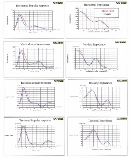
The above formulation has been applied to the determination of the impedances of an annular, rigid, massive foundation. The results for all six degrees of freedom, in frequency and time domains, are shown
in Figure 2. These results correspond to soil elastic constants: E=178000 kPa, ρ=1834.8 kg/m3, and
ν=1/3. The foundation has a outside radius of Ro=11.06m, thickness ∆R=2.5m, height h=2m, and mass
[image:10.612.84.528.140.680.2]density ρ=2550kg/m3.
Figure 2.
Impulse responses versus time and impedances versus frequency of a
DISCRETE MODEL FOR SOIL-FOUNDATION IMPEDANCES
[image:11.612.148.457.236.342.2]In order to minimize the computational effort, a set of discrete foundation springs and dashpots are introduced at the base of the foundation. They represent the discrete impedances of the soil-foundation system for all possible degrees of freedom of a rigid ring foundation of the type under consideration. However, the proposed procedure is general and can be applied for any type of foundation. According to this, the numerical results obtained in the previous section by the BEM-FEM methodology for the time and frequency domain responses of an ring foundation provide the basis for the determination of a 2-mass discrete model as the one shown in Figure 3. The computation of the proper combinations of mass, stiffness and damping constants is obtained via an automatic trial-and-error process programmed directly in the APDL programming language within ANSYS.
Figure 3. Discrete model for the computation of soil-foundation impedances.
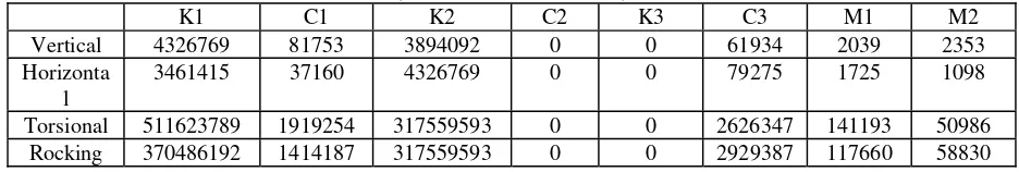
The results of this procedure are shown in Figure 2 for all possible modes of vibration of the rigid ring foundation under consideration. The corresponding discrete parameters (masses, springs and dampers) are listed in Table 1.
Table 1. Discrete parameters for approximate impedances in all six degrees of freedom (units in kN, m, and sec)
K1 C1 K2 C2 K3 C3 M1 M2
Vertical 4326769 81753 3894092 0 0 61934 2039 2353 Horizonta
l
3461415 37160 4326769 0 0 79275 1725 1098
Torsional 511623789 1919254 317559593 0 0 2626347 141193 50986 Rocking 370486192 1414187 317559593 0 0 2929387 117660 58830
ANALYSIS OF SPHERICAL TANK
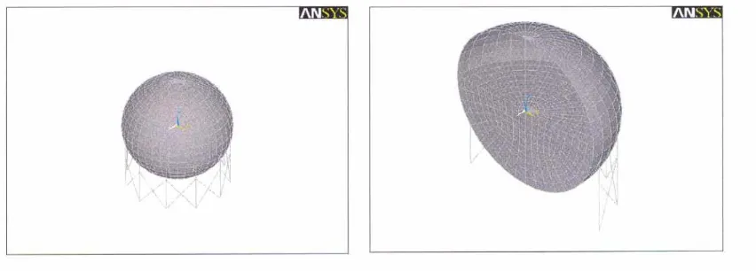
Some of the numerical results obtained from the analysis of a typical spherical tank using the proposed hybrid methodology are shown in this section. The outside radius of the tank is 20m, its average thickness is 4cm, and its equator stands at an elevation of 12.5m. It is supported by 11 columns of tube section with an outside diameter of 914.4mm and thickness 12.7mm. Lateral stiffness is provided by 11 pairs of bracings each one of which has a length of 8m and a cross section of 30x350mm. The tank is assumed to
contain propylene with bulk modulus 2GPa, and mass density 522kg/m3. The FE model for the structure,
[image:11.612.71.539.457.536.2]Figure 5. FEM model of spherical tank.
[image:12.612.69.546.329.439.2]The results from the modal analyses of the spherical tank assuming fixed base conditions or SSI are presented in Tables 1 and 2 for different levels of liquid fullness.
Table 2. Eigenvalues for fixed base conditions
Percentage of fluid fullness
Φ1 period, sec
(% modal mass participation)
Φ2 period, sec
(% modal mass participation)
Φ3 period, sec
(% modal mass participation)
50% 5
(41.7%)
0.25 (50%)
0.18 (8.3%)
75% 4.5
(26.6%)
0.32 (69%)
0.18 (4.4%)
98% 0.44
(98%)
0.18 (2%)
[image:12.612.67.547.489.600.2]0.11 (0.00%)
Table 3. Eigenvalues including SSI
Percentage of fluid fullness
Φ1 period, sec
(% modal mass participation)
Φ2 period, sec
(% modal mass participation)
Φ3 period, sec
(% modal mass participation)
50% 5
(14.7%)
0.3 (45%)
0.18 (39%)
75% 4.5
(11%)
0.32 (45%)
0.18 (42%)
98% 0.52
(59%)
0.18 (40%)
0.12 (0.00%)
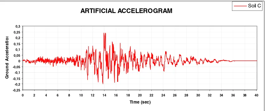
Subsequently, the transient response of the given structure to an artificial seismic excitation, shown in Figure 6, is computed. The seismic excitation is compliant to the spectral requirements of the Greek Seismic Code, for soil category C.
ARTIFICIAL ACCELEROGRAM
-0,25 -0,2 -0,15 -0,1 -0,05 0 0,05 0,1 0,15 0,2 0,25 0,3
0 2 4 6 8 10 12 14 16 18 20 22 24 26 28 30 32 34 36 38 40 Time (sec)
G
round
Ac
c
e
le
ra
ti
o
n
Soil C
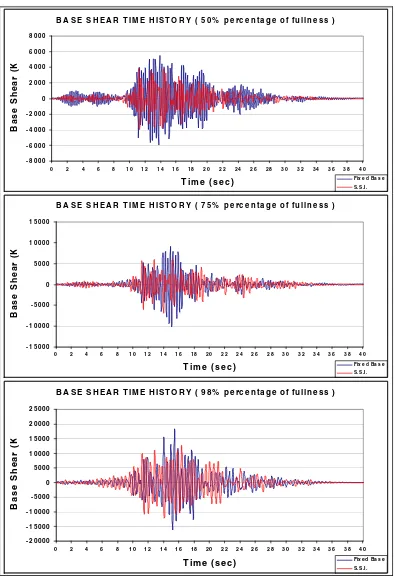
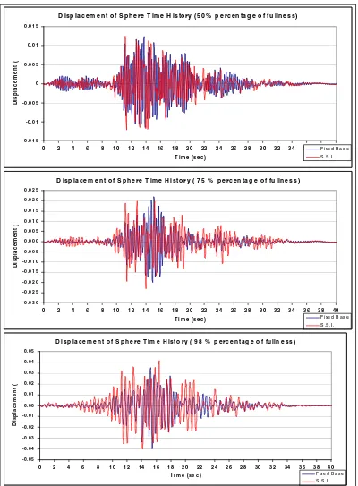
[image:13.612.89.519.131.310.2]values than those produced by fixed base boundary conditions. The opposite should be true for the displacement vs time plot. Figure 8 verifies this assumption, too.
Figure 6. Artificial accelerogram used for the analysis of spherical tank
CONCLUSIONS
An efficient hybrid BEM-FEM methodology in direct time domain is developed for the computation of the dynamic characteristics of massive foundations of arbitrary shape. The rigorous results obtained by the above methodology have been used for the determination of the discrete impedances of a rigid, ring foundation, on the basis of a 2 DOF model. Finally the complete seismic analysis of a typical spherical tank is attempted taking into consideration fluid-structure-soil interaction phenomena in direct time domain. For the structure–fluid portion of the entire model, standard FEM modeling is used coupled to the ANSYS pre- and post-processing modules. The proposed methodology can be easily extended to nonlinear dynamic analyses.
ACKOWLEDGEMENTS
Figure 7. Base shear (kN) versus time for various levels of fluid fullness.
B A S E S H E A R T IM E H I S T O R Y ( 5 0 % p e r c e n ta g e o f fu l ln e s s )
- 8 0 0 0 - 6 0 0 0 - 4 0 0 0 - 2 0 0 0 0 2 0 0 0 4 0 0 0 6 0 0 0 8 0 0 0
0 2 4 6 8 1 0 1 2 1 4 1 6 1 8 2 0 2 2 2 4 2 6 2 8 3 0 3 2 3 4 3 6 3 8 4 0 T im e ( s e c )
Ba
s
e
S
h
e
a
r
(
K
Fix e d Ba s e S .S . I.
B A S E S H E A R T IM E H I S T O R Y ( 7 5 % p e r c e n ta g e o f fu l ln e s s )
- 1 5 0 0 0 - 1 0 0 0 0 - 5 0 0 0 0 5 0 0 0 1 0 0 0 0 1 5 0 0 0
0 2 4 6 8 1 0 1 2 1 4 1 6 1 8 2 0 2 2 2 4 2 6 2 8 3 0 3 2 3 4 3 6 3 8 4 0 T im e ( s e c )
Ba
s
e
S
h
e
a
r
(
K
Fix e d Ba s e S .S . I.
B A S E SH E A R T IM E H IS T O R Y ( 9 8% p e rc e n ta g e o f fu lln e ss )
- 2 0 0 0 0 - 1 5 0 0 0 - 1 0 0 0 0 - 5 0 0 0 0 5 0 0 0 1 0 0 0 0 1 5 0 0 0 2 0 0 0 0 2 5 0 0 0
0 2 4 6 8 1 0 1 2 1 4 1 6 1 8 20 2 2 2 4 2 6 2 8 3 0 3 2 3 4 3 6 3 8 4 0 T im e (s e c )
B
a
s
e
S
h
ear
(
K
Figure 8. Displacement (m) at the top of the spherical tank versus time for various levels of fluid fullness
D is p la c e m e n t o f S p h e re T im e H is to ry (5 0 % p e rc e n ta g e o f fu lln es s )
-0 .0 1 5 -0 .0 1 -0 .0 0 5 0 0 .0 0 5 0 .0 1 0 .0 1 5
0 2 4 6 8 10 12 14 16 18 20 22 24 26 28 30 32 34 36 38 40
T im e (se c)
D
isp
lacem
e
n
t (
F i xe d B a s e S .S .I.
D is p la c e m e n t o f S p h e re T im e H is to ry ( 7 5 % p e rc e n ta g e o f fu lln e s s )
-0 .0 3 0 -0 .0 2 5 -0 .0 2 0 -0 .0 1 5 -0 .0 1 0 -0 .0 0 5 0 .0 0 0 0 .0 0 5 0 .0 1 0 0 .0 1 5 0 .0 2 0 0 .0 2 5
0 2 4 6 8 1 0 1 2 1 4 1 6 1 8 2 0 22 2 4 2 6 2 8 3 0 3 2 3 4 3 6 3 8 4 0 T i m e (se c )
D
is
p
lacem
en
t (
F i xe d B a s e S .S .I.
D is p la c e m e n t o f S p h e re T im e H is to ry ( 9 8 % p e rc e n ta g e o f fu lln e s s )
-0 .0 5 -0 .0 4 -0 .0 3 -0 .0 2 -0 .0 1 0 .0 0 0 .0 1 0 .0 2 0 .0 3 0 .0 4 0 .0 5
0 2 4 6 8 1 0 12 14 1 6 1 8 2 0 22 2 4 2 6 2 8 30 32 34 3 6 3 8 40 T i m e (se c )
D
isp
la
cem
e
n
t (
m
REFERENCES
1 Bathe K-J. “Finite element procedures in engineering analysis.” Englewood Cliffs, NJ:
Prentice-Hall, 1996.
2 Beskos DE. “Boundary element methods in dynamic analysis.” Applied Mechanics Review 1987;
40(1).
3 Beskos DE. “Boundary element methods in dynamic analysis: Part II 1986-1996.” ASME Applied
Mechanics Reviews 1997; 50(3): 149-197.
4 Karabalis DL, Beskos DE. “Dynamic response of 3-D rigid surface foundations by time domain
boundary element method.” Earthquake Engineering and Structural Dynamics 1984;12: 73-93.
5 Karabalis DL, Beskos DE. “Dynamic response of 3-D flexible foundations by time domain BEM
and FEM.” Soil Dynamics and Earthquake Engineering 1985; 4: 91-101.
6 Karabalis DL, Beskos DE. “Dynamic response of 3-D embedded foundations by the boundary
element method.” Computer Methods in Applied Mechanics and Engineering 1986; 56: 91-119.
7 Karabalis DL, Beskos DE. “Dynamic soil–structure interaction.” Beskos DE. Editor. Boundary
Element Methods in Mechanics. Amsterdam: North Holland, 1987.
8 Markerle J. “FEM and BEM in geomechanics: foundations and soil-structure interaction – a
bibliography (1992 –1994).” Finite Elements In Analysis and Design 1996; 22(3): 249 – 263.
9 Rizos DC. “3-D direct time domain BEM in elastodynamic.” Ph.D Thesis, Columbia: Univ. of
South Carolina 1993.
10 Rizos DC. “A rigid surface boundary element for 3D soil-structure interaction analysis in the direct
time domain.” Computational Mechanics2000.
11 Rizos DC, Karabalis DL. “An advanced direct time domain BEM formulation for general 3-D elastodynamic problems.” Computational Mechanics 1994; 15: 249-269.
12 Rizos DC, Karabalis DL. “A time domain BEM for 3-D elastodynamic analysis using the B-Spline fundamental solutions.” Computational mechanics 1998; 15: 249-269.
13 Rizos DC, Karabalis DL. “Soil-fluid-structure interaction.” Kausel E, Manolis GD. Editors. Wave Motion Problems in Earthquake Engineering. Southampton: WIT Press, 1999.
14 Rizos DC, Loya KG. “Dynamic and seismic analysis of foundations based on free field B-Spline
characteristic response histories.”Journal of Engineering Mechanics ASCE2001.