A Direct Approach for Determining the Switch
Points in the Karnik-Mendel Algorithm
Chao Chen,
Student Member, IEEE,
Robert John,
Senior Member, IEEE,
Jamie Twycross
and Jonathan M. Garibaldi,
Member, IEEE
Abstract—The Karnik-Mendel algorithm is used to compute the centroid of interval type-2 fuzzy sets, determining the switch points needed for the lower and upper bounds of the centroid, through an iterative process. It is commonly acknowledged that there is no closed-form solution for determining such switch points. Many enhanced algorithms have been proposed to improve the computational efficiency of the Karnik-Mendel algorithm. However, all of these algorithms are still based on iterative procedures. In this paper, a direct approach based on derivatives for determining the switch points without multiple iterations has been proposed, together with mathematical proof that these switch points are correctly determining the lower and upper bounds of the centroid. Experimental simulations show that the direct approach obtains the same switch points, but is more computationally efficient than any of the existing (iterative) algorithms. Thus, we propose that this algorithm should be used in any application of interval type-2 fuzzy sets in which the centroid is required.
Index Terms—Karnik-Mendel algorithm, centroid, interval type-2, fuzzy sets, iterative, closed-form, direct approach.
I. INTRODUCTION
T
HE Karnik-Mendel (KM) algorithm was the first algo-rithm proposed to determine the switch points when computing the centroids of interval type-2 (IT2) fuzzy sets [1]. With its fast convergence, it is still the most widely used algorithm for computing the switch points [2, 3, 4, 5, 6]. It was originally shown that the maximum number of iterations of the KM algorithm is N, which is the number of discrete points in the universe of discourse for an IT2 fuzzy set. This was believed to be extremely conservative and it was subsequently proved by Liu [7] that the maximum number of iterations of the KM algorithm is(N+ 1)/2. A much smaller number(N+ 2)/4 was given in [8] as the maximum number of iterations, without proof. Though these numbers are much smaller than N, they are still believed to be conservative [3]. Many studies by simulations show that the KM algorithm converges in from two to six iterations, regardless of N [9].Many attempts have been made to improve the efficiency of the KM algorithm. The enhanced KM (EKM) algorithm introduces a better initialisation, which “on average ... can save
The authors are with the Laboratory for Uncertainty in Data and Decision Making (LUCID), the Intelligent Modelling and Analysis (IMA) and the Automated Scheduling Optimisation and Planning (ASAP) Research Groups, School of Computer Science, University of Nottingham, Nottingham, Jubilee Campus, NG8 1BB UK e-mail: {chao.chen, robert.john, jamie.twycross, jon.garibaldi}@nottingham.ac.uk.
Manuscript received *** **, 2016; revised *** **, 2017; accepted *** **, 2017. Date of publication *** **, 2017; date of current version *** **, 2017.
Digital Object Identifier ***
about two iterations” [9]. Also, some algorithmic improve-ments to simplify computations were introduced to reduce the computational cost for each iteration. An improved iterative algorithm with stopping condition (IASC) was first proposed in [10] and further refined in [11]. Further improvements to the IASC have been made in the enhanced IASC (EIASC) in [12]. Both the IASC and EIASC algorithms have been reported to be superior to the KM and EKM algorithms whenN is small (e.g.N 6100). However, their computational costs increase rapidly asN increases since many possible switch points have to be evaluated before finding the correct ones [3].
Rather than calculating the exact centroids, closed-form solutions, which are much more efficient than iterative algo-rithms, have been provided for approximations. For example, the Nie-Tan (NT) method as given in [13]. It has been demonstrated that the NT method can give a very good approximation to the KM algorithm. As an extension of the NT method, a better approximation with Taylor-series is provided in [14]. Closed-form formulae for calculating the centroids of a general type-2 fuzzy set are proposed in [15], where linear connections between the centroid endpoints of any α plane and that of α = 0 andα = 1 planes have been introduced. However, the calculations of the centroid end points of the
α= 0 andα= 1 planes are still based on the iterative KM algorithm. Other algorithms to improve efficiency have also been proposed recently, such as [16] and [17], although these too are iterative.
To the best of our knowledge, all existing algorithms, such as the EKM and the EIASC, for determining the switch points are iterative-based methods. In this paper, a direct approach which can compute the switch points based on derivatives, without multiple iterations, is proposed. We use the term ‘iteration’ here to mean the repeated calculation of the position of the switch points. Within all approaches there are common calculations that require looping (e.g. cumulative sum), which we do not consider as iterations of the main algorithm.
II. THEKMALGORITHM
Let an IT2 fuzzy set A˜be based on
xi ∈X, i= 1,2, ..., N Ji≡[
¯ui,ui¯], 06¯ui 6ui¯ 61
where xi is the primary variable in the discrete universe of
discourse X (note that xi is in ascending order for i from
1 to N),Ji represents the membership grade interval for the
primary variable xi, and N is the number of discrete points
in the universe of discourse.
For any given embedded type-1 fuzzy set, with membership grades ui ∈ Ji for all i, of such an IT2 fuzzy set A˜, the centroid is defined as:
c =
PN
i=1xiui PN
i=1ui .
If the above centroid cis computed for all embedded type-1 fuzzy sets, a centroid interval C= [cl, cr] can be obtained where
cl = inf
∀ui∈Ji PN
i=1xiui PN
i=1ui
cr = sup
∀ui∈Ji PN
i=1xiui
PN
i=1ui
In fact, there is no need to compute the centroids for all embedded type-1 fuzzy sets to get the centroid interval. It is well known that the endpointsclandcrof the centroid interval can also be expressed as (the derivation can be found in [9]):
cl =
PL
i=1xiui¯ + PN
i=L+1xi¯ui PL
i=1ui¯ + PN
i=L+1¯ui
(1)
cr =
PR
i=1xi
¯
ui+P N
i=R+1xiu¯i
PR
i=1¯ui+ PN
i=R+1ui¯
(2)
where L and R, which are integer indices in the range of
[1, N−1], are the switch points for selecting
¯
ui or ui¯. As stated by Mendel [3], there is no closed-form solution for such switch points LandR, and hence, forclandcr. By utilising the properties of the switch points such that
xL6cl6xL+1
xR6cr6xR+1
the KM algorithm can be used to find them iteratively [1].
III. THE ITERATIVE ALGORITHMS
In this section, two commonly used iterative algorithms are briefly introduced, to establish terminology and notation. Rather than introduce the original KM and IASC algorithms, their enhancements (the EKM and EIASC algorithms) are re-viewed as they are more efficient than the original algorithms.
A. The EKM algorithm
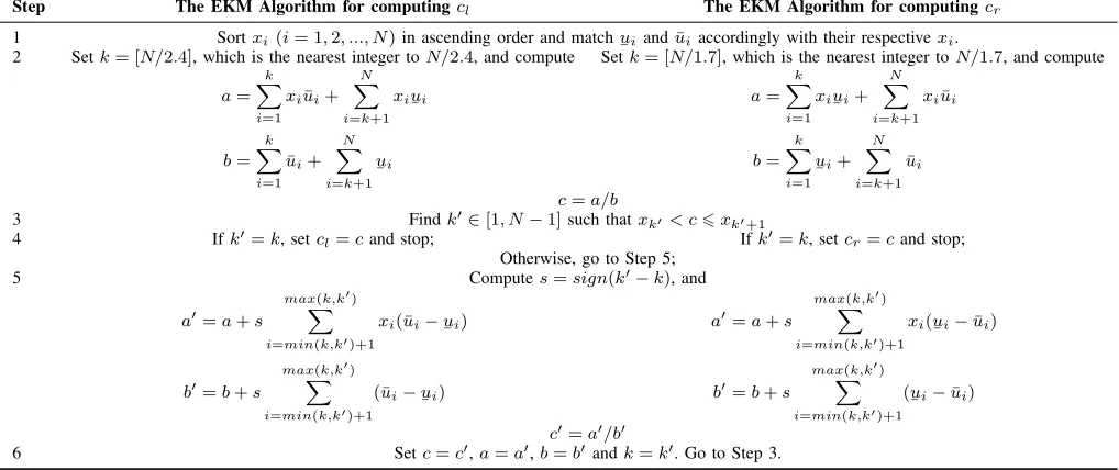
The EKM algorithm is summarised in Table I. Compared to the original KM algorithm, the EKM algorithm introduces a better initialisation (Step 2) for the starting position and a change of the termination condition (Step 4) to remove an unnecessary iteration [9]. The EKM algorithm can save, on average, about two iterations. Simplified calculations (Step 5) are also introduced to save computational costs for each iteration.
B. The EIASC algorithm
The EIASC algorithm is summarised in Table II. Compared to the original IASC algorithm, the EIASC algorithm intro-duced a new stopping criterion (Step 4) [12]. Also, the starting point for computingcr has been changed toN (Step 2) since the switch point R for cr has been shown to be generally greater than N/2[9].
IV. THEDIRECTAPPROACH(DA)ALGORITHM
An arbitrary c in the centroid interval C, represented as Equation 3, can be expanded to Equation 4. Equation 4 can then be transformed to Equation 5 by substituting x1+ Pi
j=2δxj for all correspondingxi(i >1), where δxj =xj−xj−1.
For example,x3 in Equation 4 is represented as(x1+δx2+
δx3) in Equation 5. Note that δxj is always positive since
xi (defined in Section II), and hence xj, is in ascending order. This transformation is made to allow the sign of the partial derivatives to be easily identified, as shown in Equations 7 to 11. After the transformation, by rearranging and aggregating all the items with x1 andδxj for j= 2,3, ..., N
in Equation 5,ccan finally be represented as Equation 6. We can then compute the partial derivative ofcwith respect touj
in the pattern of Equations 7 to 8. Then, this partial derivative
∂c
∂uj can be represented as Equation 9 for specific j∈[1, N].
It is noted by Karnik and Mendel [1] and Wu and Mendel [9] that equating the partial derivative ofc with respect touj
to zero does not give us any information about the value ofuj
that maximises or minimisesc. However, it can be observed that the sign of the partial derivative of c with respect to uj
does not depend on the value of uj. Hence, it is clear that,
when the partial derivative is negative, it is necessary to take the largest possible value ofuj in order to minimisec. When the partial derivative is positive, it is necessary to take the smallest possible value ofujin order to minimisec. That is, to obtaincl(the minimum centroid), one must setuj touj¯ when the partial derivative is negative, and to
¯
uj when the partial derivative is positive. We observe that for any given value of
uj, this partial derivative is monotonically increasing with j
(from 1 to N). Hence, for cl, there must be a switch point
k∈[1, N] for which ∂u∂c
k ≤0 and
∂c
∂uk+1 ≥0. Based on the above, it is possible to find the switch point directly by locating the value ofkwhere the sign of the partial derivative changes. The same principles can be used to find the switch pointkfor the maximum centroidcr, swappinguj¯ and
¯
Step The EKM Algorithm for computingcl The EKM Algorithm for computingcr
1 Sortxi(i= 1,2, ..., N)in ascending order and match
¯
uiandu¯iaccordingly with their respectivexi.
2 Setk= [N/2.4], which is the nearest integer toN/2.4, and compute Setk= [N/1.7], which is the nearest integer toN/1.7, and compute
a=
k
X
i=1 xi¯ui+
N
X
i=k+1 xi
¯
ui
b=
k
X
i=1
¯
ui+ N
X
i=k+1¯ ui
a=
k
X
i=1 xi
¯
ui+ N
X
i=k+1 xiu¯i
b=
k
X
i=1¯ ui+
N
X
i=k+1
¯
ui
c=a/b
3 Findk0∈[1, N−1]such thatxk0 < c6xk0+1
4 Ifk0=k, setcl=cand stop; Ifk0=k, setcr=cand stop;
Otherwise, go to Step 5;
5 Computes=sign(k0−k), and
a0=a+s
max(k,k0) X
i=min(k,k0)+1 xi(¯ui−
¯
ui)
b0=b+s
max(k,k0) X
i=min(k,k0)+1
(¯ui−
¯
ui)
a0=a+s
max(k,k0) X
i=min(k,k0)+1 xi(
¯
ui−¯ui)
b0=b+s
max(k,k0) X
i=min(k,k0)+1
( ¯
ui−u¯i)
c0=a0/b0
[image:3.612.52.561.57.271.2]6 Setc=c0,a=a0,b=b0andk=k0. Go to Step 3.
TABLE I: The EKM algorithm for computing the centroid end points (cl and cr) of an IT2 Fuzzy Set. Note that for the case described in Section II, Step 1 is not necessary sincexi has already been defined in ascending
order. Table I is adapted from [3, 9].
Step The EIASC Algorithm for computing cl The EIASC Algorithm for computing cr
1 Sortxi (i= 1,2, ..., N)in ascending order and match
¯
ui and u¯i accordingly with their respective xi.
2 Initialise k= 0 and Initialisek=N and
a=
N X
i=1
xi
¯ui
b=
N X
i=1¯
ui
3 Computek=k+ 1 Compute
a=a+xk(¯uk−
¯ uk)
b=b+ ¯uk−
¯ uk
c=a/b
k=k−1
4 If c6xk+1, set cl =c and stop; Ifc >xk, set cr =c and stop; Otherwise, go to Step 3;
TABLE II: The EIASC algorithm for computing the centroid end points (cl andcr) of an IT2 Fuzzy Set. Note
that for the case described in Section II, Step 1 is not necessary sincexi has already been defined in ascending
order. Table II is adapted from [3, 12].
c with respect to each uj, and hence providing a method for
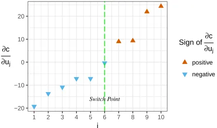
directly obtaining the switch points. Figure 1 illustrates the monotonically increasing trend of the partial derivative ∂u∂c
j
and the location of the switch point.
Since δxj is always positive, it can be observed in Equa-tion 9 that the partial derivative consists of two parts, which are the positive part posj and the negative partnegj:
∂c
∂uj =posj+negj
where posj andnegj are presented in Equations 10 and 11,
which can be summarised as Equations 12 and 13. Having all the partial derivatives, the switch points L for cl and R
for cr can be obtained as follows.
ForL and hence cl:
1) Calculateposjby setting all theuito beui¯ and calculate
negj by setting all theui to be
¯
ui, for allj∈[1, N]. 2) Calculate all the partial derivatives ∂u∂c
j asposj +negj.
3) Find the smallestk∈[1, N−1]such that ∂u∂c
[image:3.612.54.556.331.549.2]Switch Point
−20 −10 0 10 20
1 2 3 4 5 6 7 8 9 10
j ∂c
∂uj
Sign of ∂c ∂uj
positive
[image:4.612.63.287.55.187.2]negative
Fig. 1: An illustration of the DA algorithm showing the position of the switch point for an arbitrary example where
N is 10.
For R and hence cr:
1) Calculateposjby setting all theuito be
¯
uiand calculate
negj by setting all theui to beui¯ , for allj∈[1, N]. 2) Calculate all the partial derivatives ∂u∂c
j asposj +negj.
3) Find the largest k∈[1, N−1]such that ∂u∂c
k 60.
4) If kexists, set R=k; otherwise, setR= 1. 5) Compute cr by Equation 2.
It should be noted that the denominator (PN
i=1ui)2 in
Equations 12 and 13, which must be positive, can be neglected in calculations to save computational costs. In other words, without the risk of changing the sign of ∂u∂c
j,posj andnegj
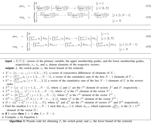
can be simplified as presented in Equations 14 and 15. Also, in practice, there is no need to calculate the partial derivatives one by one, as cumulative sums and vectorised operations can be used. The pseudo-code for obtaining L and cl is shown
in Algorithm 1. Randcr are calculated in a similar manner, making the substitutions as described above (pseudo-code is omitted due to space constraints).
V. PROOF OF THEDAALGORITHM
Proposition 1. It is clear that when ∂u∂c
j <0,uj should be
its maximum value, uj¯ , to minimise c and it should be its minimum value,
¯
uj, to maximisec. Conversely, when∂u∂c
j >0,
ujshould be
¯ujto minimisecand it should beu¯j to maximise
c. When ∂u∂c
j = 0,cis not dependent on the value of uj.
Theorem 1. The index L obtained by the DA algorithm,
as described in Section IV, is the correct switch point for calculating the minimum centroid cl.
Proof. Given that δxi is always positive, it is clear (from
Equations 14 and 15) that for any j∈[1, N],posj attains its
maximum value whenui isui¯ andnegj attains its maximum value when ui is
¯ui; hence
∂c
∂uj is also maximal. It can be
observed from Equation 8 that ∂u∂c
j is monotonically increasing
inj. This is because the only difference of ∂u∂c
j forj=n−1
andj=nis the nthterm (n∈[2, N]), which is negative for j =n−1and positive for j=n.
If there exists a smallestk∈[1, N−1]such that ∂u∂c
k+1 >0, thenkis the correct switch pointL(for calculatingcl) on the basis that:
1) L cannot be less than k, for the following reason. For every j ∈ [1, k], it must be the case that ∂u∂c
j < 0.
Therefore, by proposition 1,uj should be its maximum value u¯j to minimisec. Now suppose Lis less than k.
Then, asL is the switch point, everyuj∈[L+1,k] should
be its minimum value
¯
uj, which by contradiction is not
possible.
2) L cannot be greater than k, for the following reason. Assume L is greater than k. Then, as L is the switch point everyuj∈[k+1,L] should be its maximum valueuj¯ .
By proposition 1, it must be the case that ∂u∂c
k+1 <0, in which caseuk+2 must be changed from
¯uk+2 touk¯ +2.
This means ∂u∂c
k+2, if it exists, must also be negative. By induction, it can be deduced that ∂u∂c
N must be negative.
This is in contradiction to the fact that ∂u∂c
N > 0. Thus,
the assumption is incorrect. Hence,Lcannot be greater thank.
If there does not exist ak∈[1, N−1]such that ∂u∂c
k+1 >0, then for every j ∈[1, N−1], again it must be the case that
∂c
∂uj <0. Also,
∂c
∂uN must be 0. Thus, there is no contradiction
for the switch pointL to beN−1.
Theorem 2. The index R obtained by the DA algorithm,
as described in Section IV, is the correct switch point for calculating the maximum centroid cr.
Proof. The proof is similar to above.
VI. EXPERIMENTAL COMPARISON
To further investigate the performance of the new DA, com-parisons in terms of time efficiency between the new approach and two of the most widely used algorithms (the EKM and the EIASC algorithms) were conducted. The platform was a laptop with Intel Core i7-3720QM CPU @ 2.60GHz and 8GB memory, running Windows 7 Professional 64bit Service Pack 1. The programming language and software environment is R x64 version 3.2.3. Computational costs were measured by the user time returned by the built-in function proc.time() in the R environment.
A. Examples of IT2 fuzzy sets
In this section, three example IT2 fuzzy sets are used to verify the correctness of the DA algorithm by comparing the switch points with the EKM algorithm and the EIASC algorithm. Specifically, the vector X, containingxi, has 101 discrete values from 0 to 10 by a step size of 0.1. ui¯ and
¯
ui
are obtained by the following membership functions for each type of example IT2 fuzzy sets.
1) Symmetric Gaussian membership functions with uncer-tain deviation:
¯
ui = exp −0.5
x
i−5
1.75
2!
¯ui = exp −0.5
xi−5
0.25
c =
PN
i=1xiui PN
i=1ui
(3)
= x1u1+x2u2+x3u3· · ·+xNuN
PN
i=1ui
(4)
= x1u1+ (x1+δx2)u2+ (x1+δx2+δx3)u3· · ·+ (x1+δx2· · ·+δxN)uN
PN
i=1ui
(5)
= x1+
(PN
i=2ui)δx2 PN
i=1ui
+(
PN
i=3ui)δx3 PN
i=1ui
· · ·+(
PN
i=Nui)δxN
PN
i=1ui
(6)
∂c ∂uj
= ∂
∂uj
x1+
(PN i=2ui)δx2
PN i=1ui
+( PN
i=3ui)δx3
PN i=1ui
· · ·+( PN
i=Nui)δxN PN
i=1ui !
(7)
= ∂
∂uj (x1) +
∂ ∂uj
(PNi=2ui)δx2
PN i=1ui
! + ∂
∂uj
(PNi=3ui)δx3
PN i=1ui
!
· · ·+ ∂
∂uj
(PNi=Nui)δxN PN
i=1ui ! (8) = 0−
(PN i=2ui)δx2 (PN
i=1ui)2
−( PN
i=3ui)δx3 (PN
i=1ui)2
−( PN
i=4ui)δx4 (PN
i=1ui)2
· · · −( PN
i=N−2ui)δxN−2 (PN
i=1ui)2
−( PN
i=N−1ui)δxN−1 (PN
i=1ui)2
−( PN
i=Nui)δxN
(PN i=1ui)2
j= 1
0 +
(P1
i=1ui)δx2 (PN
i=1ui)2
−( PN
i=3ui)δx3 (PN
i=1ui)2
−( PN
i=4ui)δx4 (PN
i=1ui)2
· · · −( PN
i=N−2ui)δxN−2 (PN
i=1ui)2
−( PN
i=N−1ui)δxN−1 (PN
i=1ui)2
−( PN
i=Nui)δxN
(PN i=1ui)2
j= 2
0 +
(P1
i=1ui)δx2 (PN
i=1ui)2 +(
P2
i=1ui)δx3 (PN
i=1ui)2
−( PN
i=4ui)δx4 (PN
i=1ui)2
· · · −( PN
i=N−2ui)δxN−2 (PN
i=1ui)2
−( PN
i=N−1ui)δxN−1 (PN
i=1ui)2
−( PN
i=Nui)δxN
(PN i=1ui)2
j= 3
. . .
0 +
(P1
i=1ui)δx2 (PN
i=1ui)2 +(
P2
i=1ui)δx3 (PN
i=1ui)2 +(
P3
i=1ui)δx4 (PN
i=1ui)2
· · ·+(
PN−3
i=1 ui)δxN−2 (PN
i=1ui)2
−( PN
i=N−1ui)δxN−1 (PN
i=1ui)2
−( PN
i=Nui)δxN
(PN i=1ui)2
j=N−2
0 +
(P1
i=1ui)δx2 (PN
i=1ui)2 +(
P2
i=1ui)δx3 (PN
i=1ui)2 +(
P3
i=1ui)δx4 (PN
i=1ui)2
· · ·+(
PN−3
i=1 ui)δxN−2 (PN
i=1ui)2 +(
PN−2
i=1 ui)δxN−1 (PN
i=1ui)2
−( PN
i=Nui)δxN
(PN i=1ui)2
j=N−1
0 +
(P1
i=1ui)δx2 (PN
i=1ui)2 +(
P2
i=1ui)δx3 (PN
i=1ui)2 +(
P3
i=1ui)δx4 (PN
i=1ui)2
· · ·+(
PN−3
i=1 ui)δxN−2 (PN
i=1ui)2 +(
PN−2
i=1 ui)δxN−1 (PN
i=1ui)2 +(
PN−1
i=1 ui)δxN (PN
i=1ui)2
j=N
(9) posj =
0 j= 1
0 + (
P1
i=1ui)δx2
(PN i=1ui)2
j= 2
0 + (
P1
i=1ui)δx2
(PN i=1ui)2
+(
P2
i=1ui)δx3
(PN i=1ui)2
j= 3
.. .
0 + (
P1
i=1ui)δx2
(PN
i=1ui)2 + (P2
i=1ui)δx3
(PN
i=1ui)2 · · ·+
(PNi=1−3ui)δxN−2
(PN i=1ui)2
j=N−2
0 + (
P1
i=1ui)δx2
(PN
i=1ui)2 + (P2
i=1ui)δx3
(PN
i=1ui)2 · · ·+
(PNi=1−2ui)δxN−1
(PN i=1ui)2
j=N−1
0 + (
P1
i=1ui)δx2
(PN i=1ui)2
+(
P2
i=1ui)δx3
(PN i=1ui)2
· · ·+(PN
−1
i=1 ui)δxN (PN
i=1ui)2
j=N
(10) negj =
−(PNi=2ui)δx2
(PN
i=1ui)2 · · · −
(PNi=N−1ui)δxN−1
(PN
i=1ui)2 −
(PNi=Nui)δxN (PN
i=1ui)2 j= 1
−(PNi=3ui)δx3
(PN i=1ui)2
· · · −(PNi=N−1ui)δxN−1
(PN i=1ui)2
−(PNi=Nui)δxN (PN
i=1ui)2
j= 2
−(PNi=4ui)δx4
(PN
i=1ui)2 · · · −
(PNi=N−1ui)δxN−1
(PN
i=1ui)2 − (PN
i=Nui)δxN (PN
i=1ui)2 j= 3
.. .
−(
PN
i=N−1ui)δxN−1
(PN
i=1ui)2 −
(PNi=Nui)δxN (PN
i=1ui)2
j=N−2
−(PNi=Nui)δxN (PN
i=1ui)2
j=N−1
0 j=N
posj =
(
0
j= 1 (P1
i=1ui)δx2
(PNi=1ui)2
h
+(
P2
i=1ui)δx3
(PNi=1ui)2 · · ·+
(Pji=1−1ui)δxj (PNi=1ui)2
i
j∈[2, N]
(12)
negj =
−(
PN
i=j+1ui)δxj+1
(PN
i=1ui)2 · · · −
(PNi=N−1ui)δxN−1
(PN i=1ui)2
−(PNi=Nui)δxN (PN
i=1ui)2
j ∈[1, N−1]
0 j =N
(13)
posj =
(
0 j= 1
P1
i=1ui
δx2 h
+P2
i=1ui
δx3· · ·+
Pj−1
i=1ui
δxji j∈[2, N]
(14)
negj =
(h
−PN
i=j+1ui
δxj+1· · · −
PN
i=N−1ui
δxN−1 i
−PN
i=Nui
δxN
j ∈[1, N−1]
0 j =N
(15)
input : X,U,¯
¯
U, vectors of the primary variable, the upper membership grades, and the lower membership grades, respectively;xi,u¯i, and
¯ui denote elements of the respective vectors;
output: L, the switch point;cl, the lower bound of the centroid;
1 X0← {xi−xi−1|i= 2,3, ..., N}, a vector of consecutive differences of elements ofX ;
2 S1 ← {Pji=1ui¯ |j= 1,2, ..., N−1}, a vector of the cumulative sum of the firstN−1 elements ofU¯ ; 3 S2 ← {Pji=N
¯ui|j=N, ...,3,2}a vector of the cumulative sum of the last N−1 elements of¯U in the reverse
order ;
4 TP ← {xi0·si1 |i= 1,2, ..., N−1}, where xi0 andsi1 are theithelement of vectors X0 andS1 respectively ; 5 TN ← {xN0 −i·si2 |i= 1,2, ..., N−1}, wheresi2 is the ith element of the vectorS2 ;
6 DP ← {0,Pji=1tiP |j= 1,2, ..., N−1}, where tiP is theithelement of the vectorTP ; 7 DN ← {Pji=1−tiN,0|j =N−1, ...,2,1}, where tiN is the ithelement of the vector TN ; 8 D← {diP+diN |i= 1,2, ..., N}, where dP
i anddiN are theithelement of vectors DP andDN respectively ;
9 Find the smallest k∈1,2, ..., N−1 such thatdk+1>0, where dk+1, which represents ∂cl
∂uk+1, is the(k+ 1)
th
element of the vectorD ;
10 if kexiststhen L←k elseL←N−1; 11 Computecl by Equation 1;
Algorithm 1: Pseudo code for obtainingL, the switch point; and cl, the lower bound of the centroid.
2) Gaussian upper membership function and triangular lower membership function:
¯
ui =
exp−0.5 xi−2
5
2
06xi67.185
exp−0.5 xi−9
1.75 2
7.185< xi610
¯
ui =
(0.6(xi+5) 19
06xi62.6 0.4(14−xi)
19
2.6< xi 610
3) Piecewise Gaussian membership functions:
¯
ui = max
exp
−x√i−3 8
2
0.8 exp
−x√i−6 8
2
¯
ui = max
0.5 exp
−x√i−3 2
2
0.4 exp
−x√i−6 2
2
As shown in Table III, the switch pointsL andR obtained with the examples by three algorithms are all the same.
Example 1 Example 2 Example 3
L R L R L R
DA 36 65 27 69 32 57
EKM 36 65 27 69 32 57
[image:6.612.51.564.59.479.2]EIASC 36 65 27 69 32 57
TABLE III: The switch points L andR obtained by three algorithms based on the example fuzzy sets.
B. Generalised IT2 fuzzy sets
1) Generalised bell-shaped IT2 fuzzy sets: It was assumed that the vectorX, containingxi, is uniformly distributed from
0 to 10. u¯i and
¯
ui are defined by generalised bell-shaped
function:
¯
ui = 1
1 + xi−c
¯
a
2b
¯
ui = 1
1 +xi−c
¯
a
where
¯a andb are randomly selected between 1 and 2; ¯a is
the multiplication of
¯
awith a random number between 1 and 2;c is a random number between 0 and 10.
2) Generalised randomly-shaped IT2 fuzzy sets: This ex-perimental comparison was designed to be similar to the first comparison in [12]. It was assumed that vectors X and U¯, containing xi and ui¯ respectively, are uniformly distributed from 0 to 1.
¯
ui is the multiplication of ui¯ with a random number between 0 and 1.
Comparisons are made for these two types of IT2 fuzzy sets separately. In each comparison,N, which is the length ofX, is set to be between 10 and 2000 with a step size of 10 (giving 200 different values ofN). For each value ofN, 5000 Monte Carlo simulations were made and the computational time costs were aggregated to be compared for each algorithm.
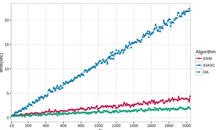
In all the 2×10⁶ simulations, the DA algorithm gave the same switch points as those given by the KM and the EIASC algorithms. Computational time comparisons are shown in Figures 2 and 3. It can be observed that the three algorithms compared are similar whenN is very small. It should be noted that the EIASC algorithm is shown to be better than the EKM algorithm when N is smaller than 1000 [12]. However, in our experiments, the EIASC algorithm is only more efficient than other algorithms when N is around 10. In contrast, DA clearly outperforms other algorithms when N is larger than 100 regardless of the shape of fuzzy sets.
VII. DISCUSSION
As can be observed in Figures 2 and 3, the computational time of the EIASC algorithm increases most rapidly among the three algorithms. As has already been discussed, this is because the number of switch points to be evaluated for the EIASC algorithm increases along with the increase of N. In other words, the number of iterations for the EIASC algorithm increases rapidly. In contrast, the EKM algorithm can achieve its final result in from two to six iterations, regardless of N. Thus, the computational time for the EKM algorithm increases less significantly than the EIASC algorithm. However, the computational time does increase linearly because the size of the vectors involved in the computing process increases along with the increase of N.
Regardless of the shape of fuzzy sets, our newly proposed DA algorithm performs the best among the three algorithms, although it can be considered as a brute-force approach since all the partial derivatives have to be computed before locating the switch points. However, vectorised operations and the use of cumulative sum make the computing of partial derivatives quite simple. Thus, the DA algorithm is still competitive for very small values ofN and clearly outperforms the EKM, the EIASC for N & 100.
VIII. CONCLUSION
In this paper, a direct approach based on derivatives for determining the switch points for calculating the centroid of an interval type-2 fuzzy set has been introduced. A derivation of the algorithm, psuedo-code for calculating the switch points, and a mathematical proof of correctness of the switch points
●●●●●●●●●●●●●●●● ●●●●●●●●●●●●●●●●●●●●●●●●●●●
● ●●●●●●●
●●●●●●●●●●●●●●●●●●●●● ●
●●●●●●●●●●● ●●●
●● ●● ●●●●●●●
●●●●● ● ●●●●
● ●●●●●●●●●●
●●● ● ●●●●●
● ● ● ● ●●●
●●● ● ●●●●
●● ●●●
●● ●● ●●●
● ●●●●●
● ● ● ●●
●●●●●●●●●●●● ● ● ● ●●
● ●●●●●●
● ●●●●●●●●●●●
● ●
0 5 10 15 20
10 200 400 600 800 1000 1200 1400 1600 1800 2000
N
time(sec)
Algorithm
● EKM
[image:7.612.326.548.62.195.2]EIASC DA
Fig. 2: A comparison of computational time costs for different algorithms based on generalised bell-shaped IT2 fuzzy sets described in Section VI.
●●●●●●●●●●●●●●●●●●●●●●●●● ●●●
●●●● ●●●●
●●●●●● ●●●●●
●●●●●●●●●●●●●● ● ●● ●●
● ●●
●●●●●●● ●●●●●●●
● ● ●●●
●●● ●● ●●●●●
●●●●●●● ●●●●●●
● ● ●● ● ●●
● ●●
● ●●●●●
● ●●●●●●●●
●● ● ● ● ● ● ● ●●●
●●● ●●
● ● ●●
● ●●●●●●●●
● ● ●●●●●
●●● ●●●●●●
●● ● ●●●●
● ●●
●●●● ●●●●
●●● ● ●
0 5 10 15 20
10 200 400 600 800 1000 1200 1400 1600 1800 2000
N
time(sec)
Algorithm
● EKM
EIASC DA
Fig. 3: A comparison of computational time costs for different algorithms based on generalised randomly-shaped IT2 fuzzy sets described in Section VI.
have been given for the proposed approach. By empirical simulations, it has been shown that DA is superior to all other iterative algorithms (including the EKM and the EIASC) in time efficiency. It should be noted that the DA algorithm is in fact a brute force method which requires the calculations of all partial derivatives. While it can be noted that the partial derivatives are in ascending order and the switch points are located where the sign of partial derivatives changes, it would be interesting for an approach to find the switch points without calculating all the partial derivatives.
In conclusion, we have contributed a new algorithm for determining the switch points for calculating the lower and upper bounds of the centroids of an interval type-2 fuzzy set. Given that our algorithm clearly outperform the EKM and the EIASC algorithms, we suggest that this new DA algorithm should always be used whenN, the number of discretizations of the universe of discourse,&100.
REFERENCES
[1] N. Karnik and J. Mendel, “Centroid of a type-2 fuzzy set,” Information Sciences, vol. 132, no. 14, pp. 195– 220, 2001.
[3] J. Mendel, H. Hagras, W.-W. Tan, W. W. Melek, and H. Ying, Introduction To Type-2 Fuzzy Logic Control: Theory and Applications, 1st ed. Wiley-IEEE Press, 2014.
[4] J. M. Mendel and M. R. Rajati, “On Computing Normal-ized Interval Type-2 Fuzzy Sets,”IEEE Transactions on Fuzzy Systems, vol. 22, no. 5, pp. 1335–1340, 2014. [5] M. Nie and W. W. Tan, “Ensuring the Centroid of an
Interval Type-2 Fuzzy Set,”IEEE Transactions on Fuzzy Systems, vol. 23, no. 4, pp. 950–963, 2015.
[6] T. Kumbasar, “Revisiting KM algorithms: A Linear Pro-gramming approach,” inProceedings IEEE International Conference on Fuzzy Systems, 2015, pp. 1–6.
[7] F. Liu and J. M. Mendel, “Aggregation using the fuzzy weighted average as computed by the Karnik-Mendel al-gorithms,”IEEE Transactions on Fuzzy Systems, vol. 16, no. 1, pp. 1–12, 2008.
[8] H. Wu and J. M. Mendel, “Uncertainty bounds and their use in the design of interval type-2 fuzzy logic systems,” IEEE Transactions on Fuzzy Systems, vol. 10, no. 5, pp. 622–639, 2002.
[9] D. Wu and J. M. Mendel, “Enhanced Karnik–Mendel al-gorithms,”IEEE Transactions on Fuzzy Systems, vol. 17, no. 4, pp. 923–934, 2009.
[10] M. Melgarejo, “A fast recursive method to compute the generalized centroid of an interval type-2 fuzzy set,” inProceedings North American Fuzzy Information processing Society, 2007, pp. 190–194.
[11] K. Duran, H. Bernal, and M. Melgarejo, “Improved it-erative algorithm for computing the generalized centroid of an interval type-2 fuzzy set,” in Proceedings North American Fuzzy Information Processing Society, 2008, pp. 1–5.
[12] D. Wu and M. Nie, “Comparison and practical imple-mentation of type-reduction algorithms for type-2 fuzzy sets and systems,” in Proceedings IEEE International Conference on Fuzzy Systems, 2011, pp. 2131–2138. [13] M. Nie and W. W. Tan, “Towards an efficient
type-reduction method for interval type-2 fuzzy logic sys-tems,” inProceedings IEEE International Conference on Fuzzy Systems, 2008, pp. 1425–1432.
[14] J. M. Mendel and X. Liu, “New closed-form solutions for Karnik-Mendel algorithm+defuzzification of an interval type-2 fuzzy set,” in Proceedings IEEE International Conference on Fuzzy Systems, 2012, pp. 1–8.
[15] M. Nie and W. W. Tan, “Closed form formulas for computing the centroid of a general type-2 fuzzy set,” inProceedings IEEE International Conference on Fuzzy Systems, 2015, pp. 1–8.
[16] S. Chakraborty, A. Konar, A. Ralescu, and N. R. Pal, “A Fast Algorithm to Compute Precise Type-2 Centroids for Real-Time Control Applications,”IEEE Transactions on Cybernetics, vol. 45, no. 2, pp. 340–353, 2015.
[17] S. M. Salaken, A. Khosravi, S. Nahavandi, and D. Wu, “Effect of different initializations on EKM algorithm,” inProceedings IEEE International Conference on Fuzzy Systems, 2015, pp. 1–6.
Chao Chenreceived the B.Eng. degree in Electronic and Information Engineering from Tianjin Univer-sity of Technology, Tianjin, China, in 2003, and the M.Sc. degree (Distinction) in Management of Infor-mation Technology from University of Nottingham, Nottingham, UK, in 2012. He is currently a Ph.D. student, with the Vice-Chancellor’s Scholarship for Research Excellence, in School of Computer Sci-ence, University of Nottingham. He is a member of the Laboratory for Uncertainty in Data and Decision Making (LUCID) and the Intelligent Modelling and Analysis (IMA) Research Group. His current research interests include the modelling of time series forecasting with fuzzy logic systems. Particularly, he has an interest in the optimisation of fuzzy models with the architecture of the adaptive-network-based fuzzy inference system (ANFIS).
Robert John received the B.Sc. (Hons.) degree in mathematics from Leicester Polytechnic, Leicester, U.K., the M.Sc. degree in statistics from UMIST, Manchester, U.K., and the Ph.D. degree in Fuzzy Logic from De Montfort University, Leicester, U.K., in 1979, 1981, and 2000, respectively. He worked in industry for 10 years as a mathematician and knowl-edge engineer developing knowlknowl-edge based systems for British Gas and the financial services industry. Bob spent 24 years at De Montfort University. He has over 150 research publications of which about 50 are in international journals with over 6000 citations. Bob joined the Univer-sity of Nottingham in 2013 where he heads up the research group ASAP in the School of Computer Science. The Automated Scheduling, Optimisation and Planning (ASAP) research group carries out multi-disciplinary research into mathematical models and algorithms for a variety of real world optimisation problems. He is also a member of LUCID.
Jamie Twycrossis an Assistant Professor in Com-puter Science at the University of Nottingham. He has a B.Sc. (Hons) in Mathematical Physics from Imperial College, London, an M.Sc. in Evolution-ary and Adaptive Systems from the University of Sussex, and a Ph.D. in Computer Science from the University of Nottingham. His main research interest is in Computational Biology, where he works at the interface of computer science and biology to develop and apply computational and mathematical approaches to address biological and digital prob-lems. He has expertise in computational and mathematical modelling, data analytics, machine learning, and software engineering. He is a member of the Intelligent Modelling and Analysis Group, and leads the Modelling Group in the Synthetic Biology Research Centre at the University of Nottingham.