Exact coherent structures in an asymptotically reduced description of parallel shear flows

This content has been downloaded from IOPscience. Please scroll down to see the full text.

Download details:

IP Address: 129.31.179.161

This content was downloaded on 03/11/2014 at 09:10

Please note that terms and conditions apply.

Exact coherent structures in an asymptotically reduced description of parallel shear flows

View the table of contents for this issue, or go to the journal homepage for more 2015 Fluid Dyn. Res. 47 015504

Exact coherent structures in an

asymptotically reduced description of

parallel shear

fl

ows

Cédric Beaume

, Edgar Knobloch

, Gregory P Chini

and

Keith Julien

1

Department of Physics, University of California, Berkeley, CA 94720, USA 2

Department of Mechanical Engineering & Program in Integrated Applied Mathematics, University of New Hampshire, Durham NH, 03824, USA 3

Department of Applied Mathematics, University of Colorado at Boulder, Boulder, CO 80309, USA

E-mail:[email protected],[email protected],[email protected] [email protected]

Received 27 May 2014, revised 9 September 2014 Accepted for publication 3 October 2014

Published 29 October 2014

Communicated by M Funakoshi

Abstract

A reduced description of shear flows motivated by the Reynolds number scaling of lower-branch exact coherent states in plane Couetteflow (Wang J, Gibson J and Waleffe F 2007Phys. Rev. Lett.98204501) is constructed. Exact time-independent nonlinear solutions of the reduced equations corresponding to both lower and upper branch states are found for a sinusoidal, body-forced shearflow. The lower branch solution is characterized byfluctuations that vary slowly along the critical layer while the upper branch solutions display a bimodal structure and are more strongly focused on the critical layer. The reduced equations provide a rational framework for investigations of sub-critical spatiotemporal patterns in parallel shearflows.

(Somefigures may appear in colour only in the online journal)

1. Introduction

Exact nonlinear solutions of the equations describing the evolution of simple parallel shear flows have proved to be of immense value (Kawaharaet al 2012). The existence of these

|The Japan Society of Fluid Mechanics FluidDynamicsResearch Fluid Dyn. Res.47(2015) 015504 (11pp) doi:10.1088/0169-5983/47/1/015504

4

solutions exposes the basic mechanism underlying self-sustained structures in shearflows and may ultimately shed light on the properties of subcritical turbulence in theseflows. However, despite notable success (Nagata 1990, Clever and Busse 1997, Waleffe 1997, Gibson

et al2008, Schneideret al2010, Brand and Gibson2014, Gibson and Brand2014, Khapko

et al 2014, Lucas and Kerswell 2014a) the computation of such ‘exact coherent states/ structures’(ECS) remains difficult because they are three-dimensional (3D) and disconnected from the structureless base shear flow. In addition, much insight into the complex dynamics exhibited by transitional flows has come from viewing the flow in terms of a temporal sequence of transitions between weakly unstable coherent structures (Auerbach et al 1987, Christiansen et al 1997, Halcrow et al2009). This notion has met with great success, but depends on our ability to identify a large number of ECS in theseflows and the connections between them (Duguetet al2008, Chandler and Kerswell2013, Lucas and Kerswell2014b). In this paper we propose a systematic but general procedure that leads to a simplified but self-consistent description of the required ECS. Our approach differs in certain important aspects from the pioneering analysis of Hall and Sherwin (2010) and builds on earlier work by the authors (Chiniet al2009, Beaume2012). Specifically, we derive a simplified version of the governing partial differential equations (PDEs) that yields an asymptotically exact description of lower branch states in the limitRe→ ∞, whereReis a suitably defined Reynolds number. We propose acompositemultiscale PDE model that is uniformly valid over the entire spatial domain. Our model has much in common with the hybrid formulation of Blackburn et al

(2013), but was developed independently (Beaume 2012). Moreover, our derivation high-lights the underlying PDE structure associated with the formation of ECS and, although not pursued here, also reveals how slow streamwise modulation of the mean (streamwise-invariant) and fluctuation (streamwise-varying)fields may be consistently incorporated. We solve the resulting equations by an iterative scheme, each step of which requires the solution of a two-dimensional problem only. We demonstrate the method on a sinusoidal, body-forced shear flow with stress-free boundaries that we call Waleffeflow, aflow first introduced by Drazin and Reid (1981) and further studied by Waleffe (1997). Remarkably, for thisflow our method not only captures the lower branch states for which it was developed, but alsoupper branchstates: in spite of the largeReformulation, the asymptotics prove sufficiently robust to capture the saddle-node bifurcation giving rise to these solutions. For the domain size used, this bifurcation occurs at Re≈136 and we are able to numerically continue both branches from this value to Re>2000. The continuation allows us to study the evolution of the detailed structure of Waleffeflow ECS with increasingRe; this structure differs from that of Couetteflow ECS.

2. Asymptotic reduction

We consider incompressibleflow driven by a streamwise body force that varies sinusoidally in the wall-normal (y) direction (Drazin and Reid1981, Waleffe1997, Beaume2012)

⎜ ⎟

⎛ ⎝ ⎞⎠

π

π

∂ +  = −p+  +

Re Re y

u ( ·u )u 1 u 2 x

4 sin 1

2 ˆ , (1)

t 2

2

=

·u 0, (2)

subject to stress-free boundary conditions at stationary walls located aty= ±1

Here Re≡UH ν is the Reynolds number, whereHis the channel half-width and Uis the root-mean-square velocity of the base flow given in dimensionless form by

π

=

u v w y

( , , ) ( 2 sin ( 2), 0, 0), hereafter referred to as Waleffe flow. Like the more extensively studied plane Couetteflow (PCF), Waleffeflow is linearly stable for allRebut may be unstable to finite amplitude perturbations. The codimension-one states on the boundary separating the basin of attraction of Waleffe flow from that of the upper branch states are called edge states (Skufcaet al2006) and are typically found on lower branches. These nonlinear states are maintained against decay by the self-sustaining instability mechanism elucidated by Waleffe (1997) and further clarified at large Reynolds number by Hall and Sherwin (2010).

Given the occurrence of streamwise streaks and rolls that typify ECS in shearflows, we decompose the velocity vector into a streamwise component and a perpendicular vector, i.e.,

= u ⊥

v ( ,v ), wherev⊥= ( ,v w), and posit appropriate asymptotic expansions for the various

fields. To this end, we are motivated in part by the scaling behavior identified by Wanget al

(2007) for lower-branch ECS in PCF. As indicated by this scaling the rolls comprising the streamwise-invariant flow in the perpendicular plane are weak, ofO( )ϵ amplitude, where ϵ≡1Re, relative to the deviation of the streamwise-invariant streamwiseflow from the base laminar profile (i.e., relative to the streaks). Aclosedand asymptotically consistent reduced description may be obtained by further positing that the (streamwise-varying)fluctuations are similarly weak relative to the mean streamwise flow, an assumption consistent with the scaling behavior reported by Wang et al(2007). We suppose that allfields are functions of

x X y z t T

( , , , , , ), where X≡ϵxandT≡ϵt are slow scales (Chiniet al2009), and write ϵ

∼ +

₍

₎

u u¯0 u¯1 u1 , (4)

ϵ

∼ + ′ + …

⊥

(

)

v v¯1 v1 , (5)

ϵ ϵ

∼ +

(

)

(

)

p p¯₀ p¯₁ p₁ 2 p¯ p , (6)

2 2

where an overbar denotes a‘fast’(x,t) average and a prime denotes afluctuation with zero fast mean. Substituting these expansions into the multiscale versions of equations (1), (2), collecting terms at like order in ϵ, and parsing the resulting equations into mean and fluctuating components yields the following asymptotically-reduced, multiscale PDE system:

⎜ ⎟

⎛ ⎝ ⎞⎠

π π

∂ u + u ∂ u +

(

)

y

u

v

¯ ¯ ¯ ¯ · ¯ ¯ 2

4 sin 2 ¯ , (7)

T 0 0 X 0 1 0 X 0

2

2 0

⎡⎣ ⎤⎦

∂Tv¯1⊥+ ∂X[ ¯ ¯ ]u0 1v⊥ +⊥· v v¯1⊥¯1⊥+ ′v v1⊥ ′1⊥ = −⊥p¯2 +⊥v¯ ,⊥ (8) 2

1

∂Xu¯0 + ⊥· ¯v1⊥= 0, (9)

which govern the mean dynamics, and

ϵ

∂tu1′ +u¯0∂xu1′ +

(

)

ϵ

∂ ′ +tv1_⊥ u¯0∂ ′ = −xv1_⊥ ⊥p1′ + ⊥v′⊥, (11)

2 1

∂xu1′ + ⊥·v′ =1⊥ 0, (12)

from averaging do not arise here owing to our ability to exploit scale separation. Physically, the averaged equations constrain the slow temporal and streamwise evolution of the streaks (u¯0) and rolls (v¯1⊥). The presence of an effective Reynolds number equal to unity and the elimination of fast streamwise and temporal variation in these equations facilitate both time-stepping and the computation of equilibrium ECS in comparison with equations (1), (2) at

≫

Re 1. Further savings accrue if the slow streamwise (X) variation is suppressed, as in our computations here, since the averaged equations are then spatially 2D.

Presumingfluctuation gradients remainO(1), thefluctuatingfields themselves evolve in accord with the equations governing the inviscid secondary stabilityof streamwise streaks. The fluctuation fields, which are necessarily steady (i.e., neutrally stable) for equilibrium ECS, exhibit a critical layer structure along the isosurfaceu y z¯ ( , )0 = 0 (Maslowe1986, Hall and Sherwin 2010). In the neighborhood of the critical layer,fluctuation gradients are large, resulting in a distinct leading-order dominant balance of terms involving diffusion. However, we choose to avoid the intricacies associated with carrying out a systematic matched asymptotic analysis to address the critical layer singularity. Instead we retain the formally small perpendicular diffusion terms in equations (10), (11), which are then uniformly valid over the entire spatial domain. Retention of these terms may be justified by appeal to the method ofcomposite asymptotic equations, as in Giannetti and Luchini (2006).

It is important to note that thefluctuation equations are quasilinear and therefore do not mixxmodes, a fact that we exploit in our computations of ECS for Waleffeflow using the reduced system. In fact, in accord with the scalings found by Wang et al(2007), we retain

only a single streamwise Fourier mode for each fluctuation field:

′ ′ ′ = α

⊥ ⊥

u v p x y z t u v p y z t [ , , ]( , , , ) [ , , ]( , , )e x

1 1 1 1 1 1 i + c.c., where c.c. denotes complex con-jugate and α= 2π Lx is the fundamental dimensionless streamwise wavenumber. Before

describing the computation of streamwise uniformECS, we remark that in long domains a nearly continuous band of modes with similar streamwise wavenumbers will be neutral or very weakly damped. Hence, a linear superposition of thesefluctuation modes will naturally induce a slowly-varying envelope, A X T( , ) say, that will in turn drive slow streamwise modulations of the meanfields through the Reynolds stress divergence term in equation (8). If realized, this multiscale coupling may provide a mechanism for streamwise localization of ECS in a variety of plane parallel shear flows, further attesting to the value of the reduced PDE structure identified here.

WithXderivatives suppressed, equations (7)–(9) can be further simplified by introducing a streamwise-invariant streamfunction ϕ₁( , )y z so that v¯1= −∂zϕ1 and w¯1= ∂yϕ1, and the corresponding streamwise vorticityω1=⊥2ϕ1, resulting in the following set of equations:

⎜ ⎟

⎛ ⎝ ⎞⎠

ϕ π π

∂ u +J

(

)

2 4 sin

1

2 , (13)

T 0 1 0 2 0

2



ω ϕ ω ω

∂T 1+J

(

)

(

) (

(

)

)

(

)

where J( , )ϕ1 f ≡ ∂yϕ1∂ − ∂zf zϕ1∂yf, f* denotes the complex conjugate of f, and ( )f denotes its real part; since u0′ ≡0 the overbar on the O(1) streaky flow component has been omitted. The fluctuation equations can be written in the more useful form

α −⊥ = α ∂ + ∂

(

)

(

)

α ϵ

∂tv1⊥+i u0 1v⊥ = −⊥p1+ ⊥v⊥. (16)

Note thatu1is not required to close the equations although it may also be computed. In the

following these equations are solved subject to stress-free and no normal-flow boundary conditions

ω ϕ

∂yu0= 1= 1=v1= ∂yw1=0, at y= ±1. (17)

Equations (15), (16) are homogeneous and quasilinear with solutions that depend on the slowly evolving streamwise velocity u0. The solutions of these equations therefore either

grow or decay. Since we are interested in stationary solutions of equations (1), (2) we use an iterative scheme consisting of two steps: searching for neutrally stable solutions of equations (15), (16) on the fast time scalet, and convergingu0to a stationary state on the slow

time scale T. We solve this problem on a two-dimensional domain  of size π

× = ×

Ly Lz 2 , where Ly is the dimensionless gap and Lz is an imposed dimensionless period in the spanwise direction, and setα=0.5. In PCF this choice of domain leads to edge states with a single unstable direction (Schneideret al2008). The computations are performed in spectral space using a mixed Fourier cosine/sine basis. Once a steady nontrivial solution has been found numerical continuation inReis applied to trace out the whole solution branch. For simplicity we impose the shift-reflect symmetry [ , ,u v w x y z]( , , )=

− + −

u v w x L y z

[ , , ]( x 2, , ) observed in the corresponding solutions in PCF (Schneider

et al2008), whereLx=4πis the imposed period of the solution in the streamwise direction. All solutions reported here are numerically converged, as confirmed by doubling the spatial resolution and verifying that important quantities like energies and spectra change negligibly. The details of the iterative scheme used to solve this problem are nontrivial and will be described elsewhere (Beaumeet al 2014) together with details of the continuation scheme.

3. Exact coherent states

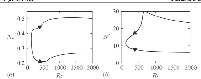
Figure1shows the results in terms of

 

∫

∫

≡

Nu u02 d dy z d dy z, measuring the strength of

the streaks, and

 

∫

∫

′ ≡ +

N (v12 w12) d dy z d dy z, measuring the strength of the asso-ciated spanwisefluctuations( ,v w1 1). These quantities are related to the kinetic energies per unit volume associated with these modes by Eu=Nu 2 and E′ =N′(2Re2). The figure shows that the reduced system captures not only the lower branch states for which it was

Figure 1. Bifurcation diagram showing the lower (downward triangle) and upper (upward triangle) branches of ECS as a function of the Reynolds numberRein terms of (a)Nu=

∫

∫

∫

∫

developed but the upper branch states as well. The two branches connect via a saddle-node bifurcation at Re≈ 136.

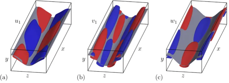
Figure 2 shows streamwise-invariant representations of the lower branch solution at

≈

Re 1500whilefigure3provides insight into the 3D structure of this solution. Figures4and 5 provide analogous representations of the upper branch solution at the same Reynolds number. The lower branch solution is characterized by a smoothly undulating critical layer that is maintained by two nearly circular rolls (figure 2(a)). This structure is supported by fluctuations that concentrate along a critical layer of_O(α_Re)−1 3 _{width (Maslowe 1986,} Wang et al 2007, Hall and Sherwin 2010). Figure 2(b) reveals that thesefluctuations vary rapidly in the direction perpendicular to the critical layer with a much slower variation along it. The 3D representation infigure3confirms these observations and sheds more light on the streamwise dynamics of the lower branch solution: the streamwise velocityfluctuationu1is

concentrated in the regions of strong streamwise-invariant streamfunction ϕ1 (compare

figure2(a) with3(a)) and therefore away from the extrema of the critical layer. In contrast, spanwise fluctuations( ,v w1 1)accumulate at the extrema of the critical layer (figure2(b)), a

Figure 2.The lower branch solution atRe≈1500represented by (a) contours of the streamwise-invariant streamfunctionϕ1and (b) the quantity∥( ,v w1 1)∥L2, a measure of

spanwisefluctuations. In each plot positive (negative) values are indicated in red (blue). The contour plots are superposed on the streak profile shown in black, with the thick solid line representing the critical layeru0=0. All contours are equidistributed.

Figure 3. 3D rendition of the fluctuating flow on the lower branch solution at ≈

Re 1500. The surfaces represented in color correspond to (a) 1max |u|

2 1, (b)

v

max | |

1

2 1, and (c) max |w| 1

2 1, with red (blue) representing positive (negative) values.

consequence of the incompressibility of the fluctuations (equation (12)). At x= 0 (defined arbitrarily as the front section in figure 3), the fluid in the region around the lowest (respectively, highest) point of the critical layer tracks the critical layer from left to right (respectively, right to left); the directions are reversed at locations displaced half a period in the streamwise direction. Figure6shows projections of thefluctuations onto the critical layer

=

u0 0, where they are concentrated. Thefluctuations do not consist of straight,x-oriented, vortices. Rather, their structure is oblique, stretched by the differential forcing iny, and the fluctuation intensity peaks close toz= 0 andz=π 2, where the critical layer departs strongly from the center of the domain y= 0.

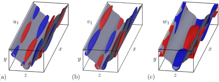
In contrast with the nearly sinusoidal critical-layer profile exhibited by the lower branch solution, the critical layer associated with the upper branch solution is much more strongly deformed from the planey= 0, even approaching at its extrema the top and bottom walls. This change of shape is a signature both of less coherent roll motion and of the splitting of each roll into a bimodal structure (figure 4(a)). This splitting moves the maxima of the streamwise-invariant streamfunction closer to the extrema of the critical layer to support its highly distorted profile. Figures5(a)–(c) show that thefluctuations associated with this state exhibit properties similar to those on the lower branch: the spanwise fluctuations( ,v w1 1) are con-centrated at the extrema of the critical layer with the streamwise velocity fluctuation u1

expelled from these regions. However, thefluctuations also exhibit a bimodal structure with maximum values now located on either side of the critical layer extrema (figure 4(b)). This splitting serves to confine the critical layer in these regions, and leads to strong gradients in

Figure 5.Same asfigure3but for the upper branch solution atRe≈1500. Intersections of thefluctuation contours with the walls aty= ±1that can be observed in (c) are a consequence of the stress-free boundary conditions.

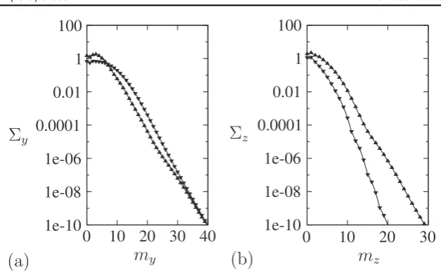
the fluctuation kinetic energy along the critical layer. Differences between the lower and upper branch states are reflected in the Fourier spectra of the associated fluctuation fields (figure7). Thefigure shows the normalized partial sums

⎛

⎝ ⎜ ⎜

⎞

⎠ ⎟ ⎟

∑

Σ =

−

(

)

m

M N S m S m m S m m

( ) 1

2( 1) , 0 ( , ) ( , ) , (18)

y y y

m N

y z y z

2

1

2 2

1 2

z

⎛

⎝ ⎜ ⎜

⎞

⎠ ⎟ ⎟

∑

Σ =

− ₌

m

M N S m m

( ) 1

2( 1) ( , ) , (19)

z z

m M

y z

0 2

1 2

y

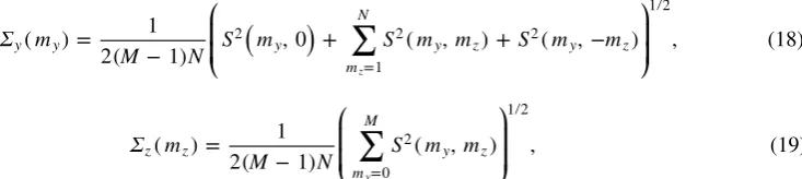
whereS2(my,mz)≡| (v m1 y,mz)|2+ |w m1( y,mz)|2andM(respectivelyN) is the maximum wavenumber in they(respectivelyz) direction. The quantityΣy(my)(respectivelyΣz(mz)) is

therefore related to the energy in modes with wavenumber my (respectively mz) in the y (respectivelyz) direction. The plots indicate that the magnitude of thefluctuations associated with upper branch solutions is larger than that for lower branch solutions. The fact that

Figure 6.Thefluctuations (a)u1, (b)v1and (c)w1along the critical surfaceu0=0. In

solutions along both branches exhibit similar decay inmy(figure7(a)) indicates that the wall-normal structure of the critical layer is similar along both branches. However, the slower decay inmzalong the upper branch indicates the presence of steeper variations inzalong the upper branch, i.e., of solutions that are more strongly localized along the critical layer. These conclusions are confirmed in (x,z) plots of thefluctuations along the critical layer infigure6. The dependence of the upper-branchfluctuations transverse to the critical layer is more abrupt than for the lower branch solution, with strong additional variation along the critical layer near the critical layer extrema at z= 0 and z=π 2. Indeed, the upper-branchfluctuations focus close to the extrema, but plateau away from these points. Comparison of the solutions found here and Nagataʼs solution for PCF (figure7of Jimenezet al2005) reveals substantial similarity: the overall shape of the critical layer, location of thefluctuations and differences between the lower and upper branch states are all quite similar to those in PCF. These common features suggest that our solutions may play a similar role in Waleffe flow to that played by the Nagata solutions in PCF: separating relaminarizing perturbations from turbulence-generating perturbations (lower branch ECS) and capturing the statistical properties of the turbulent state (upper branch ECS). However, our solutions differ from the corresponding PCF solutions in the level of distortion of the critical layer along the upper branch, a difference we attribute to the different nature of the flow and in particular to the more benign stress-free boundary conditions used in the present work.

4. Summary and conclusion

We have described an asymptotic reduction procedure suggested by the lower branch scaling for PCF that appears to apply to parallel shearflows in general. The multiscale asymptotic approach adopted here results in a straightforward derivation of a reduced system of PDEs detailing the interaction between small scalefluctuations and streamwise-invariant structures that serves as a starting point for more detailed investigations. We have used this system to compute both lower and upper branch ECS for Waleffeflow using the Reynolds numberRe

as a homotopy parameter that enabled us to continue the lower branch states into upper branch states. While we do not expect our solutions to be quantitatively accurate for

=

Re O(1), i.e., near the saddle-node, the upper branch states obtained by continuation to large Reare expected to provide an accurate approximation to the upper branch ECS of the full 3D problem, just like the corresponding lower branch states. For these computations the use of Waleffe flow is advantageous since the application of stress-free boundary conditions enables us to employ and refine auniformcomputational grid associated with a trigonometric basis in all coordinate directions.

Our lower branch solutions are qualitatively similar to those for PCF, but the upper branch solutions reveal properties heretofore unknown. These center on the appearance of a bimodal structure in both the streamwise rolls and the associated fluctuations. In an inde-pendent study, a similar asymptotic approach has recently been used to obtain lower branch solutions to PCF (Hall and Sherwin2010, Blackburnet al2013) but no upper branch states were reported.

In future work we will report on the stability properties of these states, including slow streamwise variation, and on their relation to the ECS of the full 3D problem. In addition, new ECS can be identified in the vicinity of the saddle-node captured by the reduced equations and continued to largeRe, where they can be used tofind the corresponding states of the full 3D problem. We mentionfinally that although these equations were derived for a parallel shear flow, the inclusion of slow streamwise variability suggests a systematic path for computing ECS indevelopingflows, including boundary layers.

Acknowledgments

This work was initiated during the 2008 NCAR Geophysical Turbulence Phenomena workshop in Boulder, CO, and developed during the Geophysical Fluid Dynamics Program at the Woods Hole Oceanographic Institution in 2012 (Beaume 2012). The authors gratefully acknowledge support from the National Science Foundation under grants No. DMS-1211953 and 1317596 (CB & EK), No. OCE-0934827 (GPC), and No. OCE-0934737 and DMS-1317666 (KJ). EK also acknowledges support from a Chaire dʼExcellence Pierre de Fermat of the Région Midi-Pyrénées, France.

References

Auerbach D, CvitanovićP, Eckmann J-P, Gunaratne G and Procaccia I 1987 Exploring chaotic motion through periodic rrbitsPhys. Rev. Lett.582387–9

Beaume C 2012 A reduced model for exact coherent states in high Reynolds numbers shearflowsProc. Geophysical Fluid Dynamics Program (Woods Hole Oceanographic Institution)pp 389–412 Beaume C, Chini G P, Julien K and Knobloch E 2014 Reduced description of exact coherent states in

parallel shearflows (arXiv:1407.2980)

Brand E and Gibson J F 2014 A doubly localized equilibrium solution of plane CouetteflowJ. Fluid Mech.750R3

Blackburn H M, Hall P and Sherwin S J 2013 Lower branch equilibria in Couetteflow: the emergence of canonical states for arbitrary shearflowsJ. Fluid Mech.726R2

Chandler G J and Kerswell R R 2013 Invariant recurrent solutions embedded in a turbulent two-dimensional KolmogorovflowJ. Fluid Mech.722554–95

Chini G P, Julien K and Knobloch E 2009 An asymptotically reduced model of turbulent Langmuir circulationGeophys. Astrophys. Fluid Dyn.103179–97

Clever R M and Busse F H 1997 Tertiary and quaternary solutions for plane CouetteflowJ. Fluid Mech.

344137–53

Drazin P and Reid W 1981Hydrodynamic Stability(Cambridge: Cambridge University)

Duguet Y, Willis A P and Kerswell R R 2008 Transition in pipe flow: the saddle structure on the boundary of turbulenceJ. Fluid Mech.613255–74

Giannetti F and Luchini P 2006 Leading-edge receptivity by adjoint methodsJ. Fluid Mech.54721–53 Gibson J F, Halcrow J and CvitanovićP 2008 Visualizing the geometry of state space in plane Couette

flowJ. Fluid Mech.611107–30

Gibson J F and Brand E 2014 Spanwise-localized solutions of planar shearflowsJ Fluid Mech.745 25–61

Halcrow J, Gibson J F, CvitanovićP and Viswanath D 2009 Heteroclinic connections in plane Couette flowJ. Fluid Mech.621365–76

Hall P and Sherwin S 2010 Streamwise vortices in shearflows: harbingers of transition and the skeleton of coherent structuresJ. Fluid Mech.661178–205

Jimenez J, Kawahara G, Simens M P, Nagata M and Shiba M 2005 Characterization of near-wall turbulence in terms of equilibrium and‘bursting’solutionsPhys. Fluids17015105

Kawahara G, Uhlmann M and van Veen L 2012 The significance of simple invariant solutions in turbulentflowsAnnu. Rev. Fluid Mech.44203–25

Khapko T, Duguet Y, Kreilos T, Schlatter P, Eckhardt B and Henningson D S 2014 Complexity of localised coherent structures in a boundary layerflowEur. Phys. J.E11232–45

Lucas D and Kerswell R R 2014a Spatiotemporal dynamics in 2D Kolmogorovflow over large domains

J. Fluid Mech.750518–54

Lucas D and Kerswell R R 2014b Recurrentflow analysis in spatiotemporally chaotic 2D Kolmogorov flow (arXiv:1406.1820)

Maslowe S A 1986 Critical layers in shearflowsAnnu. Rev. Fluid Mech.18405–32

Nagata M 1990 Three-dimensionalfinite-amplitude solutions in plane Couetteflow: bifurcation from infinityJ. Fluid Mech.217519–27

Schneider T M, Gibson J F, Lagha M, de Lillo F and Eckhardt B 2008 Laminar-turbulent boundary in plane CouetteflowPhys. Rev.E78037301

Schneider T M, Gibson J F and Burke J 2010 Snakes and ladders: localized solutions of plane Couette flowPhys. Rev. Lett.104104501

Skufca J D, Yorke J A and Eckhardt B 2006 Edge of chaos in parallel shearflowPhys. Rev. Lett.96 174101

Waleffe F 1997 On a self-sustaining process in shearflowsPhys. Fluids9883–900