White Rose Research Online [email protected]
Universities of Leeds, Sheffield and York
http://eprints.whiterose.ac.uk/
This is the author’s post-print version of an article published in Transportmetrica
White Rose Research Online URL for this paper:
http://eprints.whiterose.ac.uk/id/eprint/77994
Published article:
Balijepalli, NC, Ngoduy, D., and Watling, DP, (2013)The Two-regime Transmission Model for Network Loading in Dynamic Traffic Assignment.
Transportmetrica. 1 - 22. ISSN 1812-8602
The Two-regime Transmission Model for Network Loading in Dynamic Traffic Assignment Problems
Balijepalli, N.C., Ngoduy, D. and Watling, D.P1.
Institute for Transport Studies, University of Leeds, England LS2 9JT
Dynamic Network Loading (DNL) model is concerned with moving traffic in space and time along road network links in Dynamic Traffic Assignment (DTA) models. DNL models strive to build in traffic realism such as modelling transient queues and spillback to upstream links, yet they need to remain computable. Most models in the literature are skewed towards either realism or computability and thus leave a wide scope for further research in arriving at a balanced model. This research proposes a new DNL model called the Two-regime Transmission Model (TTM) based on widely accepted first order traffic flow theory. The TTM is aimed to be quick and accurate enough for planning purposes, when embedded into the framework of a DTA. The TTM considers the time dependent density states of network links over two regimes viz., free-flowing and congested regimes, and dynamically models the time dependent queue length, but without the need to break the link into cells. This article sets out the theoretical background necessary for developing the TTM and it also illustrates the principles with the help of a simple network serving a single OD pair. Although the numerical tests are only preliminary indicators, the TTM has been found to produce promising results, for example producing results that are apparently closer than the Cell Transmission Model to predicting the dissipation and formation of a queue in a homogeneous link for the same level of time discretisation. We believe that our work establishes TTM as a candidate worthy of future exploration, especially for representing plausible, first-order traffic dynamics within a dynamic user equilibrium model with a lower number of variables/side-constraints than the Cell Transmission Model.
Keywords: Cell Transmission Model (CTM), Dynamic Traffic Assignment, Two-regime Transmission Model (TTM), Dynamic Network Loading (DNL), LWR model.
1. INTRODUCTION
Traffic network equilibrium models are used in a wide range of operational and planning applications, from real-time information/control to medium-to-long term forecasting. In planning approaches, they are commonly used to estimate the costs and benefits associated with planned policies and measuressuch as new infrastructure, congestion pricing or new housing/retail developmentsand are often used to forecast the impacts on and of future travel demand patterns over time horizons up to twenty years ahead. Clearly in such a planning context, there exists considerable uncertainty in the future origin-destination demands that will actually occur. Thus, planning problems such as these are distinctive from online applications, since in the latter we have much higher quality data, as we may monitor and estimate to a reasonable accuracy the demands for that particular day. In planning applications, on the other hand, we accept a considerable degree of uncertainty in forecasting future demand levels. The point of this remark is that these two quite different contexts may in turn place different requirements on the traffic flow representation in our model. That is to say, in a planning context we may accept a relatively „coarse‟ representation of congestion phenomena, as we are not tracking the movement of demands actually monitored on a
1
specific day, but of OD demands that represent broad estimates of likely future travel patterns. The focus of the present paper is specifically on these longer-term, planning contexts.
For many years, network equilibrium analysis developed around the „static‟ model, based on steady state flows and time-independent relationships between link travel time and link flow (Sheffi, 1985). However, it is now a rather widely held belief that such relationships are too coarse even for planning applications: they lead to systematic bias at the broad level; it is not just a question of „detail‟. In their place we have seen the development of dynamic network equilibrium models (as reviewed, for example, in Peeta and Ziliaskopoulos, 2001), whereby the deficiencies of static models are addressed by propagating flows in time as well as space, restricting flows by capacity, allowing travel times and traveller route choices to vary with time during the modelled period, and requiring that the traffic is loaded in such a way that the entry/exit flows and travel times are internally consistent.
One can envisage such dynamic equilibrium models as comprising an „equilibration‟ component whereby departure-time-dependent path in-flow rates are determined, and a dynamic network loading model which „determines,… over a fixed time period, link cumulative arrival/departure curves (hence time dependent link/path travel times) corresponding to a given set of temporal path flow rates‟ (Nie et al 2008). As this definition indicates, our interest during network loading is principally in what happens to traffic as it enters and exits a link (this is sufficient to infer link travel time profiles, assuming FIFO to hold at the link level), not in what happens within the link. Such an observation no doubt motivated the development of approaches to this problem based on analytical properties of the prevailing state of the link as a wholesuch as its in-flow, out-flow or densityrather than considering the details of what happens within the link. These notably include approaches based on exit functions (e.g. Merchant and Nemhauser, 1978; Smith, 1983), where the flow exiting a link at any time instant is assumed to be a time-dependent function of the current link state, and those based on travel time functions (e.g. Friesz et al, 1993, Astarita, 1996, Xu et al 1999), where instead the travel time to traverse a link for a vehicle entering at any time instant is assumed to be a time-dependent function of the current link state.
As experience with using such „whole-link‟ approaches has grown, so has the understanding of the „desirable properties‟ with which particular forms of them imbue both the network loading (Xu et al, 1999; Carey, 2004a, 2004b) and the equilibrium solution as a whole (Szeto and Lo, 2006). For example, if we adopt a travel time function approach then the most general known conditions to ensure FIFO require either the function to be linear or a bound to be satisfied on the rate of change of the in-flow rate, otherwise FIFO may be violated (Xu et al, 1999). Carey (2004a) broadened the link-level considerations to uniqueness, continuity, causality and time-flow consistency, subsequently noting that approaches based on exit-flow functions violate causality (Carey, 2004b). As such limitations have been identified in the whole-link approaches, so has more attention been paid to the more general plausibility of the physical traffic behaviour underlying the whole-link approaches within the link. As a result there has been a discernible trend in the dynamic traffic assignment literature away from „whole-link‟ approaches, toward those that explicitly consider the dynamics of flow within the link, and especially the Cell Transmission Model (CTM) due to Daganzo (1994, 1995).
that cell‟s current density and in-flow and ii) the potential for the „receiving‟ cell to receive in-flow from the „sending‟ cell, given the receiving cell‟s current density. The appeal of the model is particularly that in the continuous limit of space and time, it converges to the kinematic wave (LWR) model of Lighthill and Witham (1955) and Richards (1956), based on an analogy between traffic flow and certain types of wave motion in fluids. The LWR model is able to replicate realistic phenomena of traffic flow observed along a link, such as „waves‟, and for this reason has established itself as a standard by which to judge the reasonableness of dynamic congestion relationships. In this respect, Nie & Zhang (2005) studied the performance of several „whole-link approaches‟ against the standard of an LWR model (estimated in discretised form by the CTM). They found that, relative to LWR, the travel time function models they tested tended to overestimate travel times, and that exit function models tended to over-estimate (under-estimate) travel times when the link in-flow rate decreased (increased) suddenly.
Moreover, it should be noted that importantly for dynamic network modelling, such „physical queuing‟ approaches are not only appealing for modelling link traversal time, but also give a realistic representation of queue spillback to upstream links (Gentile et al 2007). Such a feature is potentially of increasing importance in a planning context in many developed and developing cities of the world, where any strong future growth in demand (without corresponding increase in capacity) may lead to many parts of the network operating in such regimes.
Thus, the state-of-the-art in dynamic traffic assignment leaves us in a position where, in order to obtain plausible link traffic flow dynamics, to reflect spillback to upstream links, and to obtain reasonable travel times (according to the LWR standard), then we are given the obvious choice of selecting the CTM, known to be a discretised form of LWR. Yet this means that, counter to our earlier discussion on the role of such models in a planning context, we end up modelling in great detail the within-link traffic flow dynamics and wave propagation of demands which (in such a longer term planning context) are highly uncertain and at best represent broad estimates. Moreover, the choice to adopt CTM is not without its computational overheads. As Nie & Zhang (2005) note, if we just consider the issue of dynamic network loading (of given route in-flow profiles) then the computational time for the CTM is directly proportional to the number of cells, and hence the computational efficiency is inversely proportional to the accuracy (in recovering the LWR). Thus the choice of discretisation level effectively means a choice/compromise between computational efficiency and the level of agreement with the LWR model. If we then consider the wider issue of how the model may be integrated within a dynamic network equilibrium framework, then we are faced with further computational issues: if the CTM is specified as a set of side constraints as suggested by Peeta & Ziliaskopoulos (2001) then the number of constraints grows with the fineness of the discretisation, whereas if we represent it using a route-based mapping as in Lo and Szeto (2002), then we are led down a path of route enumeration with all the computational difficulties that it is known to bring. As Bar-Gera (2005) notes, the „computational requirements reduce the attractiveness of this model for large-scale long duration applications‟.
potentially provides computational advantages (e.g. in terms of the number of variables required as side constraints in solving a dynamic user equilibrium problem). Moreover, the intention is that this parsimony is not only in terms of spatial discretisation but also potentially in the level of temporal discretisation, an issue that we explore numerically. Specifically our test of „consistency with LWR‟ will not be in terms of the theoretical limit as the time-increments approach zero, but in the practical limit of consistency with its discretised CTM version at the same level of temporal discretisation. This also allows us to explore how the degree of conformity with the LWR model varies as the discrete time intervals become larger in duration, an issue that has more relevance for algorithm design than the limit of infinitesimal intervals. While the model we propose may not be appropriate in all the cases for which CTM issuch as modelling incidents or real-time control measuresour aim will be that for most medium-term planning applications it will be sufficient, for reasons that we explain below. The structure of the paper is as follows. Section 2 describes the mathematical derivation of the link models, comparing the elements of the new model with existing approaches, and provides a specification of a practical computational algorithm. Section 3 reports the findings of illustrative numerical experiments conducted on a simple network previously studied in this journal series. The experiments specifically focus on comparisons between the new model and the CTM in a dynamic network loading context (i.e. when route in-flow profiles are given) when queue builds up and dissipates, and on the impact of different levels of temporal discretisation. Additionally, by a slight amendment of the network, a simple route choice problem is created, allowing a numerical exploration to be made of the existence of dynamic user equilibrium solutions with the new model embedded. While the numerical experiments are limited to small-scale examples definitive conclusions cannot be drawn, but in section 4 we draw together the suggestive features from these experiments to be pursued in further research and testing.
2. MODEL DEVELOPMENT
The aim of our approach will be to capture the “essential elements” of the LWR model in a simplified dynamic congestion relationship, which does not require the cell-level disaggregation of the CTM. Given our interest in dynamic traffic assignment for planning applications, our interest will be specifically in examining recurrent congestion patterns, assuming that congestion is due to fixed, predictable bottleneck locations on the road network. Such bottlenecks will typically occur where physical changes to the road appear, such as lane drops, merges, intersections, traffic signal controls, steep gradients, sharp bends, or possibly „frictional‟ distractions due to roadside activity. By coding the network such that nodes are defined at any such fixed bottleneck location, then we may make the assumption that congestion may only begin to form at the downstream end of a link. Such an assumption would not be suitable for analysing moving bottlenecks, neither for representing incidents or the effect of rain/snow which may cause bottlenecks to occur at unpredictable locations; in such cases the CTM would remain the appropriate choice. However, we believe that there exists a wide range of planning applications for which a fixed bottleneck assumption would be appropriate. In the ensuing section we shall describe the method by which traffic is propagated along a link. This is the core part of this paper where we describe a method to model the propagation of the queue in a link based on the inflow and outflow at the upstream and downstream node, respectively.
dependent on the total density along the link but independent of the destination. To apply the LWR model for each destination-oriented density, it is straightforward to show that the following equation is satisfied:
0
k q
t x
(1)
Let V V k x te
,
denote the mean speed as a function of density (the so-called speed-density relationship), then by definition qq k x te
,
kV k x te
,
(which incorporates the flow-density relationship). In both cases, we assume relationships that are independent of time t and location x, in accordance with an assumption of a homogeneous link. Moreover, in the case of the flow-density relationship, for simplicity of exposition we shall focus in the present paper on the particular case of a triangular flow-density relationship (even though we believe the method to be readily extensible to general flow-density relationships).CTM (Daganzo, 1994, 1995) approximates the LWR model by dividing the link into cells of equal length dx and dividing time into time steps of equal duration dt. In CTM, our freedom to vary the cell length and time step is constrained by the Courant–Friedrichs–Lewy (CFL) condition that they must satisfy dxV dt0 , where V0 is the free flow speed. The CFL
condition is used to guarantee that vehicles will not travel further than the length of the cell within a time step, so as the numerical stability and errors do not grow unbounded (see Sod, 1985). Rather obviously, the accuracy of approximation of the CTM to the LWR model is a function of the number of cells/time steps: to accurately reflect the qualitative behaviour of the LWR we may need a potentially fine level of discretisation, which could be computationally intensive. As Nie and Zhang (2005) express it, since the computational time in CTM is directly proportional to the number of cells, and then we can say that the computational efficiency is inversely proportional to the accuracy. To this end, we will propose in the rest of this section a new model, which demands less computation than CTM but which still captures the attractive feature of the LWR model in representing how a traffic jam forms and dissipates along a link.
First of all, we apply the principle proposed by Newell (1993) to equation (1): that is, the cumulative flow along a characteristic wave changes at a constant rate either in free-flow or in congested conditions. Accordingly, the flow in each traffic condition is computed as:
0
0
( , ) if traffic is in free-flow condition ,
( , ) if traffic is in congested condition
in
c out
c x q x t q t
V q x t
L x q x t q t
(2)
whereq x t0( , )and q x tc( , )are the flows in the free-flow and congested condition. qin and qout
are the inflow and outflow at the upstream and downstream node of the considered link. c denotes the wave speed in the congested condition. Note that in the free-flow condition, the disturbances travel downstream, whereas in the congested condition the disturbances travel upstream, hencec 0. wc is the slope of the congested branch of the flow-density
relationship. From the fundamental diagram we obtain the density k x t
, qe1
q x t
,
, where here 1(.)
e
Now, as noted earlier, we shall assume that the link is homogeneous and the actual bottleneck is at the downstream node. If there are other constraints within the considered link such as lane-drops, we should split the link into several sub-links with constant capacity and corresponding sub-nodes between them. Furthermore, we also assume that traffic along a link is characterized by two regimes (i.e. either free-flow or congested), which are then considered in two cases as defined below. Due to the importance of this feature in our modeling approach, we have named it the Two-regime Transmission Model, or TTM for short. The idea of modelling a link as two traffic regimes has been applied in Bliemer (2007). However, Bliemer (2007) did not model the spatial and time dynamics of the density or flow along the link in detail, whereas our model allows for describing the dynamics of density along the link. Depending on how traffic flows into and flows out of the link, the length of each regime is determined. Instead of describing the dynamics of traffic on links through many cells with an equal length as in the CTM, TTM takes into account the changes in the density between each regime and the propagation wave speeds of each regime. With these assumptions, we are only interested in the jam formation and the propagation of the upfront jam under a certain boundary condition (when and where a traffic jam occurs). To this end, we will show that the traffic dynamics at a certain location in the link can be determined by the upstream boundary conditions in the free-flow situations and/or by the downstream boundary conditions in the congested situations.
Before continuing to present our approach, it is relevant at this stage to contrast our TTM approach with recent work by Yperman et al (2006), since (on the surface) there are some similarities. In a similar spirit to our approach, they combined CTM with Newell‟s (1993) cumulative curves and treated each complete link as if it were a single cell, giving their resulting model the name Link Transmission Model (LTM). As the link is considered as a whole entity, the computational effort required to implement the LTM is substantially less than that of the CTM. The flow propagation in LTM is based on Newell‟s cumulative flow curves applied at the entry/exit of each link, with node models used to calculate the transition flows which are based on conservation of flow between the incoming and outgoing flows. Sending/receiving flows together with transition flows and other flow constraints form the basis for updating the cumulative flows at the link boundaries. However, our TTM approach departs from the LTM approach in important ways. In particular, TTM assumes that the link is divided into two parts (congested and free-flow regimes) and models the queue length dynamically based on shockwave theory. This means that the TTM is able to capture the queue dynamics both in (horizontal) space and time. In this respect TTM takes a completely different course to that of LTM although both models have Newell‟s theory (and hence the LWR model) as a common starting point.
Returning, then to the definition of our TTM approach, we now go on to consider the different cases that may arise:
Case 1: Traffic starts loading into the link with free flow speed V0. In this case, the length of
the first regime (L1) is increased up to the whole length of the link (L), that is when vehicles
reach the downstream node (See Figure 1). The time dynamics of L1 is given by:
1 0
dL V
dt (3)
or
1
1 min , 1 0
t t
L L L V dt (4)
Figure 1 Traffic loading
According to equation (2), the flow along the link is:
0 1
0
( , ) ( , ) in , t
x
q x t q x t q t x L V
(5)
The density is computed from the free-flow branch of the fundamental diagram. Equation (5) clearly indicates that if there are no downstream constraints, the traffic states along the link are entirely determined by the inflow from the upstream node. From equation (5) the density
at location x and time instant t is
1 1 0, e in( x) ,
k x t q q t x L
V
and k x t
, 0, x L1Case 2: Vehicles have reached the downstream node and a queue starts to build up. In this case the queue will propagate upstream with the shock wave speed b as described in Figure 2. It is worth noticing in this figure that there are multiple values of density along the link when the traffic inflow from the upstream node and traffic outflow at the downstream node frequently fluctuates. Mathematically, it can be seen from equation (2) we can compute the
density in the free-flow regime at location x and time t by
10
, e in( x)
k x t q q t V
and the
density in the congested regime at location x and time t by
, e1 out( )c L x k x t q q t
. Note
that bdescribes the slope of the line connecting a point in the free-flow branch with a point
in the congested branch of the density-flow relationship; it should not be confused with c
which is the slope of the congested branch of the flow-density relationship. In principle, the length of the congested regime is dependent on the propagation speeds of the shock wave generated by the control settings at the downstream node and the demand coming from the upstream node. To compute the shock-wave speed, we apply the Rankie-Hugoniot (RH) condition for the boundary between the free-flow and congested regime. In principle, the RH condition is used to relate the behaviour of shock waves travelling to the prevailing flow. We obtain the shock-wave speed at the boundary as below:
jump in flow
, jump in densityb b
b
b b
q t q t t
k t k t
(6)
where qband qbdenote, respectively, the flow at the right and left interface between the free-flow and congested regime. kband kbare the density at the right and left interface between
V0
De
nsit
y
L1 L2=L-L1
the free-flow and congested regime, which are computed from the fundamental diagram given the flow qband qb, respectively: 1
1
( ) , ( )
b e b b e b
k t q q t k t q q t . From equation (2) we obtain:
2
1
0
,
b out b in
c
L t L t
q t q t q t q t
V (7)
From equation (6), we obtain the dynamic equation for the length of the congested regime as:
2 b ,
dL dt (8)
or
1 1 1
2 min , 2 , 1 max 0, 2
t t t t
b
L L L dt L LL (9)
From equation (8), ifb 0, that is qb
t qb
t
, the shock is moving upstream, the length of
the congested regime is increased, whereas if b 0, that is qb
t qb
t
, the shock is dissipating downstream, the length of the congested regime is decreased. Nevertheless, if
0
b
(qb
t qb
t
) the length of the congested regime is unchanged (stationary).
Figure 2 Queue propagation
Equation (8) means that the length of the congested regime is controlled by the total flow rate that wishes to enter the queue (calculated from the inflow at the upstream node) and the total flow rate that has entered the queue (calculated from the outflow at the downstream node). Given the inflow at the upstream node, if there is any constraint at the downstream node (e.g. red light or less capacity of the outgoing links), the queue is growing; otherwise, it is dissipating.
According to equation (2), the flow along the link is:
t 0 1 0 t 1( , ) if x L ,
( , ) if x>L
in
c out
c x q x t q t
V q x t
L x q x t q t
(10)
and the density is computed from the free-flow branch of the fundamental diagram if t 1
xL , and from the congested branch otherwise. That means based on equation (10), we can
b
De
nsit
y
L1 L2
calculate the density for each traffic condition given the length of the congested part (or free-flow part) and the infree-flow and outfree-flow profiles at the upstream and downstream node.
Limitations of the TTM:
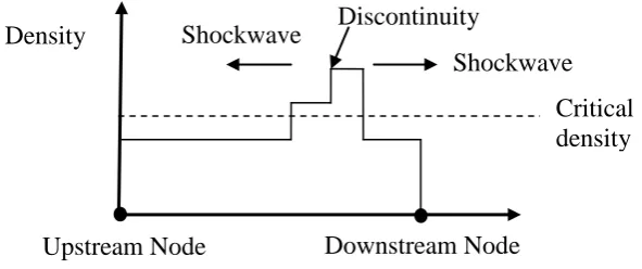
[image:10.595.120.416.272.406.2]TTM assumes that congestion occurs only at the downstream end of the link. In other words, the link should have homogeneous capacity. If there is a lane drop somewhere along a road link, then the link needs to be divided into two sub-links before applying the TTM. Aside from the above, it is also possible that within a congested regime on a given road link there can exist situations with more than one density. Multiple densities within a congested regime are known as discontinuity in densities. The TTM can deal with the situation of one shockwave and a discontinuity in density such as the one shown in Figure 3 below, for example.
Figure 3 One Shockwave and a Discontinuity in Density
However, TTM is not an appropriate choice to deal with a double shockwave shown in Figure 4 arising due to a temporary bottleneck such as an incident occurring along the link.
Figure 4 Two Shockwaves and a Discontinuity in Density
We also clarify that the model cannot deal with advanced traffic flow modelling features such as moving bottlenecks. Finally, the purpose of the model as described in the introduction, is to help the planning applications in the medium term situation and hence TTM is not suitable to deal with short t
rm control such as incident management.
Critical density Discontinuity
Shockwave Density
Downstream Node Upstream Node
Critical density Shockwave
Density
Downstream Node Upstream Node
Discontinuity
[image:10.595.116.412.463.587.2]3. NUMERICAL STUDIES
3.1. Network Description
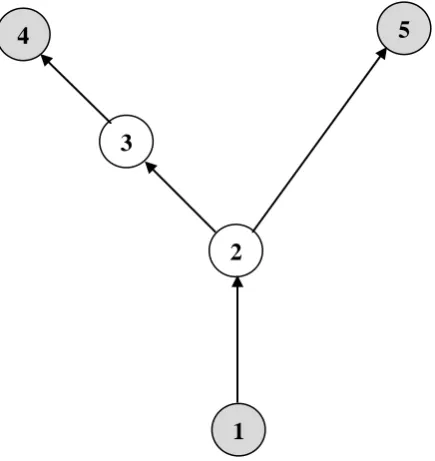
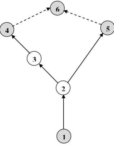
Our numerical investigation and illustration of the principles described in this paper is based on a simple Y-shaped network, which is similar to the network used by Szeto and Lo (2006). In particular, the network connects two destinations to one origin by one route each, as shown in Figure 5. We shall refer to route 1 as that travelling to node 4, and route 2 as that travelling to node 5. While links (1,2) and (2,3) have equal capacity, link (3,4) is assumed to have half the capacity of link (1,2) or (2,3). The lower capacity of link (3,4) simulates the effect of a lane-drop and will cause congestion leading to queuing and potential spillback to upstream links, depending on the demand profile. Route 2, on the other hand, consists of two links which have equal capacity. The particular characteristics of the network links are summarised in Table 1. The triangular flow-density relationship we have assumed can be constructed from the values specified in the Table. This relationship differs a little in shape from that assumed by Szeto & Lo (2006) in particular in our assumption of a shock wave speed which is rather less than the free flow speed, since we feel the value we have assumed is better supported by reported empirical evidence.
[image:11.595.187.405.360.591.2]
Figure 5 Experimental Network
4 5
3
2
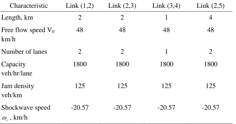
Table 1 Network Link Characteristics
Characteristic Link (1,2) Link (2,3) Link (3,4) Link (2,5)
Length, km 2 2 1 4
Free flow speed V0 km/h
48 48 48 48
Number of lanes 2 2 1 2
Capacity veh/hr/lane
1800 1800 1800 1800
Jam density veh/km
125 125 125 125
Shockwave speed
c
, km/h
-20.57 -20.57 -20.57 -20.57
The modelling is carried out over a total period of 900 seconds. We have considered a demand profile varying over time. Let represent the traffic demand (veh/hr) between OD pair k at time t. The demand profile for OD pairs (1,4) and (1,5) is specified as below:
and
.
Note that the demand ceases much earlier than the extent of simulation horizon which is intended to allow all the vehicles on the network to reach their destinations before the end of the simulation period. Also note that the demand D(1,4) on route 1 is expected to create congestion on link (2,3) because the exit capacity of the link is limited by the capacity of the link (3,4) which has only one lane. However, route 2 is not expected to be congested as the demand D(1,5) is well below the capacity of the links on the route.
3.2. Example 1: Performance of TTM and CTM
Both TTM and CTM are simulated with different time steps dt=1sec. and dt=10sec. Note that in CTM, the link is divided into cells with equal length dx=V0dt, where V0 is the free speed
CTM in reproducing the formation and dissipation of the queue, we use a fine mesh CTM (dt=1sec) as our practical approximation to the analytical LWR solution. The formation and dissipation of the queue along link (2,3) is plotted at some time instants as in Figures 8 and 9. It is seen that, given a much larger time step (dt=10sec.), the density profiles predicted by TTM are closer to the fine-mesh-estimated LWR profiles (i.e. CTM with dt=1sec.) than are the profiles predicted by CTM with dt=10sec.
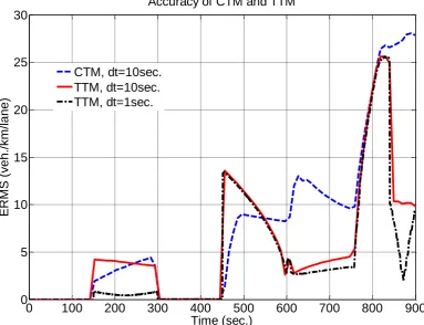
The deviations of numerical errors by TTM and CTM for different time steps, in comparison with the “exact” (fine-mesh CTM) solution, are then studied using the so-called Euclidian root mean square (ERMS) error norm as:
( ) Meanx sim( , ) exact( , ) ,
E t k x t k x t (11)
where E t( ) is the Euclidian error norm. Here, Meanxdenotes the mean operator over all
locations; ksim( , )x t is the density computed by the simulation (TTM or CTM) for a given time
step; and kexact( , )x t is the density computed by the fine-mesh CTM (dt=1sec). Figure 10 shows that the ERMS of TTM for dt=1sec is slightly smaller than TTM for dt=10sec during the traffic loading situation (Case 1) and during the queue dissipation (Case 2) and is rather comparable during the rest of the simulation time. However, the ERMS of TTM for both dt=1sec and dt=10sec are both smaller than that of CTM during most simulation times. This is because an increased time step requires a larger cell length in the CTM, which increases the smoothing effect in CTM more significantly than in TTM. It is worth emphasising here again that TTM is different from CTM in its approach to spatial discretisation, particularly as the temporal discretisation is varied. When the time step is reduced, the cell length in the CTM must be reduced simultaneously in order to satisfy the CFL condition, and thereby to converge in the continuous limit to LWR. However, this is not the case in TTM since even when the time step is reduced, there are still two regimes being modelled (in either Case 1 or Case 2) so that TTM does not spatially converge to LWR. That explains why when the time step is reduced to 1sec, the accuracy of TTM does not improve significantly. Let us take a closer look at Figure 10, we find that before t=150sec, link (2,3) is empty so obviously ERMS=0. Between t=150-300sec, traffic starts loading into link (2,3) as in Case 1 and ERMS is similar between TTM and CTM. Between t=300-450sec, that is when the demand is increased, all vehicles have reached node 3 and link (2,3) is operating under the capacity. In this condition, the density is equal to critical density so ERMS=0. Between t=450-900sec, the queue starts to build up and dissipate along link (2,3).
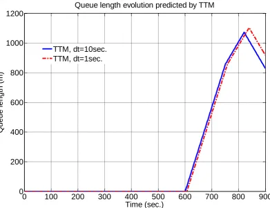
Figure 11 describes the evolution of the queue length (that is the dynamics of L2) predicted by
TTM (using dt=1sec and dt=10sec). It is concluded from this figure that the evolution of the queue length in TTM is not influenced significantly by the length of the time step, at least in this example. Thus, although not its only purpose, we have the opportunity to use a coarser scale temporal resolution for TTM in order to significantly reduce the number of variables that need to be considered in a dynamic user equilibrium context (e.g. as side constraints or as a directly computed loading), which would be expected to offer significant computational advantages. Clearly the embedding of TTM within a dynamic user equilibrium algorithm is an area that would merit further research.
using a time increment of dt=10sec for both then TTM required 6 seconds whereas CTM required 16 seconds. However, the example considered suggests that we would need a smaller time increment for CTM (and hence a longer computational time) in order to predict the dynamics of the horizontal queue as accurately as TTM does, so our initial work suggests that the computational advantage (purely for network loading) of TTM over CTM for a prescribed level of accuracy may be even greater than that the comparison at a common time increment suggests. Nevertheless, the example network is small so more extensive experiments need to be carried out to confirm our findings, which will be left to our future research.
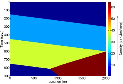
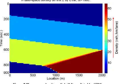
Figure 7 Phase-space density on link (2,3) predicted by CTM
Figure 9 Queue dissipation at node 3 and moving downstream on link (2,3)
Figure 10 Performance of TTM and CTM in reproducing the formation and dissipation of queue on link (2,3).
0 100 200 300 400 500 600 700 800 900
0 5 10 15 20 25 30
Time (sec.)
E
RM
S
(
ve
h
./
km
/la
n
e
)
Accuracy of CTM and TTM
[image:16.595.103.487.409.703.2]Figure 11 The dynamics of queue on link (2,3) predicted by TTM.
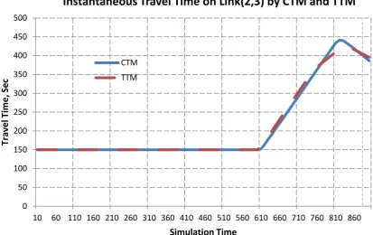
In order to compare the two models further, firstly we compare the instantaneous travel time by TTM and CTM (dt = 1sec) in Figure 12. The model is a flow/density-based model in that it represents the flow/density at each time along the length of a road link. We have used the flow-density relationship (as defined by the parameters set out in Table 1) to arrive at the speed associated with a given set of flow-density values. Typically, if the density is less than or equal to the critical density then that part of the link operates at free flow speed, otherwise the speed will be equal to the fraction of flow divided by the density. In case of TTM, we know the lengths of free flow and congested regimes, dividing the length of either free flow or congested regime by applicable speed gives the travel time within that regime. Summing the free flow time and congested time gives the total travel time. The above method is equally applicable for CTM as well. In CTM, the lengths of cells are fixed and are a known quantity. Following through similar steps as explained above will get us to the required travel time. From the figure we note that the travel time by TTM compares well with that by CTM which is intuitively reasonable to expect given the similarity of density profiles between the two methods as shown earlier in Figures 6 & 7.
0 100 200 300 400 500 600 700 800 900
0 200 400 600 800 1000 1200
Time (sec.)
Q
u
e
u
e
le
n
g
th
(
m
)
Queue length evolution predicted by TTM
Figure 12 Instantaneous Travel Time on Link(2,3) by CTM and TTM
Dynamic traffic assignment models will need the actual travel time as experienced by the drivers on a road link rather than the instantaneous travel time. Therefore, we also compare the experienced travel times by TTM and CTM (dt =1sec) in Figure 13. The experienced travel times have been worked out based on the method of cumulative curves (Long et al 2010) as set out below.
Let be the cumulative inflow to a road link up to the time t, such that
and be the cumulative outflow given by . For any vehicle the entry time to a link is given by the inverse of cumulative inflow curve. Similarly, the exit time from the link is given by the inverse of cumulative outflow curve. Assuming FIFO to hold on the link, the difference between the exit time and entry time to the link gives the experienced link travel time. Thus the travel time (t) at time t can be written as
. Figure 13 indicates that the experienced travel times by TTM and CTM are almost identical to one another as any minor differences between the two were nullified due to the aggregation involved with the method of cumulative curves. It is noted that the illustration of DTA in the ensuing section has been based on experienced travel times and not the instantaneous travel times.
0 50 100 150 200 250 300 350 400 450 500
10 60 110 160 210 260 310 360 410 460 510 560 610 660 710 760 810 860
Tr
av
el
T
ime,
Se
c
Simulation Time
Instantaneous Travel Time on Link(2,3) by CTM and TTM
Figure 13 Experienced Travel Time on Link(2,3) by CTM and TTM
3.3. Example 2: Dynamic Traffic Assignment with TTM
Figure 14 Modified experimental Network
In section 3.2 we explored TTM in a dynamic network loading context, but in fact with a slight modification to our example network we are also able to study a simple example of dynamic user equilibrium. The modification involves merging the two original destination nodes (4 and 5) together, using dummy links with infinite capacity and zero travel time to join
0 50 100 150 200 250 300 350 400 450 500
10 30 50 70 90 110 130 150 170 190 210 230 250 270 290 310 330 350 370 390 410 430 450
Tr
av
e
l t
im
e
, se
c
'n'th vehicle that had entered the link
Experienced Travel Time on Link(2,3)
CTM TTM
4 5
3
2
them to a single common destination node 6, as illustrated in Figure 14. After this amendment, we have a network with one OD pair served by two routes. We assume that all the characteristics of the links described earlier remained unchanged. In order for the route choice to kick in, the demand profile is also slightly revised by unifying the two previously separate destination-based demands as below:
.
The above alterations to the network and the demand profile mean that in each departure period drivers have now have a choice to select route 1 or 2; it is assumed that their objective is purely to minimise their own (predictive) travel time. We suppose that drivers perceive differences in average travel time over the three major time periods (of duration 300 seconds each) over which the demands are specified, so that route choice varies by major departure time period and the travel times experienced are the averages over the major period considered (a finer discretisation of dt=10 secs used in dynamic network loading). A dynamic user equilibrium state is said to have been reached when no driver in any given major departure period is able to unilaterally switch their route in order to reduce their travel time.
The purpose of the experiment we describe is two-fold. Firstly we wish to examine whether the TTM behaves in a systematic, plausible manner as the route fractions by time period are altered. Secondly, we wish to explore the existence (and multiplicity) of dynamic user equilibria; as Szeto and Lo (2006) discuss, such issues even as existence of equilibria cannot be taken for granted when we use more complex, physically realistic traffic models such as those considered in the present paper. Due to the structure of our example network which has a single origin node, and due to the fact that by construction TTM is consistent with both causality and FIFO, we are able to solve for dynamic user equilibrium in a special way. In this case, we load only traffic from the first departure period, setting the demands for later periods to be zero, and compute an equilibrium state for this period in isolation. Given the equilibrium flow proportions computed for period 1, this period can then be loaded, and we then move on to period 2, assuming period 3 demands to be zero, and compute an equilibrium state for period 2, given that period 1 has already equilibrated; and so on. This incremental method will give us a dynamic user equilibrium solution in our network, as demands from later time periods cannot affect the travel times from earlier periods.
In practice, then, we achieve both of our objectives (of exploring the impact of differing route choice fractions and of finding dynamic user equilibria) by the following method. Let us denote the (unknown) proportion of drivers from major departure period k that choose route 1 by k and that choose route 2 by k, for k =1,2,3. Clearly , as we have only two routes. The aim is to find the values of these fractions for each departure period for which the resulting route travel times on used routes are equal and minimal. Our „incremental‟ method then proceeds as described in the following steps.
i. Initialise the considered departure period to be period k = 1.
ii. For all periods before period k, set the fractions of drivers on the two routes to the already-computed equilibrium solution for that period (conditional on other periods having been loaded). For all periods after period k, set the origin-destination demand to zero.
traffic to reach its destination in order to obtain the route travel times for the given route fractions for period k.
iv. In locations where equilibrium conditions are close to being met, perform a finer search over route choice fractions for period k to more accurately compute the equilibrium solution for period k, conditional on other periods having been loaded. v. If k < 3, increment the value of k by 1 and return to repeat steps ii. – iv. until we reach
the end of the modelled period.
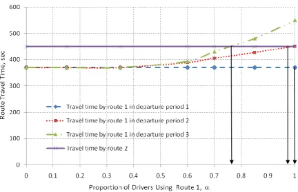
By following step iii., we compute route travel times for each period k over a given range of route choice proportions for that period, conditional on earlier periods already having been loaded according to their equilibrium proportions. Figure 15 illustrates the results of these experiments for the example network. The way to interpret Figure 15 is as follows: choose one of the three departure periods to analyse, let us say period 2. Then the horizontal axis represents different pre-defined route choice proportions loaded onto route 1 for period 2. The vertical axis is then the travel time experienced by travellers departing in period 2, given that travellers in period 1 chose routes according to the user equilibrium proportions. We may also graphically observe from this plot, for any given departure period, the equilibrium proportion of drivers choosing each route as case(s) when the route travel times are equal and minimal; such cases are highlighted by arrows in the figure. In fact the equilibrium fractions can be more accurately computed by using a simple non-gradient „solver‟ to equalise the travel times on used routes, and it is these figures that we report when discussing equilibria below.
From Figure 15, it is noted that in departure period 1, the travel time by route 1 does not change, whatever fraction of demand is assigned to that route. This is because the demand in this time period is just equal to the least of the capacities of all links on the route. For a similar reason, and as noted earlier while describing the network, the travel time by Route 2 for the given demand profile does not change in any given departure period whatever may be the proportion of drivers assigned to it. Hence, in departure period 1, the demand propagates through the network without encountering any congestion. For the departure period 1, the equilibrium solution is clearly 1 = 1 and 1 = 0. Unlike the previous departure period, travel time by route 1 increases with the fraction of traffic assigned to it during the second departure period. The increase follows a systematic and plausible pattern. From the evaluations there apparently exists a unique point of equilibrium for this time period, when travel times by both the routes are equal. The equilibrium solution in departure period 2 (worked out using solver function to four decimal points) is 2 = 0.9869 and 2 = 0.0131. Finally, in departure period 3, the travel time by route 1 increases more steeply than for period 2 for an increasing proportion of drivers assigned to it during that period. Again a unique equilibrium is seen to exist, and was computed to be around 3 = 0.7543 and 3 = 0.2457.
Figure 15 Time Dependent Route Travel Times for Modified Network
4. CONCLUDING REMARKS
traffic control features, combined with a more thorough testing of the approach in larger scale networks. Clearly, given its possibility to work with a relatively coarse discretisation at both the spatial and temporal scale, there is also a good deal of potential in considering how TTM may be embedded in efficient algorithms for computing dynamic user equilibrium.
REFERENCES
Astarita, V. (1996) A Continuous Time Link Model for Dynamic Network Loading Based on Travel Time Function, 13th International Symposium on Transportation and Traffic Theory, Lyon, Elsevier, Oxford, UK. 79-102
Bar-Gera, H. (2005). Continuous and Discrete Trajectory Models for Dynamic Traffic Assignment. Networks and Spatial Economics 5, 41-70.
Bliemer, M.C.J. (2007). Dynamic Queuing and Spillback in Analytical Multiclass Dynamic Network Loading Model. Transportation Research Record, 2029, pp 14-21.
Carey, M. (2004a). Link Travel Times I: Desirable Properties. Networks and Spatial Economics 4, 257-268.
Carey, M. (2004b). Link Travel Times II: Properties Derived from Traffic-Flow Models. Networks and Spatial Economics 4, 379-402.
Carey, M., Ge, Y.E. and McCartney, M. A Whole-Link Travel Time Model with Desirable Properties, Transportation Science, 37(1), 2003, pp 83-96
Coclite, G.M. and Piccoli, G., (2005). Traffic flow on a road network. SIAM Journal of Mathematical Analysis, 36, 1862–1886.
Daganzo, C.F. (1994) The Cell Transmission Model: A Dynamic Representation of Highway Traffic Consistent with the Hydrodynamic Theory, Transportation Research B 28(4), 269-287
Daganzo, C.F. (1995) The Cell Transmission Model, Part II: Network Traffic, Transportation Research B, 29(2), 79-93
Friesz, T.L., Bernstein, D., Smith, T.E., Tobin, R.L. and Wie, B.W. (1993) A Variational Inequality Formulation of the Dynamic Network User Equilibrium Problem, Operations Research 41(1), 179-191.
Gentile,G., Meschini,L. and Papola,N. (2007) Spillback congestion in dynamic traffic assignment: a macroscopic flow model with time varying bottlenecks, Transportation Research Part B, 41, 1114-1138
Holden, H. and Risebro, N. (1995). A mathematical model of traffic flow on a network of unidirectional roads. SIAM Journal of Mathematical Analysis, 26, 999–1017.
Lebacque, J.P. and Khoshyaran, M.M. (2005). First-order macroscopic traffic flow models: intersection modelling, network modelling. In: H.S. Mahmassani, ed., Proceedings of the 16th international symposium on transportation and traffic theory, Maryland, USA, 365–386.
Lighthill, M. H. and Whitham, G. B. (1955). On Kinematic Waves 2: A Theory of Traffic Flow on Long, Crowded Roads. In Proceedings of the Royal Society of London, A 229, pp. 317–345
Lo, H.K. and Szeto, W.Y. (2002) A cell-based variational inequality formulation of the dynamic user optimal assignment problem. Transportation Research 36B, 421-443. Long, J., Gao, Z. and Szeto, W.Y. (2010) Discretised link travel time models based on
cumulative flows: Formulations and properties, Transportation Research B, 45(1), 232-254
Newell, G.F.(1993) A simplified theory of kinematic waves in highway traffic (parts 1,2 and 3), Transportation Research Part B, 27(4), 281-313
Nie, Y., Ma, J. and Zhang, H.M. (2008) A polymorphic dynamic network loading model, Computer Aided Civil and Infrastructure Engineering, 23(2), 86-103
Nie, X. and Zhang, H.M. (2005) A Comparative Study of Some Macroscopic Link Models Used in Dynamic Traffic Assignment, Networks and Spatial Economics, 5(1), 89 – 115
Peeta, S. and Ziliaskopoulos, A.K. (2001). Foundations of Dynamic Traffic Assignment: The Past, the Present and the Future. Networks and Spatial Economics 1, 233-265.
Richards, P. I. (1956) Shock Waves on the Highway. Operations Research, vol. 4, pp. 42–51, 1956
Sheffi, Y. (1985). Urban transportation networks. Prentice-Hall, New Jersey.
Smith, M.J. (1983). The Existence of an Equilibrium Distribution of Arrivals at a Single Bottleneck. Transportation Science 18, 385–394.
Sod, G.A.(1985). Numerical methods in fluid dynamics. Cambridge, MA: Cambridge University Press.
Szeto, W.K. and Lo, H.K. (2006). Dynamic Traffic Assignment: Properties and Extensions. Transportmetrica 2(1), 31-52.
Xu, Y.W., Wu, J.H., Florian, M., Marcotte, P., Zhu, D.L. (1999) Advances in the continuous dynamic network loading problem, Transportation Science 33(4), 341-353.