Determination of unknown photographic processing solutions through buffer curve analysis

Rochester Institute of Technology

RIT Scholar Works

Theses

Thesis/Dissertation Collections

5-1-1978

Determination of unknown photographic

processing solutions through buffer curve analysis

Richard Winslow

Follow this and additional works at:

http://scholarworks.rit.edu/theses

This Thesis is brought to you for free and open access by the Thesis/Dissertation Collections at RIT Scholar Works. It has been accepted for inclusion in Theses by an authorized administrator of RIT Scholar Works. For more information, please contactritscholarworks@rit.edu.

Recommended Citation

DETERMINATION

OF

UNKNOWN PHOTOGRAPHIC PROCESSING SOLUTIONS

THROUGH

BUFFER CURVE ANALYSIS

by

Richard J. Winslow

A thesis submitted in partial fullfillment of the requirements for the degree of Bachelor of Science in

the School of Photographic Science in the College of Graphic Arts and

Photography

of the Rochester Institute of Technology.

May,

1978

TA3LE OF CONTENTS

List of Figures

Abstract

Introduction

2

Experimental . . _...

0 I.

Setting

Up

the

Automatic

Titrator

a) Interface to the

8008

microprocessor and

improvements

to increase the titrator'

s speed _....

6

b)

Interface to the

Vector

I computer and the

utilization of the Vector I system . r 10 c) The automatic titrator's standard _operating

procedures

II.

Testing

the Automatic Titrator'

s Environment and Equipment

III.

Setting

up a

Laboratory

to Perform Manual Titrations .. .^ a) Organization of the equipment

17

b)

Standard

operating

procedures for the manual '

titrations

lft

IV.

Evaluating

the Buffer Curve Analysis

a)

Monitoring

the _stability of the concentrated ....

19

sample solutions

b)

Factorial experiments

20 c) Single ingredient concentration series

-.,1

d)

Further evaluations

2^ e) Mathematical representations of the data ...

22

Results .

I. v Values II. Graphs Discussion

I. - Automatic -Titrator

a) Improvements to the system

--b)

Testing

the automatic titrator' s environment ^ and equipment

-2 c) Standard error of the automatic titrator vs. ->

the manual titration -..

II.

Evaluating

the Buffer Curve Analysis

a)

Monitoring

the _stability concentrated sample solutions ...

b)

Limitations in the buffer curve analysis

\

l|

c) Further evaluations

[

]

||

d)

Mathematical representations of the data ,

fo

50 III.

Summary

IV. Future Work

Conclusions

64

I. Automatic Titrator System 6k

II. Limitations of the Buffer Curve Analysis 6k III. Advantages of the Buffer Curve Analysis . .

65

IV. Considerations for

Representing

the Buffer Curve

with a Mathematical Model

65

LIST OF FIGURES

Fig.

#

page

$

1

8008

Microcomputer's _{Initial Algorithm} to Control the

7

Titrator'

s Components

2

8008

_{Microcomputer's Improved Algorithm to Control}

9

the Titrator'

s Components

3

Equipment Interface Diagram for the Automatic Titrator ll

k

Sample of a Titration's Data File

Heading

and a Plot 12 of the Data

5

Sketch or the Automatic Titrator'

s Components and Layout ik

6

Flowchart of the Titrant Standardization 18

Graph

#

1 Solution Temperaxure vs. Time in the Automatic Titrator'

s 26

environment

2 Digital pH Meter Amplifier vs. Time

27

3

pH Dependence on the Initial Volume of Water 28

b Sodium Sulfite and Sodium Carbonate - Single

and Double

29

Ingredient Concentration Series

5

Sodium

Sulfite,

Sodum

Hydroxide,

and Ethylene Diamine ₃₀ Tetracetic Acid with b moles of Sodium Ion - 23 Factorial Experiment

6

Sodium Sulfite and Sodium Hydroxide - k2- _Factorial

31 Experiment

7

Potassium

Hydroxide, Hydroquinone,

Sodium

Sulfite,

₃₂ and Boric Acid with constant level of ethylene

glycol - 2^ Factorial Experiment

8

Hydroquinone,

Elon,

Sodium

Sulfite,

and Borax

-33

zb _{Factorial Experiment}

9

Hydroquinone,

Elon,

Sodium

Sulfite,

and Sodium 34 Carbonate - 2^ _Factorial

11 Graph

jr

10

11 12a 12b

13

Ik 15a 15b 16

17

18

19

20 21 22

23

page

#

Aluminum Sulfate

-Single Ingredient Concentration

35

Series Buffer Curves

Acetic Acid - Single _Ingredient Concentration Series 36 Buffer Curves

Sodium Sulfite - Single _Ingredient Concentration

37

Series Buffer Curves

Sodium Sulfite with base titrant - Single Ingredient 38 Concentration Series Buffer Curves (extended pH range)

Hydroquinone - Single _Ingredient Concentration

39

Series Buffer Curves

Elon

-Single Ingredient Concentration Series Buffer 40 Curves

Potassium Bromide - Single Ingredient Concentration 41 Series Buffer Curves

D-76 with and without Potassium Bromide Added 42

Boric Acid - Single Ingredient Concentration Series

43

Buffer Curves

Borax and Sodium Carbonate - Single Ingredient

. 44

Concentration Series Buffer Curves for each ingredient

Sodium Carbonate - Single Ingredient Concentration

45

Series Buffer Curves

Sodium Thiosulfate - Single Ingredient Concentration 46 Series Buffer Curves

Potassium Alum - Single Ingredient Concentration

47

Series Buffer Curves

Kodak's D-76 and D-72 - _Buffer Curves

48

Titrant Standardization Buffer Curves

49

Ingredient Concentration vs. Volume of Titrant for 50

ABSTRACT

The determination of photographic _processing solutions through

buffer curve analysis was

investigated

to determine its advantages,

limitations,

and general usefulness. A microprocessor controlled

titration system was set _up to perform _up to 16 unassisted titrations

and record the data on a

floppy

disk system at a speed five times

faster than the speed of manual titrations.

The ingredients are not detectable

by

this analysis if their

concentrations are much less than

l/10th

the _normality of the in

gredient with the largest concentration that is detectable

by

this

analysis. There is

linearity

between the concentration of a single

ingredient solution and the volume of titrant required to reach the

final endpoint, but this

linearity

fails when more than one ingredi

ent is in the solution. This analysis is able to detect a signifi

cant number of ingredients used in photographic _processing solutions.

The analysis can be useful in analyzing competitors' products and

INTRODUCTION

It was one of the objectives of the research to determine if an

analysis of a photographic _processing solution can be done through

the use of acid-base titrations to determine the solution's ingre

dients and their concentrations. The acid-base titration is the

measurement of the pH with the addition of an acid or base titrant

to a solution. A buffer curve for a specific solution is the curve

produced when the pH is plotted as a function of ,the volume of titrant

added to the solution. The buffer curve can be expressed as the

solution's resistance to a _changing pH as an acid or base is added.

The ingredients in the solution, the ingredients' concentrations,

and the volume of titrant are all factors that affect the buffer

curve. The ingredients in the solution have specific values for

equilibrium constants and a specific number of equilibrium constants

which affect the buffer curve. A change in the values of equilibrium

constants, the number of equilibrium _constants, and/or the concentra

tions of the

ingredients,

will change the _relationship between the

pH and the volume of titrant.

However,

this change _may not be large

enough to be detected with the experimental resolution of the

acid-base titrant.

This _relationship is not unique for all ingredients at all

concentrations. A specific combination of ingredients and concen

trations of these ingredients may produce a buffer curve that is

identical to another combination of ingredients and the concentra

tions of these

ingredients.

However,

since

only

those chemicals

with a specific purpose in a photographic

processing

solution will

of these chemicals can be similiar.

At Versa Chem

Corporation

, this method of analysis has been

used for several years to determine the chemical composition of

unknown photographic

processing

solutions. This method is based

primarily upon _matching the buffer curve of the unknown solution

with the buffer curve of a known solution. If the concentrations

of all of the ingredients in the known solution equals the unknown

solution, then the solutions'

buffer curves will match. The known

solution is made from knowledge of solutions with a similiar pur

pose and data obtained from _preliminary determinations with the

unknown solution. Quantitative determinations of

hydroquinone,

metol, sodium _sulfite, and sodium thiosulfate and qualitative deter

minations for sodium _{carbonate, phenidone,} and acetic acid _may be

included in the _preliminary

determinations.

As an approximation

of the unknown solution, the known solution's buffer curve is _visually

compared with the unknown solution's buffer curve. New approxima

tions are made

by

visual extrapolation of the buffer curves until

the known solution's buffer curve _visually matches the unknown

solution's buffer curve. Each new approximation must be mixed in

the

laboratory

to obtain its buffer curve for comparison with the

unknown solution's curve. After a match has been

decided,

other

characteristics are _considered, such as solution _color, specific

gravity, smell, and photographic performance.

The amount of time and materials used in this present method is

wasteful for two reasonsi

First,

the

laboratory

work involves a lot of _unnecessary

repetition. The known solutions'

buffer curves are _only used once

for a specific unknown solution. Unknown solutions of one purpose

in photography contain

ingredients

found in other unknown solu

tions with different purposes such as preservatives and buffers.

If the data from these known solution buffer curves could be stored,

then the repetition of

laboratory

work could be _virtually elimi

nated to save time and materials.

Secondly,

the present method uses the visual extrapolation to

make new approximations for the concentrations of ingredients and

visual comparisons to decide when a match has been achieved between

the known solution's buffer curve and the unknown solution's curve.

The visual extrapolation creates a lot of

laboratory

work as the

approximations _slowly closes in until a visual match is obtained.

The visual _matching also contributes to the error in the determina

tion.

It was the purpose of this project to determine the usefulness

of this method of analysis and offer improvements to the procedures

used at Versa Chem Corporation. The resolution and limitations of

this analysis were investigated to determine its usefulness and as

the process was improved the same parameters were monitored. The

improvements significantly saved

time,

saved _materials, and system-ized the process of analysis through computerization of the process'

control. With a microprocessor coupled to the laboratory's

titration

equipment, the microprocessors control the operation of the titration

of the data. Data manipulation includes computer programs to list

the results, to plot the

data,

to do a statistical _analysis, or

any computer program that can use the daxa.

There are _many advantages to

fitting

a data set to a mathematical

model.

Fitting

the buffer curve data sets to a mathematical _model,

which would represent the pH as a function of the ingredient con

centrations and the volume of

titrant,

would have the

following

advantages. Equation

fitting

would _only require a small number of

laboratory

generated buffer curves to produce an equation which

would represent a buffer curve at _any concentration of the ingredients

in the equation. This would save

laboratory

time and materials.

Only

the equation would have to be stored in the computer instead

of all the data points. The equations could also allow the use of

statistical analysis. The project investigated the considerations

EXPERIMENTAL

I.

Setting

Up

the Automatic Titrator

a) Interface to the 8008 microprocessor and improvements to

increase

the titrator'

s speed

Before data collection could

begin,

a

laboratory

was established

to enable the _mixing and the

titrating

of samples. An Intel

8008

microprocessor was set _up to control the components of a titrator

and collect the

data.

The

following

titrator components were inter faced to the microprocessor:

pH meter

(Analytical Measurements)

with a combination electrode

(Broad

ley-James

Corp.,

Model

9008)

Digital thermometer

(Doric Scientific)

Digital clo'ck

Titrant pump

(Gorman-Rupp)

that can deliver

0.5

ml/pump.

Moveable arm on a cam that lowers the probes and titrant hose into

the sample beaker.

Turntable motor

(Bodine

gear reduction motor) to rotate the

sample turntable.

Light probe and photo cell

(Skan-0-Matic)

to detect when a beaker is

directly

under the probes.

Magnetic Mixer

(Troemner

Corp. , Model

500)

Each component was interfaced to the computer and a subroutine

was created to control the component. With each component inde

pendently operative, an algorithm was created to sychronize all of

the components to titrate _up to 28 samples

sequentially

(See

_{Figure i).}

With the time per titration

significantly

large,

the algorithm

had to be streamlined.

Initially,

there were three wash baths and

8?28Coi?r2??K?:S

_{Initial Algorithm} To Control the

Titrator-3 _Component3

pp.oats. *ft.e 3-Oudr-. _{ii4 Trte}

ftAV&E.

5

fcoTorre TH6 TufUxTAfcLe TO FIMOTHg Proves nMX.6R0M 4SC

9fco&ES up I

a-i

rnvfe tothe

MW1STftTWHi NO FUNDT*E NEXT SftroPLE TO TtTfcfNTE floats Figure 1 Tft\&OE.R THE Puc*s^ TO X>EUX.R,

UJPkSU

CYCLE TtTRftTE.

A

SfttnPLE

-i

Li

G-0

TlTWSTE

> SWIP THE TilvrPi f tor*\ fcftWTo

^

Put the EN& OP T*TWVtic% SHIP THE 3>fVTfc Ffion Psp*\ to THE &<&<<> EN* -1

OF f\ TITRATION

Fig.

1

8008

Microcomputer's Initial Algorithm to Control the [image:13.570.34.500.81.685.2]

wash baths and blotter were at the _arbitrary station zero of the 32 station turntable. After each

titration,

the turntable had to

rotate to the wash

baths,

wash the probes, and rotate to the next

sample. This required two minutes for one full revolution of the

turntable and 1 minute for washing. To save time without

losing

cleaning efficiency, each sample is now followed

by

a wash bath. The titrator can titrate a _sample, move one station to wash the

probes, and one more station to the next sample.

The algorithm had to detect a stable pH after each addition of titrant before _storing the pH value that corresponds to that addition of titrant.

Originally,

the algorithm detected _stability in the

following

manner. The computer read the pH, waited 6 _seconds, and reread the pH*. If the pH values were equal then the value was

recorded and titrant was added to the solution. If the readings

were not _equal, the computer would go back and reread the pH until

the pH could remain stable for

6

seconds.

To save

time,

this detection of pH _stability was replaced

by

the

following

sequence. The pH is read _{every 2} seconds and compared to see if the pH values are within 0.01 of each other. If so the current value is stored and another addition of titrant occurs. If the pH readings are not stable within 0.01 pH units for 2 _seconds, the readings continue until _stability is detected.

The computer was _{originally storing} the

time,

the solution's temperature and pH, and the volume of titrant for each addition of titrant. To save

time,

computer _storage, and to

simplify

the algo

5tt!

8008 Microcomputer's Improved Algorithm Figure 2

To Control the Titrator'

3 Components

IfrjjV^nty".PCS.

hcVl*te.

-* J"

/Owt^Wt

/-t-.<i;-*.

/

A*!*._MCtTOd/

UliXit tuoo

Fig. 2 8008 Microcomputer's Improved Algorithm to Control the

Titrator'

[image:15.570.82.367.64.551.2]

recorded at the

beginning

and the end of each titration. The volume

of titrant is implied to start at zero and increment

by

one milli liter for each addition of titrant. The pH is recorded before the titrant is added to the solution until the terminal pH has been

exceeded.

The final enhancement to the algorithm was to streamline the

program to use the fastest

instructions.

The final algorithm is

shown in Figure

2.

b)

Interface to the Vector microprocessor and the utilization

of the Vector I system

To _permanently store the collected

data,

it had to be shipped

over to a microprocessor called Vector

I,

which has two

floppy

disk

drives to store this daxa. Interface software and hardware were

created to _efficiently transfer daxa between computers. As a good programming

technique,

the data was shipped from the 8008' s tem porary memory to a

floppy

disk after _every titration. Thus _only

one titration's data set would be lost in the event of equipment failure.

The Vector computer is used to store the data on the permanent

storage devices and to run the data manipulation programs.

Manip

ulation programs were written to list the raw data values and to

plot the buffer curves on a line printer or a CRT. Prewritten

programs were put _up on the Vector system for statistical _correlation,

multi-function curve

fitting,

and polynomial curve

fitting.

Thus,

the computers can perform the

titrations,

collect and store the

data,

11

[image:17.570.87.470.79.437.2]

3l FLOPPY

Equipment Interfade Diagram

For the Automatic Titrator

Figure ₃

VECTOM

micPOcowwTER A>UTS Ty*E UPTft \M10

</\Nfc\-VZ.eTHe SWft

EST

^COcLhofTia TttLp-lNPiL 7o0

CVWONEffiTOa

HWfCTea UNE.?1

(itocyvv---%0Q

tn\CROPROCESSOR, /cortrritol*THE"ttTftpiToR. *\ \COU_ECTSTME QftTA / DEP\CftT& Corf\PV)Te^, PROVES Up/S>owT

4rT

OM/OFF DIGITAL

CLOCK

A

STATION) <T\0T0<U

v 1V

CONSOLE

TTV

jTlTRftNT I O.Sml

1

Dt&lTAL pH mETER

^I&ITAL

THERWOt^TE

Fig.

3

Equipment Interface Diagram for the Automatic Titrator

c) The automatic titrator's standard _operating procedures

The

following

standard

operating

procedures are used for

doing

titrations with the computer-controlled titrator. One milliliter

samples are added to

75

mis. of deionized water and placed on the

titrator turntable. Each sample is followed

by

a wash

bath,

which

is a beaker of 150 ml. of deionized water. The standard data collection

file is initialized on the Vector I computer

by

entering

a

heading

which contains the permanent storage file name, the

date,

a

descrip

12

3/5/78 ACTIVA5.DAT

FACTORIAL EXF'ERIMF.NT

Sample of a Titration's Data File _Heading ana a Plot of the Data

4 SAMPLES ARE RlfOUIRF.D

INGREDIENT # INGREDIENT * INGREDIENT * i: 2; SODIUM SULFITE SODIUM HYDROXIDE ACID TITRANT INGREDIENT -BEAKER # 1 BEAKER * 2 BEAKER * 3 BEAKER * 4

SODIUM SULFITE 50.0 60.0 50.0 60.0 SODIUM HYDROXIDE 50.0 M 50.0 60.0 60.0

BE SURE TO:

KNlXOf^ kOS-FfcSL CUSLVitS

1) SET THE CLOCK

2) CALIBRATE THE PH METER 3> FILL THE TITRANT RESEVOIR

TOTAL NUMBER OF CURVES TO BE PLOTTED? 5

NUMBER OF CURVES LEFT TO BE READ: 5 NUMBER OF CURVES READ: 0

A SOURCE FILE? ACTVCC.DAT

STARTING CURVE AND * OF CURVES TO BE READ IN THIS FILE? ACTVCC.DAT

3/4/78

ACID

1.1 ON^MOUiM &0f fc& CJkXfc-Jt

1 1 UNKNOWN

.0

NUMBER OF CURVES LEFT TO BE READ: 4 NUMBER OF CURVES READ: 1

A SOURCE FILE? MSar.iATA.FIL

STARTING CURVE AND * OF CURVES TO BE READ IN THIS FILE? If 4 ACTIVA5.DAT 3/5/78 ACID SODIUM SULFITE 50.0 60.0 SODIUM HYDROXIDE 50.0 60.0

[image:18.570.7.477.80.612.2]

13

P H

1 .0 2 .0 ₃ .0 ! + ! + I

4 .0 5.0 _{6.0 7.0 8.0 9.0 10. 0 11}

_i ₊ j ₊ , + i ₊ , ₊ , + ,.

.0 12 .0 -_{+ I +}

Fig. 4b A Sample Line Printer Plot of Buffer Curves.

of samples

being

_run, and the ingredients and their concentrations.

A sample data collection file

heading

is shown in Figure

4a.

The

titrator control program on the

8008

computer is then started. A

sketch of the titrator is shown in Figure

5.

Under the control of

this _{microprocessor,} the equipment operates in the

following

manner.

The probes are raised out of a wash bath and the turntable is rotated

to the first station; the probes are lowered into this first sample;

the magnetic mixer is turned on; the initial time and solution tem

perature are read and stored in

temporary

memory. The algorithm

waits for the pH to stabilize within 0.01 pH units for more than 2

seconds. When a stable pH is

detected,

the _"reading is stored in [image:19.570.29.543.58.743.2]

Ik

Figure 5

Fig.

5

Sketch of the Automatic Titrator'

s Components and Layout

one milliliter of titrant to the sample. This stable pH detection

and titrant addition continues until the pH exceeds a predetermined

pH.

At

this time the

8008

computer sends out 2 seconds of audible

signals to alert the operator that the

8008

microprocessor is

waiting to transfer data to permanent storage via the Vector I

system. When the communication program is _running on the Vector

[image:20.570.47.477.87.523.2]

1";

memory to the

floppy

disk storage. After all of the data for the

one titration has been

transferred,

the 8008 computer continues

by

raising the probes, moving one station to a wash

bath,

and lower

ing

the probes into the wash bath. After 2 seconds in the wash

bath,

the probes are again raised, the turntable is moved one

station, the probes are

lowered,

and the next sample's titration

begins. The process continues until all the samples on the turn

table are titrated. When the two microprocessors are dedicated to

the

titrator,

the system can perform _up to 16 unassisted titrations.

II.

Testing

the Automatic Titrator'

s Environment and Equipment

When the titrator was

functional,

tests were run to evaluate

the titrator'

s operation. A solution's temperature and the pH meter

amplifier were monitored for a 12 and 21 hour period. The thermometer

probe was immersed in 100 mis. of water and the pH probe was removed

from the amplifier to eliminate _variability due to the probe. The

pH meter amplifier value, the

temperature,

and the time were recorded

every

15

minutes for these two time periods. These tests were to

evaluate temperature changes and pH meter drift as a function of time

(See

Graphs 1 and 2 on pp. 26-27).

The _accuracy of the titrant pump was investigated under a number

of conditions. The _accuracy was measured

by

_activating the pump ten

times to deliver an expected volume of

5

mis. into a

5

ml. buret.

The different conditions are as follows

The pump's

delivery

tip

was suspended above the

buret;

the

delivery tip

was

touching

the

buret;

the pump was primed once prior

16

the titrant reservoir, the _pump, and the _pump

delivery

tip

were

placed at the same

height.

The outcome of these tests are tabulated

on p. 24 .

The titration process requires a 1 milliliter sample to be added

to

75

mis. of de

ionized

water in a 200 ml. beaker to insure that the

probes are

sufficiently

immersed.

To measure the effect that the

volume of water had on the pH of the _solution, titrations were

performed with

60, 80,

and 100 mis. of water with*l ml. of an acti

vator

(See

Graph

3

on p.

28).

The standard error of the automatic titrator was measured as

follows. A

5

ml. sample of activator was mixed with

375

mis. of

deionized water to make five titration samples that would not be

influenced

by

error due to the _mixing of samples. The five samples

were submitted as one run. The experimental error was measured

by

calculating the variability at each volume of titrant. The

following

formula was used to determine the standard error.

l(xii

" *i}

Cj- = M _{where r} = _i = _levels

of pH *

r(c-l) c =

j

= _{replicate buffer curves}

The standard error of the manual titrations was measured on the

equipment at Rochester Institute of Technology. This was done

by

titrating

three

0.5

ml. samples of D-76 developer and three

0.5

ml.

samples of D-72 developer. In a similiar _manner, the error was

measured

by

_computing the _variability at each volume of

titrant.

The values of the standard error for the automatic titrator and the

manual titration have been tabulated on p.

24.

The

variability

of

the automatic titrator and the manual titrations were compared

along

1?

that is required per

titration,

and the type of data storage

being

used be each

titrating

method.

III.

Setting

up a

Laboratory

to Perform Manual Titrations

a) Organization of the equipment

With the limited access to the automatic

titrator,

a manual

titration process had to be siet upatRochester Institute of Technology.

A 100 ml. graduated cylinder is used to measure the

75

ml. + 1 ml.

volume of distilled water; five milliliter burets are used to deliver

the samples; a 50 ml. buret is used to deliver a titrant to the

sample; a magnetic mixer is used to disperse the additions of titrant;

a

Corning

research pH meter

(RIT

#62632)

with a combination electrode *

measures the pH; and a pH 9.00 buffer is used to calibrate the pH

meter. All of the glassware was

thoroughly

washed with Alconox and

the pH meter was calibrated.

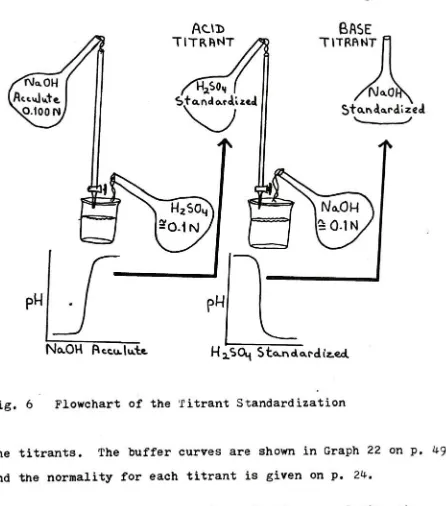
After the titration equipment was _organized, an acid and a base

titrant had to be mixed and standardized. Six liters of each titrant

and one liter of 0.100 N sodium hydroxide Acculute were mixed. The

sodium hydroxide Acculute solution was used to standardize the sul

furic acid titrant

(See

Figure

6).

The standardization was done

by

titrating

the Acculute solution into 10 mis. of the sulfuric acid.

The standardized sulfuric acid titrant was _then used to standardize

the base titrant

by

titrating

the standardize sulfuric acid into

10 mis. of unstandardized sodium hydroxide titrant. The buffer curves

were plotted and the endpoints were used to find the _normality of

2

Acculute is concentrated volume that has been _accurately prepared

18

Flowchart of the Titrant Standardization

AC\3>

TITRMT

Figure 6

BASE

TlTRftMT

Standardized

NaOH RcculUU

HaSO-

Sta.ndardiz.edl

Fig. 6 Flowchart of the Titrant Standardization

the titrants. The buffer curves are shown in Graph 22 on p.

49

and the normality for each titrant is given on p. 24.

b)

Standard _operating procedures for the manual titrations

The standard _operating procedures for the manual titrations

done at the Institute are described below. Concentrated solutions

of the ingredients that make up the known samples are put into the

5

ml. burets. A 250 ml. beaker is filled with

75

1 ml. of distilled [image:24.570.44.490.88.594.2]

19

are added to the beaker to make the equivalent of a 1 ml. sample

of a photographic

processing

solution at a stock

dilution.

If an

unknown solution is

being

titrated,

one milliliter is measured into

the beaker of distilled water.

The pH meter is standardized to the pH 9.00

buffer;

the sample

is placed on the magnetic stirrer; the stirrer is started; the pH

probe is

lowered;

and the titrant buret is filled and centered over

the

beaker.

When the sample's pH is stable to 0.01 pH _units, the

reading is recorded

in

tabular form and on a graph. The graph is

used to determine the volume of titrant to

add, depending

on how

close the pH is to an endpoint. The 50 ml. buret is then used to

deliver the predetermined volume of titrant and the pH is again

allowed to stabilize. This process continues until a preset termina

tion pH has been exceeded. At this

time,

the mixer is turned off;

the pH meter put on standby; the probe is raised and rinsed with

distilled water into the finished sample. The beaker is washed and

a new _{titration may} begin.

IV.

Evaluating

the Buffer Curve Analysis

a)

Monitoring

the _stability of the concentrated sample solutions

The concentrated solutions are stored in

125

ml. erlenmeyer

flasks with rubber stoppers. The initial storage _volume, after

the solutions are _made, is such that _only 2 mm of air space is

allowed between the rubber stopper and the solution, but as the

solution is _used, the volume of air in the flask

increases.

As the

experiments were carried out over a three week _period, samples were

20

air. After three _weeks, all fresh solutions were mixed and titrated

within 24 hours to

further

measure the effects of air and time.

These checks continued for the fresh solutions. The buffer curves

for the fresh and old solutions can be compared in Graph 4 on p. 29.

b)

Factorial Experiments

A number of two level factorial experiments were designed to

include

the combination of ingredients of photographic processing

solutions. The concentrations of the ingredients were set to ex

ceed the typical range of concentrations used in photographic

processing solutions. Thus a typical range of 30 g/1 to 100 g/1 of

sodium sulfite might have a concentration range of 10 g/1 to 100 g/1

in

one of these factorial experiments.

3 A 2^

factorial experiment was performed for the ingredients of

an activator - _sodium

sulfite, sodium

hydroxide,

and Na^EDTA

(See

Graph

5

on p. 30). From these results, a 4 factorial experiment

was designed and carried out _using sodium sulfite and sodium hydroxide

(See

Graph 6 on p. 31). To evaluate the ingredients of a concentrated

u

developer,

a 2 factorial experiment was designed with these in

gredients - _sodium

sulfite,

hydroquinone,

potassium

hydroxide,

boric

acid, and a constant level of ethylene glycol to allow the high

concentration of hydroquinone to go into solution

(See

Graph

7

on

p.

32).

These factorial experiments were performed at Versa Chem

Corporation with the automatic titration system.

With the manual titration _system, two other factorials were

designed. The first factorial included the ingredients found in

21

followed the constiuents of Kodak's D-72 developer. The buffer

curves for these factorial experiments are illustrated

by

Graph

8

on p.

33

and Graph

9

on p.

34,

respectively. Kodak's D-76 developer

contains sodium _sulfite,

hydroquinone,

_elon,

borax,

and potassium

bromide while Kodak's D-72 developer uses sodium carbonate as a

buffer

instead

of

borax.

The

ingredient

concentrations had a range

which is

typically

used for the purpose of a photographic

developer.

c) Single

ingredient

concentration series

Single

ingredient

concentration series were also run for a number

of ingredients found in photographic

developers,

_activators,

fixers,

or stabilizers. These single ingredient titrations included aluminum

sulfate, acetic acid, sodium _sulfite,

hydroquinone,

_elon, potassium

bromide,

boric acid,

borax,

sodium _carbonate, sodium

thiosulfate,

and potassium alum

(See

Graphs 10-20 on pp. 35-47). Samples of D-76

and D-72 were also titrated and illustrated in Graph 21 on p. 4a.

When the single ingredient concentration series for potassium

bromide was _evaluated, it was found that a change in the ingredient's

concentration showed no significant change in the buffer curve with

concentrations four times larger than would be use in photographic

processing solutions. Further tests were carried out to see

if

potassium bromide changed the buffer curve with other ingredients

present. This was done

by titrating

a 10 g/1 solution of potassium

bromide into a solution that contained 1 ml. of D-76

developer

and

75

mis. of distilled water. After 20 mis. of the potassium

bromide

titrant were _added, the _resulting sample was titrated _normally with

22

curve for D-76 developer without

any

extra potassium bromide added.

The results can be compared

by

_referring to Graph

15b

on p. 42.

d)

Further evaluations

After

analyzing

the factorial experiments and single ingredient

concentration _series, those ingredients that could be _{significantly}

detected within the typical concentration of photographic _processing

solutions were chosen from the D-76 and D-72 developers. The exact

concentrations of these significant ingredients were mixed and

titrated to compare their buffer curves with the developer solutions

made from Kodak

(See

Graph 4 on p.

29).

In order to obtain a larger pH _range, samples of sodium sulfite

had 10 ml. of sulfuric acid added to them after which

they

were

titrated with the base titrant. Graph 12b illustrates the buffer

curves with the extended pH. These buffer curves were compared to

titrations without acid _added, to determine if there is a distinct

advantage to an increased pH range.

e) Mathematical representation of data

The relationship of a single ingredient's concentration to

volume of titrant required to reach the final endpoint was plotted.

From the linear plots, the slopes were determined for sodium _sulfite,

sodium _carbonate, and the combination of the two at equal concentra

tions. These experimental slopes were compared to theoretical slopes

calculated from the knowledge of the ingredient's molecular weight

and the titrant's normality. The theoretical and actual calculations

23

Using

the assumption that acid and base titrants dissociated

100$,

their theoretical relationships between pH and volume of

titrant were calculated. The relationships were calculated for

sodium hydroxide titrated with sulfuric acid and sulfuric acid

titrated with sodium

hydroxide.

These relationships are written

out on p.

25.

The plots of these relationships were compared to

the experimental results obtained when the titrants were standard

ized.

This is

illustrated

in Graph 22 on p.

49.

The results from this research are designed to determine the

feasibility

of the analysis. In

doing

_so, the possibilities for

fitting

the buffer curves to a mathematical model were

investigated.

A number of mathematical models were considered

-linear regression

through

transformation,

multicurve _regression, the method of principal

24

RESULTS

Automatic Titrator Pump Accuracy

Primed the _pump once ;

delivery

tip

touching

buret

No _priming;

delivery

tip

touching

_buret

-Two minute time

lag

between tests;

delivery

tip

suspended above buret

-No time

lag;

delivery

tip

suspended

-Delivery

tip

touching

-X sd n

5.033 0.023

3

4.984 0.0434 11

4.947

0.0231

3

4.998 0.0108 6

4.996 0.0440 14

Automatic Titrator Standard Error

Standard Error = _0.04850

n =

8

_{replicates of buffer curves}

Time/titration = _{16 min./35}

ml. of titrant added

(initial

algorithm)

6

_min./35 ml. of titrant added

(final

algorithm)

*

Manual Titration Standard Error

Standard Error = _{O.O636I n} = _{6 replicates of buffer curves}

Time/titration = _{30 min./35 ml. of titrant added}

Standardization Values for the Acid and Base Titrants

Acid Titrant

-0.1005

N sulfuric acid

Base Titrant

-0.0975

N sodium hydroxide

(not

_used)

0.1000 N sodium hydroxide

(Acculute,

used for

titrant)

Theoretical Calculations for Ingredient Concentration vs. Volume of Titrant

Sodium sulfite

(g/1)

=126 g/mole x 1000 samples/liter x 1 _mole/eq x

0.0001 eq/ml x Volume of Titrant

(ml)

=

12.66?

_{x Volume of Titrant}

(ml)

(Assumed

1 _mole/eq because the pH started below the first endpoint)

Sodium carbonate

(g/1)

=

105.99

_{g/mole x 1000 samples/liter x 1 mole/2}

eq x

0.0001 eq/ml x Volume of Titrant

(ml)

2

Actual Calculations for Ingredient Concentration

vs.

Volume of Titrant

Sodium sulfite

(g/1)

=

14.8

_{x Volume}

of Titrant

(ml)

Error = _{Actual slope/Theoretical Slope}

=15%

Sodium carbonate

(g/1)

=

6.061

_{x Volume}

of Titrant

(ml)

Error =

13.8%

Mathematical Model of Buffer Curve

by

Chemical

Theory

Assumption: All ingredients dissociate

100%

Acid Titrant

-pH =

14

+

log

(equivalents of _starting solution - _milliliters

of titrant x 1

liter/

1000 ml x 0.1 _equivalents/

liter)

Base Titrant

-pH =

GRAPH 2

Digital pH Meter Amplifier vs. Time

27

26

GRAPH

3

29

Sodium Sulfite and Sodium Carbonate

i~

C 'm rrt > M

GRAPH

5

O o7

.X'.] SI o in 1.1

iiJJl

3

1_I

r

-1 I4- L*~.

ir

I 4ft

I*"

"ol|jTl-i-l1-L_*_x_t_i_a_i_j.-iiL

uT-r

'~W

<_TJ CT"J

30

odium

Sulfite,

Sodium

Hydroxide,

and _Ethylene Diamine _Tetraceti^c Acid With 4 Moles of Sodium Ion - 2}

31

Sodium Sulfite and Sodium Hydroxide -2

---GRAPH 7

Potassium

Hydroxide,

Hydroquinone,

_Sodium

Sulfite,

and Boric Acid with constant level of ethylene glycol

24

Factorial

Experiment

32

33

GRAPH

8

Hydroquinone,

Elon,

Sodium

Sulfite,

and Borax

2

Factorial

_Experiment

AJA- LLril-L-:"'5 -^i'ULlfiLLLLL^loK:::L.L ::Li. '': -.; |> .

i*i Hjiain--;*- _LaoaiOouTT

-MtfiL^fcWj-.

1 --IO

_*=^AS

. ..l

-aa

r,: at.11 al

l _:o o O _ !? 2ft 3

0;--- _ _

-jOo _^

GRAPH

9

V

i

! "5

34

10

I J

-! oi

c -.01

X

sft

t

4J

-3 _S.5

>/\

<-j f -i t

-i.iM

c-a o 31_2

rfl^lJt ill 1' ₁ rt

j

ri '~tt /

/

n

/T-r|

J o

Hydroquinone,

Elon,

Sodium

Sulfite,

and _{Sodium Carbonate -J}

4

Jr.APK 10

Aluminum

Sulfate

-Single

Ingredient

Concentration

Series Buffer Curves

c

il&h-1V.OO-

-10.00

.-I.. CU^t^i

. . ;

z _>

-"'---;-: :y~

"

:

,-,-lL, ...j.,.-H

,-; '-: ' : :..\'

i

JJ~A~~~r~~~''

--j-j--rj]-y:y. ;-a|-aa:7

GRAPH 11

Acetic Acid

-Single Ingredient

Concentration

Series Buffer Curves

36

(

.aZ

::-: 20m

i/i

^A0n\

_{$jojLaSyyyy\ ]Z}::.['.... _:-( . 1mt fL20\/it

Wf/\:y

LL

>'"

-- ...:.a-'_-./

^ ₃ 2i*\\ _o*\ Ibrnyg

IA

*ws-4JLLL

!/

:

j

LLL/ ._. ._ -r:r?L -'At

m&

Mfa.

L,i-:::-f7i-:! r.rz.:. a^LTaLLLJ \V.Wr

... . AAA L~L:JL L--:L , ':

t:'A:~:'r

;:;;.;

.M:i---i::i

Ml]

rrr .

~y.j "--l':': i

J:L";

.. .: ':'

J

:

-j . !

[

J -: 1 4

-Lll

[a f:~:

: : jj : jj. .... :

...;:. :-::L-..:

LRLLLi AA: :

'AJr

JM|L:

;

L ;.:::: LL

jLLL' \ 1

-1*00 "

'-.'I-L-LL

:!!:f ';l:_llJl-ll:l- J.rJ.r. : _zyyy .::-!:- !. -i:. .4. :: !

:;'i:;j

r^ LL:--fL/.; -:| A-JA '.',.*' rrrrJArA -A:~. -M .v>

ZAriAAAirA'^

J\

Ajy-Z-: .:!:.:.;:

!

: .Va Aft - --r-r-jy-^.J-A^r lAAAlA 1 ' -I."."! LiLJa.; 7J-HLL--;-yz ::rr?' !:--.-:-..

JJJJAr._ .: - :.-..j.:.r-- :::.!

:-}?LLL

:-::":ir :L . La i

..j

AA. L :LL!L:.L. : ,. .: : 1

'

:t. ' '

!. ..jj.

l-ll-l-K-lll;-::

-- -!--

:--T f\r\ ''l-lI-tl

iii :_~J-A:

. Ar "-"

: ! Jr.. :LL;L-i

' /.OO yZrZZ ""L-L :i:L;fe-a ... "LLL-rLr A ''

'.

\

L-'LLaJLLiziaa :

... ...--':. ...

pH

LLtL-iLji-:

rr JJjrrlAJ'A ..

L-^iii -yj ;.. : : ;: ; .. Z.AA:

. 'j:::P:J.hAJ:r ^. .

LLL;. r:r: L r: :

: _f ::...:-: ;

7

y..:\.:m.-.j.r

-".- -; _L -";:. " (p.00" ...yM

m:/f-yT

J-:].

]

_A\ Arr

..._..:. -L:--:~ .--": J.-.:... -..:-.

Zy

' -r\J. .". :.L-:

AAy'j

.-.. ;

/;....

rj/r >:'-. :"!:'/:-'

/

O.w

''m//^i

i

l - -" : "

LLL .. .

/

yy

LLL-.L-vL

\y

r:

T.VR--'1/

\r . !. : ;

.. _, .. . ...j._.. ^ .._.... :.;

-;:... . ...y..

L:L..;

:-L.i

3.oo-2.oo

4

r.

- _h- ₍ 1 _-j

-

-t _^ ~_{l ]}

i-

₁

X .3 to %

to _M .^ 13ml

T7

GRAPH 12a

Sodium Sulfite

-Single Ingredient

Concentration

Series Buffer Curves

-U.00-1- voo a/i. r)Z

.-..,. . I.

i'-]_ I

3u_!L_50Vl..LLy_Ul

yxm^o?: . ML___:i___J__.

VoWt

o^ ^Vraot

^

0.\oo5N)

Hz^Oi-GRAPH

12b

Sodium

Sulfite

with base titrant

-ingle

Ingredient

Concentration

_{Series Buffer Curves}

(extended

pH _range)

?jOL|i^&_7lLOUUi.aLL/4o ml

":'hMMM1le;

21) Squaresto theliu:h

Volant

39

GRAPH

13

Hydroquinone

-Single Ingredient

Concentration

Series Buffer Curves

feo--

wo-T\

~cfc

\0$

/j

_{o"SoJi*LS^i*-te}

-Iwtv\ OrX \

OO3

/| Of Spdl.u.- ,uJfi* Iw\\ o? 100-^fi or -s>ea.u,RN ->Uk.\itac

\tr\

Q.

_fi?

/

V c

H^<A.co<^aao<\^

^

-1N1

-c ,1A'- --/---_;

-^1,7-,L-M-J-L^-iidf-SoJUtun3^l?<

--:

20 Squarescnitn-In. h

\JoVuLNe

_o^c

T'Ara^^

"0.I0C6N H2.S04

GRAPH 14

Elon

-Single

Ingredient Concentration

_{Series Buffer Curves}

kQ

HKOr .i^_d_!a_jjtv\ o .10LT

/

lr c

El

OfO '->".- <- -

rt---*jLL: .ii Li L: . / todliur,

Su.Wrf_;

pH

/.o v.O 3.0 M.O &'0 7'0 ^ '.--0 "* '3- mi

''' _{; ! i}

'

:

GRAPH 15a

Potassium

Bromide

-Single Ingredient

Concentration

Series Buffer Curves

4l

rtf-oe-l:.

-ti*eW-

tGteO?-BBMl^t^ ^^4

S*^

e*rW

x

Ml! Mo*

jftS

*f-; -te

iEa

HL]S

*fcoer

pH

7=nsn-M*

i._*._

!--t-rr-hrrr ^t~ vvfrv U-r-.frr:r-r rl-y 1LLL iJLLLL: T~r .,....>: :v.-;.t.j.: j. ..-:.-:(: -\rr. -r^rrt--?:v..p: TilLn^ u_:|. .-:l "I --j-

:.-:,-

i-i-:l::

V

.-I 3coo

2^w>i t * 4- + 4*- _{H 1}

1-20Viuar.-* IniP,In. fi O 1 Z i M 5 <e T ^ 1 10 a U

W ₁₅ id ^ il n ici w is _^35

GRAPH x5b

D-76 with and without _{Potassium Bromide Added}

42

a,

iw-\

^

_..3-7

v

lK^\WTU)*jf_i

felt .-* to m .. ...3

Volume

0^ TiicoLftV

(rr\\^

O.lOOSlO

H^O-GRAP.n lb

, _ Boric Acid

-oingle

Ingredient

Concentration

Series Buffer Curves

4^

;-H-oo--tooo

$.&--_-L. .-x*.

iO^c/i

ot

l&oric

AciA

">

Constat

Ul\

f-~

7.|

(-..

:: . I ^7

-5rO--rL-iLL!:, -:

i

-.

-:--jr--3.00

y-y-200 -i 1- -1 h

(!o

~i!o

yo~<.- sio fc.0 7-0 3.0 9,0

fao 110 U/> ti.o.

44

GRAPH

17

Borax and Sodium Carbonate

-ingle Ingredient

Concentration

Series Buffer Curves for each

GRAPH 18

r

Sodium

Carbonate

-Single Ingredient

Concentration

Series Buffer Curves

45

, ;....

yj-.jy

1.

t-L^

\-r~-\~

j;-:

\

_:

2-00 H 1- _{A 1} 1 1 \

M.o t--0 S.O loo \X.O m)

GRAPH 19

Sodium Thiosulfate

-Single Ingredient Concentration Series Buffer Curves

46

-~

c

-U.to-- -4~ lreJl

4

2Wv*/A L._...L L.J...L

'

(<JI -S XtoO^/l C ^v fiili^nJatlki. C0BJAj3j\AJjyOiv

'^)

J.O *,0 '.O v,o 5.O 6.0 7.0 S.o 9,0 .OiO U.Q

GRAPH 20

Potassium Alum

-Single Ingredient

Concentration

Series Buffer Curves

4?

^

*

I

nM of

30^/

1

^

' A. m\ of _\5ajr/|

MiOo

3,oo

---I 1- H

\-2- 3. H t . 7 8 ID Ij. '3

48

GRAPH 21

Kodak"

s D-76 and D-72

Buffer Curves

X

-'

o-Sn-\ O^ -~?Vi

-[hOfrf3,- '- O.Errv\ O^

l>-7^

GRAPH 22

.trant

Standardization

Buffer Curves

49

U.00

U.06

\6n\l ia-.o'tt

ExPfcRTnfcNTfVu

c

5

T.HORll\c,M.c

*.oo

__4

QOO

i_.:"l;]WM.nA*L^i*ftt.

: _

> (,(40H uaKmuik tOmlittr^

rn9kfWeei\a.JtJtjA yttAiclrfK eS H*^>0i- -WVrft-Viorv

SI

..5

j

;~

M ;^^yN^ 0*000

lagg&fltej

5C

GRAPH

23

Ingredient Concentration vs. Volume of Titrant

for the Final Endpoint

_o

5-DISCUSSION

I.

Automatic

Titrator

a) Improvements to the system

Initially

the automatic titrator took on the average of 16

minutes to titrate a sample

by

_adding

35

ml. of titrant in 1 ml

increments.

However,

the main advantage of the automatic titrator

is to be able to submit a number of samples for titration at once.

At this speeti the sixteenth sample would be titrated four hours

after the first

titration,

provided all of the samples required

an average of

35

additions of titrant. In this time _period, samples

can reacte with the air. This can be seen in Graph

6

on p. 31.

The curve number represents the order of the samples on the titrator.

The graph shows a large _variability between buffer curve 1 and

15.

The last samples to be titrated show a buffer curve shifted to the

left more than would be expected. Also when the experiments used

hydroquinone with low concentrations of _{preservative,} aerial

oxidation was noticed before these samples were titrated.

Thus,

to decrease the error, the time per titration had to be decreased.

The algorithm was changed in _many ways to increase the speed

of the automatic titrator. The sum of these changes decreased the

time per titration from 16 minutes to

6

minutes for the addition of

35

mis. of titrant. The speed increased

by

a factor of

2.5.

Thus

the sixteenth sample would be titrated _only

li

hours after the

first titration, if all samples required

35

mis. of titrant. How

ever runs do not require such large volumes of titrant to be added

52

unstable samples could be titrated first or smaller runs could be

used.

b)

Testing

the automatic titrator'

s environment and equipment

Since the pH is

dependent

on

temperature,

tests were run to

monitor the temperature in the automatic titrator 's environment

(See

Graph 1 on p. 26). Over a 24 hour period there are three major

factors that determine the temperature of the titrator samples.

The

building

is an aluminum structure which absorbs the sun's

radiation effectively. When the sun rises the

laboratory

tempera

ture rises

4.5C.

Likewise when the

building

goes into shadow, the

temperature _{significantly}

decreases.

The second factor that affects the temperature of the

laboratory,

is whether the door from the

laboratory

to the plant is opened or

not. The

laboratory

is not heated so it must absorb heat from the

floor and walls when the

laboratory

door is closed. With the door

opened, the

laboratory

temperature is affected

by

the thermostat

in the plant.

The third factor is the mixer motor. The temperature of the

mixer motor increases the solution's temperature

by

0.7

C over a

six minute period of time.

The temperature should remain _relatively constant

during

a run

of a number of titrations to decrease the affect of temperature on

high and low pH readings. It was found that the temperature is

stable to kC between 12i00 and

18:00.

The average temperature

between these times is

22.0C.

With the

laboratory

door opened and

53

These are the optimum times when the titrations should be run for .

a minimum of pH error.

The pH meter amplifier was also monitored for a 24 hour period

(See

Graph 2 on p.

2?).

The amplifier drift correlated

87#

with

the temperature of the

laboratory.

Thus,

there is no major problem

with amplifier drift outside of the temperature's influence.

After

the titrant _{pump had} been calibrated to a

5

ml. buret for

a _week, the _pump

accuracy

and precision was tested under a number

of conditions. The results have been tabulated on p. 24. When

the titrant

delivery

tip

is

touching

the _measuring

buret,

there is

capillary action to draw some of the solution out of the tip. The

result was an 0.0331

increase

in the standard deviation. With time

the _gravity pulls some of the solution down the hose and back into

the titrant _pump to decrease the volume delivered, when the _pump

is primed once before each

test,

there is an

0.049

ml. increase

in the volume and an 0.0204 decrease in standard deviation. When

a time

lag

is imposed between

tests,

there is more of a chance for

the solution to drain into the titrant reservoir. In comparison

to the tests with the pump primed, there was an 0r086 ml. decrease

in the average volume measured when a time _lag was

imposed.

To

help

eliminate the gravitational _effects, the titrant _pump, titrant

reservoir and

delivery tip

were put at the same height. With the

delivery

tip

suspended and the components at the same

height,

the

best accuracy and precision were attained - _average =

4.998

_and

standard deviation = 0.01084 for sample size of

6.

The accuracy and the precision of the titrant _pump is more

54

while the buret measurements can correct the error on the next

addition of titrant. If the

buret

measurement is over or under

the desired _volume, the next addition of titrant can still deliver

a correct total volume

desired.

_{If the titrant pump's} average volume delivered is"

too

larger

or too small than the error will

accumulate as each offset volume is

delivered.

However,

with the titrant _pump components at the same height and the

delivery

tip

suspended, there will be a

99. 7#

chance that the volume of titrant

delivered will be 34.986

+O.O33

mis. for an expected value of 35.000 mis.

To determine the effects of the initial volume of water on the

buffer curves, this volume of water was varied. A 20 ml. increase

in

volume decreases the

starting

pH

by

about

0.05.

The largest difference in pH due to a 20 ml. difference in the initial volume

of water was 0.40 pH units at the activator's first endpoint

(See

Graph

3

on p. 28). If the initial volume is held to

75

+2 _ml., the pH should remain within 0.04 pH units.

c) Standard error of the automatic titrator vs. the manual titration

The automatic titrator' s repeatability has proven to be better than the manual titrations. The automatic titrator's standard

error was 0.0151 standard deviation units lower than the manual titrations. The response variable is pH. The resolution of the

automatic titrator system depends on the ingredient because different

ingredients are more sensitive to additions of an acid or a

base.

For sodium sulfite with a sample size of

3.

there is a

95%

chance

55

carbonate, there is a 95< _{chance of}

detecting

_{a concentration of}

1.8 g/1 or

larger

when a sample size of

3

is used.

II.

Evaluating

the Buffer Curve Analysis

a)

Monitoring

the

stability

concentrated sample solutions

The tests were performed to resolve _any change in the buffer

curve _{characteristics of an}

ingredient

_{due to the concentrated}

solutions'

long

periods of storage. Over a three -week period when

the solutions were _used, the volume of air in the storage flasks

increased,

but the effects to the buffer curves were

insignificant.

The buffer curves labeled B and D

in

Graph 4 on p.

29,

do not show

a significant difference between the fresh and old solutions. These

results were based on the concentrated solutions of sodium sulfite

and sodium carbonate.

b)

Limitations in the buffer curve analysis

The buffer curve analysis is subject to a few

limitations.

One

limitation that applies to all ingredients can be expressed

by

the

saying,

"only

the _strong survive."

Only

those ingredients with

concentrations that are close to the ingredient with the largest

concentration _may be

detectable.

In _general, ingredients with con

centrations greater than 1/1Oth of the

largest"

concentration is

detectable.

This can be seen in the graphs of the factorial experi

ments

(See

Graphs

8

and

9

on pp.

33

and 34). The equivalents of

titrant required to neutralize the largest concentration will

determine the resolution of that analysis. If there is an ingredient

c.

J-volume of titrant would have to increase

by

a factor of 10 to get

the same resolution as the

largest

ingredient.

This is impractical

for a

titration

_using 30 mis. to form the buffer curve, because the

volume of titrant would have to

increase

to 300 mis. The automatic

titrator would tak# 1

hour

to titrate the sample and the manual

titration would take

4 hours.

A second

important

limitation

of the buffer curve analysis is

that some ingredients are not suited for this analysis. The con

centrations

typically

used in photographic _processing solutions are

not detectable when an 0.1 N titrant is used. Some ingredients

may not affect the pH at all. Such ingredients include potassium

bromide,

hydroquinone

(See

Graph

13

on p.

39),

boric acid

(See

Graph 16 on p.

43),

and Na^EDTA (See Graph

5

on p. 30). Borax and

elon are

barely

detectable at the concentrations

typically

used in

photographic processing solutions

(See

Graph 17 on p. 44 and Graph

14 on p.

40,

respectively). In the case of sodium

thiosulfate,

the

ingredient doesn't resist the addition of an acid. Instead it

converts into another compound without _resisting the additions of

titrant. With potassium _alum, the rate of the reaction to reach

equilibrium is slow. When the titrant is

added,

the pH changes

quickly

to put the chemical reaction in the forward

direction,

but

it passes its equilibrium and _slowly reactes in the reverse direction

to reach its equilibrium. The rate of the reaction is slow in the

reverse direction.

Thus,

the pH will not stabilize for a number of

minutes after 1 ml. of titrant has been added. Such a titration

may take an hour or so to do with a manual titration. Phis slow rate

of reaction makes the buffer curve analysis undesirable _for use with

57

The analysis has been able to resolve a number of ingredients

used in photographic

processing

_{solutions. These}

ingredients

include

sodium

sulfite,

sodium _carbonate, acetic acid, aluminum sulfate,

sodium

hydroxide,

and potassium alum. These ingredients can be

found in photographic

developers,

fixers,

_activators, or stabilizers.

There was no

detectable

change in the buffer curve with potassium

bromide alone in a solution at concentrations much larger than is

typically

used in

processing

solutions

(See

Graph l}a on p. 41

)

.

It was also shown that these concentrations had an insignificant

influence on the buffer curve when other ingredients were present.

The five ingredients in D-76 were subjected to 20 mis. of a 10 g/1

solution of potassium bromide without _changing the pH

by

more than

0.02 after the first milliliter was added. The buffer curve for this

solution showed a small change when compared to an unaltered sample

of D-76. The small change was the result of an increase in potassium

bromide concentration that is 40 times the concentrations _normally

used in photographic _processing solutions.

4

From the 2 factorial experiment with the ingredients used in

D-72

(See

Graph

9

on p.

34),

it was determined that _only sodium sul

fite and sodium carbonate were significant ingredients. These

ingredients*

concentrations _{significantly} affect the buffer curve.

A buffer curve was performed with these two significant ingredients

at the concentrations used in Kodak's D-72. This buffer curve was

compared with the buffer curve for the solution of

D-72,

which was one

of Kodak's products

(See

Graph 4 on p. 29). The significant dif

ference between buffer curves E and F _may be explained

by

the _grade,

58

can be _up to

6

g/1 of sodium carbonate or 12 g/1 of sodium sulfite.

This analysis has been

designed

to determine the constiuents of

unknown solutions with

any

_{grade, age,} or assay.

However,

it is not

the purpose of this analysis to find the constiuent's concentration

for the specific grade that the unknown solution's manufacturer uses.

An equivalent solution is required to match its performance and not

necessarily the exact concentrations and grades.

Thus,

this difference

in

ingredients

is

insignificant

if

the equivalent buffer curve gives

equivalent performance in the field tests.

c) Further evaluations

The

increasing

of the pH range to include the pH above and

below the sample's normal pH .has a limitation with the titrants

being

used. If a specific volume of an acid titrant is added to a

sample, the base titration will not return to the same _starting pH

in the same number of equivalents

(See

Graph 12b on p. 38). This

will be discussed further below.

However,

if the shape is desired

from the extended pH range, this method is an aid. The extended pH

can show the number of endpoints to

help

identify

ingredients _easier,

but it is not an accurate measure of the ingredients* concentrations.

d)

Mathematical representation of the data

The single ingredient buffer curves demonstrated

linearity

between the concentration of the ingredient and the volume of titrant

required to reach the final endpoint. Phis was shown for sodium

sulfite and sodium carbonate

(See

Graph 12a on p. 3'7). This graph

59

(Curve 2)

to 100 g/l

(Curve

3)

_{will double the volume of titrant}

required to reach the final endpoint. This _relationship is shown

in Graph

23

on p.

50,

However,

when the theoretical _relationship

between a single

ingredient's

_{concentration and the volume of titrant}

required to reach the final endpoint was

determined,

there was as

much as a

15#

difference

_{from the experimental relationship. In}

the case of sodium _sulfite, the error could be from the _starting pH.

The

starting

pH of the single ingredient of sodium sulfite has

already

past its first endpoint. Thus one of the two species in

sodium sulfite has been neutralized. The degree of neutralization

is not

known,

but it is suspected that it is not

fully

neutralized

because the theoretical _relationship for sodium sulfite based on

one equivalent per mole is too small and the _relationship based on

two equivalents per mole is too large as is shown on p. 24 in the

Results section. Some other error _may be introduced

by

the grade,

age, and _assay of the

ingredients.

This could explain the error

found with sodium carbonate.

The _relationship between the concentrations for more than one

ingredient and the volume of titrant required to reach the final

endpoint is not the sum of the individual ingredients

(See

Graph 4

on p. 29). The sum of the volumes of titrant required to reach the

final endpoint for sodium sulfite

(Curve

B)

and sodium carbonate

(Curve D)

is _{significantly} larger than the volume of titrant for

the buffer curve

(Curve

4)

whose solution contains the two <