in the central molecular zone
.
White Rose Research Online URL for this paper:
http://eprints.whiterose.ac.uk/91178/
Version: Accepted Version
Article:
Koepferl, CM, Robitaille, TP, Morales, EFE et al. (1 more author) (2015) Main-sequence
stars masquerading as Young Stellar Objects in the central molecular zone. Astrophysical
Journal, 799 (1). 53. ISSN 0004-637X
https://doi.org/10.1088/0004-637X/799/1/53
[email protected] https://eprints.whiterose.ac.uk/ Reuse
Unless indicated otherwise, fulltext items are protected by copyright with all rights reserved. The copyright exception in section 29 of the Copyright, Designs and Patents Act 1988 allows the making of a single copy solely for the purpose of non-commercial research or private study within the limits of fair dealing. The publisher or other rights-holder may allow further reproduction and re-use of this version - refer to the White Rose Research Online record for this item. Where records identify the publisher as the copyright holder, users can verify any specific terms of use on the publisher’s website.
Takedown
If you consider content in White Rose Research Online to be in breach of UK law, please notify us by
Preprint typeset using LATEX style emulateapj v. 04/17/13
MAIN-SEQUENCE STARS MASQUERADING AS YOUNG STELLAR OBJECTS IN THE CENTRAL MOLECULAR ZONE
Christine M. Koepferl, Thomas P. Robitaille, Esteban F. E. Morales, Katharine G. Johnston
Max Planck Institute for Astronomy, K¨onigstuhl 17, 69117 Heidelberg, Germany
Received 2014 July 13; accepted 2014 November 13
ABSTRACT
In contrast to most other galaxies, star-formation rates in the Milky Way can be estimated directly from Young Stellar Objects (YSOs). In the Central Molecular Zone (CMZ) the star-formation rate calculated from the number of YSOs with 24µm emission is up to order of magnitude higher than the value estimated from methods based on diffuse emission (such as free-free emission). Whether this effect is real or whether it indicates problems with either or both star formation rate measures is not currently known. In this paper, we investigate whether estimates based on YSOs could be heavily contaminated by more evolved objects such as main-sequence stars. We present radiative transfer models of YSOs and of main-sequence stars in a constant ambient medium which show that the main-sequence objects can indeed mimic YSOs at 24µm. However, we show that in some cases the main-sequence models can be marginally resolved at 24µm, whereas the YSO models are always unresolved. Based on the fraction of resolved MIPS 24µm sources in the sample of YSOs previously used to compute the star formation rate, we estimate the fraction of misclassified “YSOs” to be at least 63 %, which suggests that the star-formation rate previously determined from YSOs is likely to be at least a factor of three too high.
1. INTRODUCTION
Various indirect techniques based on diffuse emission are traditionally applied in order to measure the star formation rate (SFR) of galaxies throughout the Uni-verse. These common techniques use star-formation trac-ers such as free-free cm continuum, Hα, and far infrared emission to indirectly infer the rate of forming stars (for details see review by Calzetti 2013). Free-free emission (or Bremsstrahlung) emitted from ionized electrons, and recombination lines of ionized hydrogen (e. g. Balmer se-ries Hα) both trace gas ionized by young massive stars. Another method is to use the infrared flux as a tracer, since the UV radiation from young massive stars is also absorbed by surrounding dust and re-emitted in the in-frared. Combinations of various diffuse tracers (such as 24µm emission together with Hα) are now commonly used. All these conventional methods usually agree but trace only the high-mass star formation rate, and require an extrapolation to lower mass stars.
For the Milky-Way, we have the opportunity to di-rectly estimate the SFR by counting individual young or forming stars, which if calibrated with caution is a pre-ferred method as it accounts for the actual sites of star-formation. With theSpitzer mid-infrared survey ”cores-to-disks” (c2d, Evans et al. 2009) the SFR of nearby star-forming regions was estimated to be 6.5×10⁻⁶ to 9.6×10⁻⁵M
⊙yr−1by counting YSOs (down to low mass objects), assuming an average mass of 0.5 M⊙and a star-formation duration of 2 Myr. For the first timeRobitaille & Whitney(2010) calculated the total SFR of Milky Way Galaxy by counting sources showing a mid-infrared ex-cess at IRAC wavelengths, using a population synthe-sis model to extrapolate the number of sources beyond the detection limit. They found an overall SFR for the Milky Way of 0.68 to 1.45 M⊙yr−1. This is in agreement
with techniques based on diffuse emission tracers: in-deed,Chomiuk & Povich(2011) demonstrated that once the SFRs derived from the different methods are nor-malized to the same assumptions (for example for the IMF), the methods are all consistent with a value of 1.9±0.4 M⊙yr−1.
Yusef-Zadeh et al. (2009) calculated the SFR of the Central Molecular Zone (CMZ) directly from their 599 classified YSOs with 24µm emission and found a rate of 0.14 M⊙yr−1. In order to derive this SFR, they deter-mined stellar masses for each YSO, constructed a mass function, and fit a Kroupa Initial Mass function (IMF, Kroupa 2001) to the peak of the derived mass distribu-tion in order to extrapolate the stellar mass below their sensitivity limit, then assumed the upper limit to the age of 1 Myr for 213 of these objects. When comparing their derived SFR with values from indirect methods (e. g. free-free emission) large differences arise, up to a factor of 10, in contrast with the good agreement seen on the scale of the Milky-Way as a whole. For example, Longmore et al.(2013) found, from their measurements of the total ionizing flux using the free-free emission, that the over-all SFR of the CMZ is roughly 0.012-0.018 M⊙yr−1 for |b| ≤ 0.5◦ and 0.06 M
⊙yr−1 for |b| ≤ 1◦, also covering areas outside the CMZ.
Whether the differences are real or due to issues with either the YSO-counting or the diffuse emission methods has not been established. The estimates based on YSOs could be heavily contaminated by reddened objects older than 1 Myr. In addition to these observational effects, the cm continuum and YSO counting methods may trace different time-scales and thus would be expected to dis-agree, if the star-formation was episodic. In this paper, we aim to determine how much observational effects are able to contribute to this difference.
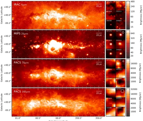
Ro-Fig. 1.—IRAC 8µm, MIPS 24µm, PACS 70µm and PACS 160µm observations of the Central Molecular Zone (CMZ) on a arcsinh
scale. The active star-forming region Sgr B2 (ℓ≃0.5◦,b≃ −0.05◦) and Sgr C (ℓ≃359.4◦,b≃ −0.1◦) are very bright in MIPS 24µm and
PACS 70µm. The objects in the panels to the right show 30 x 30′′zoom-ins of the objects classified as YSOs byYusef-Zadeh et al.(2009),
which have no strong counterparts in PACS 70µm. The numbers refer to the IDs given byYusef-Zadeh et al.(2009). The color maps of
the smaller panels on the right are, in contrast to the main panels, linear and normalized to each panel’s individual extrema. The PSF FWHMs are shown in the top right zoom panel for each wavelength.
bitaille et al.(2006). With this formalism, true YSOs can be separated from more evolved objects. In this formal-ism,Stage 0/1YSOs are very young and envelope dom-inated, with ˙Mgas/M⋆ >10−6yr−1. Assuming that the envelope infall rate goes down in time, this corresponds to an upper limit of the timescale of 1 Myr. Hence, since Yusef-Zadeh et al.(2009) assumed that their YSOs were less than 1 Myr old, these would be classified as Stage 0/1. In contrast, we group more evolved YSOs and main-sequence stars into the Stage 2+ category, with
˙
Mgas/M⋆<10−6yr−1.
In Figure 1, we show the CMZ as observed by the
Spitzer Space Telescope and theHerschel Space
Obser-vatory: the top panel shows the 8µm image observed
withSpitzer’s IRAC camera as a part of the GLIMPSE
survey (Benjamin et al. 2003;Churchwell et al. 2009); be-low is the Spitzer MIPSGAL survey (Carey et al. 2009) using the 24µm band of the MIPS detector; the two lower
panels are far-infrared Herschelimages (70 and 160µm) from the Hi-GAL survey (Molinari et al. 2010) observed with the PACS detector. The Spitzer Space Telescope infrared detectors IRAC (3.6, 4.5, 5.8 and 8.0µm) and MIPS (24, 70 and 160µm) have a Point-Spread-Function (PSF) with full-width 1.66, 1.72, 1.88, 1.98′′ and 6, 18, 40′′, respectively. By comparison, Herschel’s PACS de-tecter at 70, 100 and 160µm has a PSF with full-width of about 4.4, 6.1 and 9.9′′. Hereafter, we will refer to the four bands shown in Figure 1 as IRAC 8µm, MIPS 24µm, PACS 70µm and PACS 160µm, respectively.
[image:3.612.54.544.61.478.2]active star-forming region (e. g. Sgr B2 at ℓ≃0.5◦) the star formation region as a whole is clearly seen in PACS. Obscured main-sequence stars can mimic YSOs, since the surrounding ambient dust is remitting the stellar flux in the infrared (e.g. Whitney et al. 2013). Therefore, in this paper we set out to explore whether objects not seen at wavelength longer than 24µm may not be as young as 1 Myr (as assumed byYusef-Zadeh et al. 2009), and hence may not be members of the Stage 0/1 classification. However, we find instead that although non-detection at PACS wavelengths does not indicate whether a source is a YSO or not, its size at 24µm can be an age indicator. To determine these results, we set up radiative trans-fer models and computed realistic synthetic observations of YSOs (Stage 0/1) and more evolved objects (Stage 2+) in different dust and density environments (Sec-tion 2). To determine, whether more evolved objects (Stage 2+) could mimic YSOs (Stage 0/1), we com-pare the realistic synthetic observations directly with the observations and develop selection criteria that can help reduce contamination from evolved objects such as main-sequence stars (Section 3). In Section 4 we discuss the effects of masquerading main-sequence stars on the SFR of the CMZ. A summary and outlook is given in Sec-tion5.
2. MODELS
To investigate whether main-sequence stars (Stage 2+) embedded in an ambient density medium could mimic deeply embedded YSOs (Stage 0/1) and match the measured brightness profile of the real observation in MIPS 24µm, we performed radiative transfer calcu-lations. We set up 660 models for different spectral types and evolutionary stages in an ambient medium with different dust and density properties. We used the 3-d Monte Carlo radiative transfer codeHyperion( Ro-bitaille 2011) to compute the temperature distribution and create synthetic images. By further modeling the effects of convolution with arbitrary PSFs, transmission curves, finite pixel resolution, noise and reddening, our radiative transfer models are then directly comparable to real observations. Our synthetic pipelineThe Flux-Compensator will be made publicly available in the future1.
2.1. Spectral types & stages of evolution in an ambient
density environment
We modeled main sequence and young embedded O, B and A stars, with temperatures ranging from 44,500 to 8200 K, using in both cases the stellar atmosphere mod-els ofCastelli & Kurucz (2004) as the central stars. We modeled the circumstellar density structure of the YSO models using a rotationally flattened envelope profile ( Ul-rich 1976), with gas infall rates from 3×10⁻⁴M
⊙yr−1 to 3×10⁻⁸M
⊙yr−1determined from the scaling of the envelope density, an outer radius 1.5 pc, and a centrifu-gal radius at 100 AU. We assumed a gas-to-dust ratio of 100. The sublimation temperature, above which dust is removed, was set to 1600 K. For all spectral types, we calculated 10 YSOs models and one additional model
1 For more information aboutHyperion, and to sign up to be
notified once the The FluxCompensatorpackage used here is
[image:4.612.316.564.100.206.2]available, visithttp://www.hyperion-rt.org.
TABLE 1
Stellar data used in radiative transfer setup.
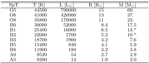
SpT T [K] L [L⊙] R [R⊙] M [M⊙]
O5 44500 790000 15 60.
O6 41000 420000 13 37.
O8 35800 170000 11 23.
B0 30000 52000 8.4 17.5
B1 25400 16000 6.5 13.a
B2 22000 5700 5.2 10.a
B3 18700 1900 4.2 7.6
B5 15400 830 4.1 5.9
B8 11900 180 3.2 3.8
A0 9520 54 2.7 2.9
A5 8200 14 1.9 2.0
avalues from interpolation of the stellar data
without an envelope (but with the constant density am-bient medium), representing a main-sequence object in our simple approach. We use infall rate and stellar mass to classify every model asStage 0/1orStage 2+using the Robitaille et al. (2006) formalism described in Sec-tion1. The stellar data listed in Table1from Appendix E of Carroll & Ostlie(1996) was used to determine the stellar radii and luminosities.
We placed all models within a surrounding ambient medium with a constant density ρ0. We used three dif-ferent ambient density environments ρ0 = [1, 3, 10]× 10−21g cm−3, which are roughly within the number den-sity range of [103; 104] cm−3found for the CMZ (see Moli-nari et al. 2011,Longmore et al. 2013). For the ambient medium, we also assumed a gas to dust ratio of 100.
2.2. Dust properties
For every combination of parameters, described in Sec-tion 2.1, we run the model for two different sets of dust properties. The first was the Milky-Way dust from Draine (2003) with RV = 5.5 and bc = 30 ppm, where RV is the ratio of the visual extinction to reddening mag-nitude, and bc is the concentration of carbon atoms in the medium. Weingartner & Draine (2001) andDraine (2003) favour this combination for the Milky Way and point out that it best reproduces the conditions in the galactic center observed by Lutz et al. (1996). In the second configuration, in order to test the effect of poly-aromatic hydrocarbons (PAH), we additionally used the dust properties byDraine & Li(2007) and as used in Ro-bitaille et al.(2012) with a mixture of 5.9 % ultra-small grains, 13.5 % very small grains and 80.6 % big grains with RV = 3.1 and bc= 52 ppm.
2.3. Realistic synthetic observations
The synthetic images and spectral energy distribu-tions (SEDs) computed by Hyperion are not directly comparable with photometric observations. In order to make these radiative transfer “observations” as realis-tic as possible, we developed a syntherealis-tic observations pipeline called The FluxCompensator. In what fol-lows we will describe it briefly.
TABLE 2
Information about telescopes and detectors.
name zero-point filter pixel size PSF
[Jy] [arcsec]
UKIDSS K 631.e Hewett et al.(2006) 0.4a Gaussian
IRAC 8µm 64.9b Quijada et al.(2004) 1.2b Aniano et al.(2011)h
MIPS 24µm 7.17c MIPS Handbookc 2.4c Empirical
PACS 70µm 0.78f Herschel Science Centerg 3.2d Aniano et al.(2011)h
aUKIDSS Handbook: http://ukidss.org/technical/technical.html
bIRAC Handbook: http://irsa.ipac.caltech.edu/data/SPITZER/docs/irac
cMIPS Handbook: http://irsa.ipac.caltech.edu/data/SPITZER/docs/mips/
dPACS Handbook: http://herschel.esac.esa.int/Docs/PACS/html/pacs_om.html
eHewett et al.(2006)
fhttp://svo2.cab.inta-csic.es/theory/fps/index.php?mode=browse&gname=Herschel ghttps://nhscsci.ipac.caltech.edu/sc/index.php/Pacs/FilterCurves
hhttp://www.astro.princeton.edu/~ganiano/Kernels.html
is provided in Table2, and in the UKIDSS, Spitzer and
Herschel documentation. We convolved the synthetic
images fromHyperionwith the respective PSF after ad-justing the pixel resolution. The original PSF files from Aniano et al.(2011) were used, except the MIPS 24µm PSF, which was directly derived from the observations.
We applied a filter convolution with the corresponding transmission functions from the detectors, and we ac-counted for reddening using the extinction law provided by Kim et al. (1994) and an optical extinction value of AV = 20 mag. Estimates for the visual extinction to-wards the central molecular zone typically range from 20 to 30 mag (seeGeballe et al. 2011), although the higher values likely include a contribution from extinction local to Sgr A; therefore, we assumed a value of 20 mag. Sim-ilarly to Longmore et al.(2013) and Yusef-Zadeh et al. (2009) we assume a distance of 8.5 kpc to the CMZ. Af-ter generating realistic synthetic images for every model, we additionally measured the magnitudes and peak sur-face brightnesses2. We calculated the total flux from the synthetic images with a field of view of 50.4′′ x 50.4′′ for UKIDSS K, IRAC 8µm and MIPS 24µm. In all cases, the flux derived in this way is equivalent within 1 % to the total integrated flux of the sources, that would be measured by standard photometry techniques such as PSF-fitting or aperture photometry (with aperture cor-rection). We then converted these fluxes to magnitudes for the purpose of comparing these to observations. For the peak surface brightness we interpolate with 2D cubic spline interpolation to extract the value at the real peak. With the FluxCompensator, it is also possible to add noise. However, in order to account for a similar background as the one present in the real observations, we did not add synthetic noise. Instead it is possible to add the realistic synthetic image to the real observations (see Figure 2), so that the models are directly compa-rable with real objects. This comparison is meaningful because for the ambient volume density we chose values comparable to measured average densities in the CMZ (see Section2.1).
2 These and further parameters are provided in the Appendix
and accessible in the online material.
A
B
C
D
A
B
C
D
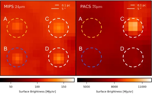
Fig. 2.— A patch of the CMZ observed by MIPS 24µm (left)
and PACS 70µm (right). The real object (A) is marked with a
yellow dashed circle, the syntheticStage 2+source (B) by a blue
circle and the two synthetic Stage 0/1sources (C, D) by white
circles. In MIPS 24µm the synthetic observations shown agree with
the real observation. The synthetic Stage 2+source as well as
the lower syntheticStage 0/1source agree with the PACS 70µm
observation of the real source.
3. RESULTS
3.1. Real observations vs. realistic synthetic
observations
In this section, we compare three model objects, as described in Section 2, added to observations to com-pare to a real source classified as a YSO. In Figure 2we placed three synthetic observations (A0 Stage 2+, B5 and B8 Stage 0/1) next to a classified YSO of Stage 0/1 by Yusef-Zadeh et al. (2009) at equatorial coordi-nates αJ2000 = 17h44m26.835s, δJ2000 = −29◦15′21.05′′ (yellow circle), which is clearly visible in MIPS 24µm, but with no counterpart in the Herschel observations.
Our radiative transfer model of an embedded B5 YSO of Stage 0/1 with ˙M = 3×10⁻⁴M
⊙yr−1 (C: upper white circle) matches the real object in MIPS 24µm (A: yellow circle), but also produces a source detected in PACS 70µm. On the other hand, the B8 Stage 0/1 model with ˙M = 10−4M
⊙yr−1 (D: lower white circle) has only a hardly detectable counterpart in PACS 70µm, while matching the MIPS observation. Our model of a more evolved source, an A0 Stage 2+ with ˙M = 3 ×10⁻⁷M
Wavelength λ [µm] 10-8 10-9 10-10 10-11 10-12 10-13 Flu x λFλ [ ergs /s /cm 2] without extinction no PAH dust
Wavelength λ [µm] 10-8 10-9 10-10 10-11 10-12 10-13 Flu x λFλ [ ergs /s /cm 2] with extinction no PAH dust
10-2 10-1 100 101 102 103
[image:6.612.54.300.60.328.2]Wavelength λ [µm] 10-8 10-9 10-10 10-11 10-12 10-13 Flu x λFλ [ ergs /s /cm 2] with extinction PAH dust
Fig. 3.— Evolution of the synthetic SEDs at different evolu-tionary stages of a B0 star embedded within an ambient medium
of density ρ0 = 10−21g cm−3 considering the effects of
extinc-tion and PAH dust. Vertical lines (solid: IRAC 8µm, dashed:
MIPS 24µm, dot-dashed: PACS 70µm, dotted: PACS 160µm),
SEDs from black to yellow (3×10⁻⁴M⊙yr−1, 10−4M⊙yr−1, 3×
10−5M
⊙yr−1, 10−5M⊙yr−1, 3×10⁻⁶M⊙yr−1, 10−6M⊙yr−1,
3 × 10⁻⁷M⊙yr−1, 10−7M⊙yr−1, 3 × 10⁻⁸M⊙yr−1,
main-sequence star with no envelope).
10-9 10-10 10-11 10-12 10-13 Flu x λFλ [ ergs /s /cm
2] 307175307175307175 317711317711317711317711317711317711
10-9 10-10 10-11 10-12 10-13 Flu x λFλ [ ergs /s /cm
2] 321628321628321628321628 331513331513331513
10-1 100 101 102 103
Wavelength λ [µm] 10-9 10-10 10-11 10-12 10-13 Flu x λFλ [ ergs /s /cm
2] 335380335380335380
100 101 102 103
Wavelength λ [µm] 344820
344820 344820 344820 344820
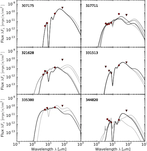
Fig. 4.— Real SEDs (circles) of six classified YSOs shown in
Figure1. The black and gray solid lines represent the synthetic
SEDs from the modeling with the best and acceptableχ2 fits,
re-spectively. The triangles represent 5σupper limits in PACS 70µm
(and for object 331513 also in the IRAC bands).
explained by both Stage 0/1 and Stage 2+ models, and so may not be as young as 1 Myr.
3.2. Evolution in the Spectral Energy Distribution
In Figure 3, we show the evolution in the SED of a B0 star from deeply embedded to main sequence object, for three dust configurations: with regular dust and no extinction; with regular dust and extinction; and with PAH dust and extinction. Naturally, the extinction af-fects more strongly the near-infrared (NIR) bands. The PAHs add emission features in the mid-infrared (MIR), but does not change too much above 24µm. The far-infrared (FIR) remains almost unaffected by both ex-tinction and PAH dust emission.
Below we describe the evolution of the SED as a func-tion of evolufunc-tionary stage. The evolufunc-tion of the SED from a main sequence source to a deeply embedded ob-jects is best observed for regular dust and extinction (middle panel of Figure 3). For a main-sequence ob-ject (with no envelope, yellow line), which is surrounded by an ambient medium, most of the mass is located at larger radii where the temperature is cold, and the mass of hotter material is low. This explains the lack of MIR emission. For the models with increasing infall rate, more material is added in the hotter regions closer to the star. As long as the dust is optically thin, the temperature of the dust in the inner regions stays constant, but the mass of the dust at these temperatures increases. The flux from this heated dust in the center is emitted in the NIR and MIR, which causes the rise at these wavelengths (e. g. infall rate 10−6M
⊙yr−1). NIR photons escape the system since the probability of re-absorption is too small. A higher accretion rate increases the envelope density, and the envelope starts to become optically thick to the stellar radiation at optical wavelengths. The tempera-ture in the outer regions drops, resulting in a drop in the FIR emission. The emission in NIR and MIR goes down, once the envelope is also no longer optically thin at that wavelength (see infall rate>3×10⁻⁶M
⊙yr−1), and the FIR emission rises again due to the absorbed radiation getting re-emitted.
For the six classified YSOs in the panels of Figure 1 we now plot the measured SEDs in Figure 4. We used the available IRAC fluxes published in the point-source catalog ofRam´ırez et al.(2008), and extracted the MIPS 24µm from the point-source catalog provided by Hinz et al. (2009). These measured fluxes were the same as used byYusef-Zadeh et al.(2009). We computed the 5σ
upper limits for PACS 70µm (triangles) after removing the background. We assumed an average error of 10 % in the fluxes as used byRobitaille et al.(2007). The black solid line shows the best fitχ2bestwith the lowestχ
2. The
grey solid lines represent the synthetic model SEDs for which (χ2−χ2
[image:6.612.53.301.426.680.2]Fig. 5.—MIPS 24µm radial brightness profiles after convolution with the PSF (shown as the dashed line). a) main-sequence objects
without cirumstellar material, ambient medium gas density ρ0 = 1×10⁻²¹g cm−3, no PAH dust b) B0 main-sequence star without
cirumstellar material but with varying ambient mediumρ0 c) B0 star with various infall rates embedded in an ambient medium with gas
densityρ0= 1×10⁻²¹g cm−3, no PAH dust. Models with hotter central stars and less dense circumstellar or ambient medium are more
resolved that models with cooler central objects and/or models with denser circumstellar and/or ambient medium.
originate from an unrelated foreground object. Objects 317711, 321628, 335380 and 344820 can be either fitted byStage 0/1orStage 2+objects of spectral type B5, B8, A0, A5 and B8, B5, A0, respectively. Hence, that SED fitting alone can not be used to distinguish between true YSOs and more evolved objects.
3.3. Evolution in the radial profiles
By inspecting the YSOs classified byYusef-Zadeh et al. (2009) in the 24µm images, we found that some ob-jects appear to be resolved, i. e. some sources are slightly larger than point sources. Therefore, we explore the ra-dial brightness profiles of our synthetic images in MIPS 24µm.
In Figure5, a compilation of normalized profiles of the realistic synthetic observations are shown. The dashed line represents the PSF of a perfect point source. Its full-width-half-maximum (FWHM) is roughly 6′′. Without an envelope (Figure 5a) the sources become more ex-tended for higher temperature stars. The low density of the surrounding medium enhances this effect (Fig-ure5b), while the presence of circumstellar dust reduces the width of the profile (Figure 5c). Resolved sources could therefore be earlier type stars and/or stars embed-ded in a low density environment (either circumstellar and/or ambient medium).
3.4. Distinguishing embedded YSOs from more evolved
objects
In this Section, based on the observational properties of our models such as MIPS 24µm magnitude, MIPS 24µm angular size and MIR color, we explore how to distinguish between true YSOs (Stage 0/1) from more evolved objects (Stage 2+) in the CMZ.
3.4.1. Detection in MIPS 24µm and PACS 70µm
Using the source counts as a function of magnitude of the point source catalogues, we determined approximate detection limits for the western part of the CMZ, where most of the YSOs classified byYusef-Zadeh et al.(2009) are located. For UKIDSS K, IRAC 8µm and MIPS 24µm we found, respectively, upper limits of 14.8 mag, 8.9 mag and 6.0 mag for a completeness of 90 %, and 15.5
5 0 5 10 15
MIPS 24µm [mag] 100
101
102
103
104
105
106
Ma
xim
um
Su
rfa
ce
Br
igh
tne
ss
at
PAC
S 7
0
µm
[M
Jy/
sr]
5σ detection
1σ detection
MI
PS
24
µm
up
pe
r li
mi
t
10−8 10−7 10−6 10−5 10−4
MS pre MS stars with envelopes
O5 O6 O8 B0 B1 B2 B3 B5 B8 A0 A5 (pre) MS stars
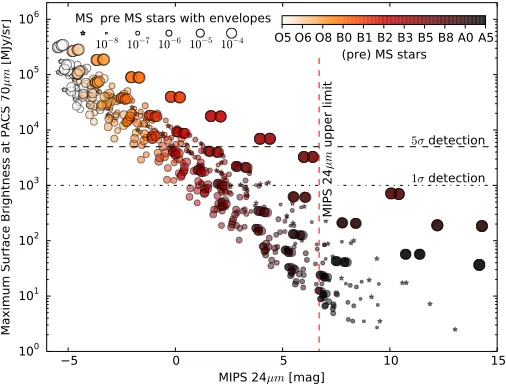
Fig. 6.—PACS 70µm peak surface brightness and MIPS 24µm magnitudes for all the models, color coded by spectral type. The detection limits of HiGal and MIPSGal in the CMZ are shown as horizontal and vertical lines.
mag, 9.8 mag and 6.7 mag for a completeness of 50 %, within an error of about 0.25 mag, which is the bin width used to construct the magnitude histograms. For PACS 70µm we estimated a 5σsurface brightness detection to be at roughly 5000 MJy/sr. In Figure 6, we show the PACS 70µm peak surface brightness versus the MIPS 24µm magnitude for the 660 modelled objects, indicat-ing the different spectral types and envelope infall rates. A total of 567 model objects can be detected in MIPS 24µm as indicated by the vertical dashed line in Fig-ure6. The MIPS 24µm detection limit corresponds to a completeness limit of B5 in spectral type. On the other hand, the PACS 70µm 5σdetection limit (also shown in Figure 6) translates into a completeness limit of O8 in spectral type, but also some evolutionary stages of B0 to B3 objects can be 5σ-detected in PACS 70µm, while later types show no 5σ-detected counterparts.
[image:7.612.317.570.285.477.2]-5 0 5 10 15 MIPS 24µm [mag]
100
101
102
103
104
105
106
Ma
xim
um
Su
rfa
ce
Br
igh
tne
ss
at
PAC
S 7
0
µm
[M
Jy/
sr] a)
5σ detection
1σ detection
MIPS
24
µm
up
pe
r li
mi
t
10−8 10−7 10−6 10−5 10−4
MS pre MS stars with envelopes evolutionary stage 0/1 2+
3.0 3.5 4.0 4.5 5.0 5.5
MIPS 24µm Half-Width-Half-Maximum [arcsec] 5
0
5
10
15
MIPS
24
µm
[m
ag
]
b)
PS
F M
IPS
24
µm
Criteria I
MIPS 24µm upper limit
10−8 10−7 10−6 10−5 10−4
MS pre MS stars with envelopes evolutionary stage 0/1 2+
0 2 4 6 8
IRAC 8µm - MIPS 24µm [mag] 5
0
5
10
MIPS
24
µm
[m
ag
]
c)
upper limit MIPS 24µm
Yusef-Zadeh et al. (2009) Criteria II
upper limit IR AC 8µm
10−8 10−7 10−6 10−5 10−4
MS pre MS with envelopes evolutionary stage
MIPS resolved 0/1 2+
0 2 4 6 8 10
IRAC 8µm - MIPS 24µm [mag] 0
5
10
15
20
25
UKIDSS K [mag]
d)
upper limit UKIDSS K
Criteria II
10−8 10−7 10−6 10−5 10−4
MS pre MS with envelopes evolutionary stage
[image:8.612.54.562.59.460.2]MIPS resolved 0/1 2+
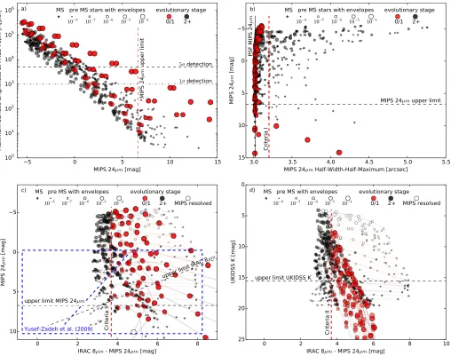
Fig. 7.—Diagnostic diagrams extracted from our synthetic observations: a) Peak PACS 70µm surface brightness vs. and MIPS 24µm
magnitude diagram. The red line shows the MIPS 24µm and the black lines show the PACS 70µm detection limits. b) MIPS 24µm
HWHM vs. MIPS 24µm. Red dashed line shows our criteria to distinguish between resolved and unresolved objects, black dashed line is
the MIPS 24µm upper limit. c) Color-magnitude diagram in the MIR. The blue dashed box represents the plotting limits ofYusef-Zadeh
et al.(2009), blue dashed diagonal line is the empirical criteria byYusef-Zadeh et al.(2009) to distinguish AGB stars from YSOs. Black
dashed lines are upper limits in MIPS 24µm and IRAC 8µm. The red vertical dashed line separates more evolved objects from the sample.
d) Color-magnitude diagram MIR vs. NIR. The black dashed line is upper limit in UKIDSS K. The red vertical dashed line separates more
evolved objects from the sample. (red: Stage 0/1, black:Stage 2+, white: MIPS resolved)
detection limit in PACS 70µm. Therefore, detection or non-detection of sources at PACS 70µm does not allow us distinguish true YSOs from more evolved objects in the CMZ, disproving the hypothesis put forward in Sec-tion 1 that objects only seen at MIPS 24µm and not detected at PACS 70µm would not be YSOs.
3.4.2. Half-width-half-maximum in MIPS 24µm
To explore the effects in the radial profiles described in Section 3.3, we need the half-width-half-maximum (HWHM) of all models in MIPS 24µm. We devel-oped a tool which can fit PSF models for extended sources, which consist of Gaussian profiles convolved with the MIPS 24µm PSF. The fit can be carried out manually in order to ensure an optimal fit in regions of complex background. The profile with the best fit is used to calculate the ‘observed’ HWHM, which is roughly
q
HWHM2P SF+ HWHM2Gauss. We fit the
syn-thetic sources with 100 profiles with combined HWHMs ranging from 3 to 6′′(1 HWHM to 2 HWHM). With this PSF fitting method it was also possible to extract total integrated fluxes. In Section3.5we use this technique on real observations.
In Figure 7b, we plot the MIPS 24µm magnitude vs. the MIPS 24µm HWHM. About half of the objects lie exactly on the PSF (HWHM = 3.02′′) and are therefore unresolved. We find that most resolved objects are have an inverse timescale ˙Mgas/M⋆ less than 10−6yr−1 and are therefore not likely to be as young as assumed by e. g.Yusef-Zadeh et al. (2009).
We adopt the Stage formalism to explore whether the objects in the vicinity of the PSF can be disentangled. We found that 228 of the 660 model objects are in fact still in the envelope dominated phase (Stage 0/1). We define a HWHM threshold of 3.2′′ to separate
re-solved objects (HWHM ≥3.2′′) from
(HWHM <3.2′′). There are only nine resolved Stage
0/1 model objects, and these are all below the MIPS 24m detection limit. Therefore, most of the resolved ob-jects (165 of 174) are more evolvedStage 2+. A total of 486 objects are unresolved and include objects from both Stages of evolution (219 Stage 0/1, 267 Stage 2+). Note that while seeing an extended source at 24µm likely indicates that a source is not truly young, unre-solved sources can still be ambiguous.
3.4.3. MIR and NIR color-magnitude diagrams
In what follows, we now have a closer look at the 481 unresolved model objects using color-magnitude di-agrams, in order to understand to what extend we can distinguish between embedded YSOs from more evolved objects. Figure7cpresents the IRAC 8µm - MIPS 24µm vs. MIPS 24µm color-magnitude diagram. Yusef-Zadeh et al.(2009) used an empirical criterion (see blue dashed diagonal line in Figure7c) to distinguish AGB field stars from YSOs. Our modelling shows that this criterion alone (without accounting for resolved and unresolved objects) is not effective to separate true YSOs from more evolved objects, since these overlap in color-magnitude space. The evolutionary tracks in the color-magnitude diagram can be explained similarly to the SED evolution described in Section 3.2. Although there is some over-lap, sources with IRAC 8µm - MIPS 24µm < 3.7 mag are always more evolved.
One can see that the MIR color-magnitude diagram alone (without accounting for resolved and unresolved objects) is not capable to completely distinguish between more evolved and deeply embedded YSOs. Combining bands in the NIR and the MIR seems more promising if the detection in K is sensitive enough, as can be noted in Figure7d, which shows the IRAC 8µm - MIPS 24µm vs. UKIDSS K color-magnitude diagram. The K band is dominated by stellar emission that is simply extincted, so it directly probes the envelope column density. Since the column density is very different between the main-sequence stars and ambient medium compared to with envelopes, all envelope dominated objects fall in one dis-tinctive region in the diagram.
3.4.4. Criteria to select true YSOs
In summary, we have shown that the following criteria can be used to preferentially select truly young Stage 0/1 YSOs, based on the MIPS 24µm size and IRAC 8µm - MIPS 24µm color:
I MIPS 24µm HWHM<3.2′′
II IRAC 8µm - MIPS 24µm>3.7 mag
Of the 660 model objects, 343 match these criteria. Of these, 219 are true YSOs models and instead of however 124 are models of more evolved objects. Nine objects are misclassified as more evolved but are true YSOs and lie below the MIPS 24µm detection limit. The remaining 308 are all models of more evolved objects. In summary, using these criteria on our models results in:
33.2 % correctly classified Stage 0/1objects 46.7 % correctly classified Stage 2+objects 18.8 % misclassified as Stage 0/1
1.4 % misclassified asStage 2+
3.0 3.5 4.0 4.5 5.0 5.5 6.0
MIPS 24µm Half-Width-Half-Maximum [arcsec] 0
2
4
6
8
10
MI
PS
24
µm
[m
ag
]
Fig. 1
PS
F M
IPS
24
µm
Criteria I
MIPS 24µm upper limit
good multiple
Fig. 8.—Observation counterpart to Figure7b. Measured sizes of sample points of good quality (blue circles) and others which
appear to be multiple sources (white triangles) from the
Yusef-Zadeh et al.(2009) sample. The sample sources of bad quality are not included. Points with white stars surrounded by blue circles
represent the measurements of the six objects showed in Figure1.
When including protoplanetary disks (rmax = 1000 AU) to our YSO circumstellar geometry setup the above criteria are mostly unchanged. Overall models with discs are slightly less extended due to the increased mass of circumstellar material in the center. Therefore, the selection criteria I in MIPS 24µm is not quite as suc-cessful as for the runs without disks. For models with a disk, the classification fractions are as follows:
33.2 % correctly classifiedStage 0/1objects 33.3 % correctly classifiedStage 2+objects 32.1 % misclassified asStage 0/1
1.4 % misclassified asStage 2+
3.5. Correcting previously estimated SFR
With these criteria it is possible to revise SFR calcu-lations from the literature. Here we investigate the 213 sources classified as Stage 0/1 by Yusef-Zadeh et al. (2009). We use the PSF fitting tool described in Sec-tion 3.4.2with 20 extended models with total HWHMs ranging from 3 to 6′′. We used fewer profiles than for synthetic observations, because for real observations the fitting is done by hand. The measuring tool is robust to distinguish between unresolved and resolved objects. The error increases with increasing size in real observa-tions, but sizes smaller than HWHM <3.5′′ appear to be robust. We also estimate the total flux of the objects. The values of the magnitudes suffer from errors depend-ing on the background. In Figure8we plot our measured sizes and magnitudes.
By visually inspecting the MIPS 24µm images, we noted first that about 31.0 % of the sources are likely unreliable, of which 56 % correspond to parts of diffuse emission erroneously fitted as point sources in the orig-inal catalogue and 44 % of the sources show evidence of multiplicity.
thresh-old of 3.2′′, 49.3 % of the objects have a larger HWHM, but this may include objects that appear to be larger due to noise, so that this value should be treated more cautiously. This means that at least 63.4 % (32.4 % + 31.0 %) and maybe 80.3 % (49.3% + 31.0 %) or more of theYusef-Zadeh et al.(2009) sources may therefore not be YSOs, lowering the star formation rate by a factor of three or more and bringing it closer to the value of the SFR estimated from free-free emission (seeLongmore et al. 2013).
Given the issues with spurious sources mentioned above, a careful characterization of each source at MIPS 24µm and IRAC 8µm is therefore needed in future to pin down the SFR in the CMZ more accurately.
4. DISCUSSION
Our “realistic synthetic observations” from radiative transfer modelling (see Section2) have shown that more evolved objects (i. e. main-sequence stars) in a low-density ambient low-density medium could mimic YSOs, for all spectral types discussed in this paper. We found that Stage 2+ objects with spectral types later than B3, detected in MIPS 24µm, are predicted to have no 5σ -observable counterpart in PACS 70µm, similar to some of the objects classified as YSOs by Yusef-Zadeh et al. (2009).
Unresolved MIPS 24µm sources could be heavily em-bedded objects (Stage 0/1) or more evolvedStage 2+, while resolved objects are most likely Stage 2+ ob-jects. This means that resolved model objects detected in MIPS 24µm in the CMZ are more evolved and there-fore likely older than 1 Myr. All these arguments that indicate some objects classified in the CMZ are not very young embedded YSOs (i. e. less than 1 Myr) as previ-ously thought. Therefore, the star formation rate of 0.14 M⊙yr−1 (Yusef-Zadeh et al. 2009) is likely over-estimated.
4.1. Stellar distribution from the IMF
To get an idea of how many main-sequence stars of var-ious spectral types should be in the CMZ, we performed simple estimations using aKroupa (2001) IMF. Assum-ing a constant SFR of 0.01 M⊙yr−1(seeLongmore et al.
2013), roughly four O stars and 5183 B stars (including and earlier than B5) should be at the distance of the CMZ. We note, that in this IMF calculation the ages of the stars are equally distributed. Since the lifetime of a MIPS 24µm detectable B star lies, as mass decreases (B0 to B5, M∈[17.5,5.9] M⊙), between 8 Myr and 113 Myr, only a few objects should be primordial (Stage 0/1, smaller than 1 Myr), while the majority would be in the main-sequence phase (Stage 2+). Not necessarily, all 5138 B stars (including and earlier than B5) could be observed in MIPS 24µm, since sources in lower ambi-ent densities environmambi-ents can not produce strong MIR emission in order to be detected.
4.2. Origin of the main-sequence stars
In the CMZ there are many objects with MIPS 24µm emission west from the Galactic center, which appear not to be part of an active star-forming region analogous to Sgr B2 or Sgr C. Our results show, that some of those may be in fact more evolved objects (i. e. main-sequence stars) and not true YSOs.
However, more evolved objects with ages of several Myr will not have formed at the observed spot. One could envisage a scenario in which an OB association formed at the current location of Sgr B2, then got dis-rupted at a later time while orbiting the Galactic cen-ter. For example, an object observed at 41.6′ or 103 pc from the Galactic center with an average orbital speed of about 140 km s−1 (Sofue 2013) has an orbital time-scale of 4.5 Myr, thus all more evolved objects with spectral types earlier than B5 will have completed at least one orbit around the Galactic centre since their birth.
4.3. Giants in the CMZ
It is also possible that giants could mimic YSOs. An et al.(2011) found that there are supergiants in the CMZ. Evolved objects like supergiants should not produce HII regions. There is not a large overlap with the Yusef-Zadeh et al.(2009) sample of YSOs but still when recal-culating the SFR one should consider these objects, be-cause contamination of the sample would overestimate the SFR. We produced synthetic observation of super-giants3 from spectral type B0 to M0 and found that they are distributed amongst resolved sources and could be therefore also be removed by our selection criteria. Further, in the NIR/ MIR color space (e. g. Figure 7d) most supergiants are redder thanStage 0/1sources but brighter than 12 mag in K band and 8 mag in IRAC 8µm, and therefore would be easily distinguishable in color space.
4.4. Predictions for high-resolution mm observations
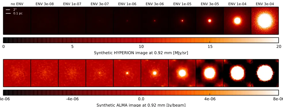
We now briefly describe whether high-resolution mm observations could help us to distinguish between the main-sequence stars (Stage 2+) and true YSOs (Stage 0/1). In particular, one would expect that the YSOs will show much more dense dust/ gas in the central regions. Millimetre observations of reclassified Stage 0/1 and Stage 2+ sources could help us to constrain our pre-dictions, and reduce the number of Stage 2+ objects misclassified as YSOs. In Figure 9, our 0.9 mm predic-tion of ALMA observapredic-tions using Hyperion andCasa
of a B5 star3at all evolutionary stages is presented (dust continuum with a bandwidth of 7.5 GHz, total observ-ing time 1200 s, beam size ∼ 0.5 ′′). The four models to the right with the highest infall rate are Stage 0/1 sources. Stage 0/1objects are much brighter and have much more flux on the small scales, while for the most evolved ones, there is very little dense material so most of the emission is extended or not detected. Our analy-sis of the synthetic ALMA images show that it would be possible to use mm observations to distinguish between the main-sequence stars and the YSOs.
5. SUMMARY
With our realistic synthetic observation from radiative transfer modeling, we have shown that some of the classi-fied YSOs (Yusef-Zadeh et al. 2009) in the CMZ may not necessarily be as young as previously thought (i. e. less then 1 Myr). In addition, we have shown that some of the observed objects can be better explained by more evolved objects such as main-sequence stars in a constant density interstellar medium. We found that:
Fig. 9.—Millimeter observation observed through a perfect interferometer of a B5 star (top) and synthetic ALMA observations (bottom).
True YSO (Stage 0/1) model objects are much brighter and have much more flux on the small scales, while for the most evolved ones,
there is very little dense material so most of the emission is extended or not detected. Six models from the left: Stage 2+, four models
from the right: Stage 0/1.
• detection/ non-detection in PACS 70µm is not a reliable handle to distinguish true YSOs from more evolved objects.
• resolved, extended objects in MIPS 24µm are un-likely to be deeply embedded YSOs and therefore not truly young.
These findings lead us to believe that the SFR in the CMZ estimated by directly counting YSOs (Yusef-Zadeh et al. 2009) is over-estimated by at least a factor of three (and potentially up to a factor of 5). A lower SFR for the CMZ would be in better agreement with estimates from free-free emission (e. g.Longmore et al. 2013). By producing synthetic observations of our YSO models, we have shown that high resolution dust continuum
observa-tions with ALMA could in future help to provide a more definite classification of the YSO candidates.
ACKNOWLEDGEMENT
We thank the referee for a constructive report that helped us improve the clarity and the strength of the results presented in our paper. This work was partially carried out in the Max Planck Research GroupStar
for-mation throughout the Milky Way Galaxy at the Max
Planck Institute for Astronomy. C. K. is a fellow of the International Max Planck Research School for Astron-omy and Cosmic Physics (IMPRS) at the University of Heidelberg, Germany and acknowledges support.
REFERENCES
An, D., Ram´ırez, S. V., Sellgren, K., et al. 2011, ApJ, 736, 133 Aniano, G., Draine, B. T., Gordon, K. D., & Sandstrom, K. 2011,
PASP, 123, 1218
Benjamin, R. A., Churchwell, E., Babler, B. L., et al. 2003, PASP, 115, 953
Calzetti, D. 2013, Star Formation Rate Indicators, ed.
J. Falc´on-Barroso & J. H. Knapen, 419
Carey, S. J., Noriega-Crespo, A., Mizuno, D. R., et al. 2009, PASP, 121, 76
Carroll, B. W., & Ostlie, D. A. 1996, An Introduction to Modern Astrophysics (Addison Wesley Publishing Company)
Castelli, F., & Kurucz, R. L. 2004, ArXiv Astrophysics e-prints, astro-ph/0405087
Chomiuk, L., & Povich, M. S. 2011, AJ, 142, 197
Churchwell, E., Babler, B. L., Meade, M. R., et al. 2009, PASP, 121, 213
Draine, B. T. 2003, ARA&A, 41, 241 Draine, B. T., & Li, A. 2007, ApJ, 657, 810
Evans, II, N. J., Dunham, M. M., Jørgensen, J. K., et al. 2009, ApJS, 181, 321
Geballe, T. R., Najarro, F., Figer, D. F., Schlegelmilch, B. W., & de La Fuente, D. 2011, Nature, 479, 200
Hewett, P. C., Warren, S. J., Leggett, S. K., & Hodgkin, S. T. 2006, MNRAS, 367, 454
Hinz, J. L., Rieke, G. H., Yusef-Zadeh, F., et al. 2009, ApJS, 181, 227
Kim, S.-H., Martin, P. G., & Hendry, P. D. 1994, ApJ, 422, 164 Kroupa, P. 2001, MNRAS, 322, 231
Longmore, S. N., Bally, J., Testi, L., et al. 2013, MNRAS, 429, 987
Lucas, P. W., Hoare, M. G., Longmore, A., et al. 2008, MNRAS, 391, 136
Lutz, D., Feuchtgruber, H., Genzel, R., et al. 1996, A&A, 315, L269
Molinari, S., Swinyard, B., Bally, J., et al. 2010, PASP, 122, 314 Molinari, S., Bally, J., Noriega-Crespo, A., et al. 2011, ApJ, 735,
L33
Quijada, M. A., Marx, C. T., Arendt, R. G., & Moseley, S. H. 2004, in Society of Photo-Optical Instrumentation Engineers (SPIE) Conference Series, Vol. 5487, Society of Photo-Optical Instrumentation Engineers (SPIE) Conference Series, ed. J. C. Mather, 244–252
Ram´ırez, S. V., Arendt, R. G., Sellgren, K., et al. 2008, ApJS, 175, 147
Robitaille, T. P. 2011, A&A, 536, A79
Robitaille, T. P., Churchwell, E., Benjamin, R. A., et al. 2012, A&A, 545, A39
Robitaille, T. P., & Whitney, B. A. 2010, ApJ, 710, L11 Robitaille, T. P., Whitney, B. A., Indebetouw, R., & Wood, K.
2007, ApJS, 169, 328
Robitaille, T. P., Whitney, B. A., Indebetouw, R., Wood, K., & Denzmore, P. 2006, ApJS, 167, 256
Sofue, Y. 2013, PASJ, 65, 118 Ulrich, R. K. 1976, ApJ, 210, 377
Weingartner, J. C., & Draine, B. T. 2001, ApJ, 548, 296 Whitney, B. A., Robitaille, T. P., Bjorkman, J. E., et al. 2013,
ApJS, 207, 30
APPENDIX
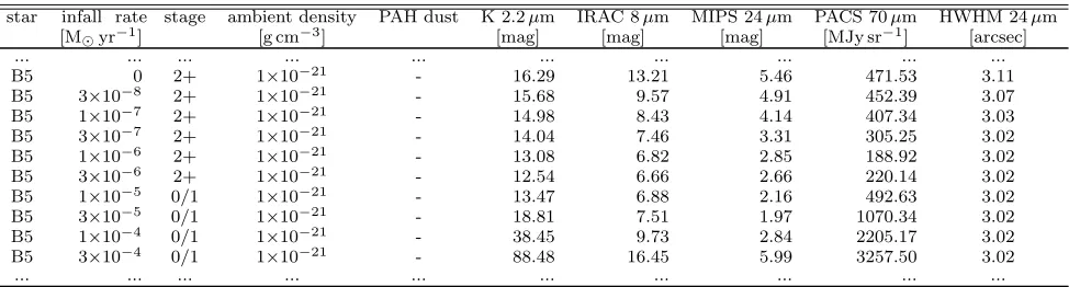
[image:12.612.64.551.174.305.2]Here we present input (spectral type, envelope infall rate, stage, ambient medium, dust type) and output (magnitude in UKIDSS 2.2µm, IRAC 8µm and MIPS 24µm and the maximum surface brightness in PACS 70µm, MIPS 24µm HWHM) parameters of the 660 models of YSOs and main-sequence stars in an ambient density environment as well as the models of the supergiants.
TABLE 3
Parameters and measurements from our models.
star infall rate stage ambient density PAH dust K 2.2µm IRAC 8µm MIPS 24µm PACS 70µm HWHM 24µm
[M⊙yr−1] [g cm−3] [mag] [mag] [mag] [MJy sr−1] [arcsec]
... ... ... ... ... ... ... ... ... ...
B5 0 2+ 1×10⁻²¹ - 16.29 13.21 5.46 471.53 3.11
B5 3×10⁻⁸ 2+ 1×10⁻²¹ - 15.68 9.57 4.91 452.39 3.07
B5 1×10⁻⁷ 2+ 1×10⁻²¹ - 14.98 8.43 4.14 407.34 3.03
B5 3×10⁻⁷ 2+ 1×10⁻²¹ - 14.04 7.46 3.31 305.25 3.02
B5 1×10⁻⁶ 2+ 1×10⁻²¹ - 13.08 6.82 2.85 188.92 3.02
B5 3×10⁻⁶ 2+ 1×10⁻²¹ - 12.54 6.66 2.66 220.14 3.02
B5 1×10⁻⁵ 0/1 1×10⁻²¹ - 13.47 6.88 2.16 492.63 3.02
B5 3×10⁻⁵ 0/1 1×10⁻²¹ - 18.81 7.51 1.97 1070.34 3.02
B5 1×10⁻⁴ 0/1 1×10⁻²¹ - 38.45 9.73 2.84 2205.17 3.02
B5 3×10⁻⁴ 0/1 1×10⁻²¹ - 88.48 16.45 5.99 3257.50 3.02
... ... ... ... ... ... ... ... ... ...