The relationship between well-being and commuting revisited: does the choice of methodology matter?

promoting access to White Rose research papers

White Rose Research Online

[email protected]

Universities of Leeds, Sheffield and York

http://eprints.whiterose.ac.uk/

This is a copy of the final published version of a paper published via gold open access

in

Regional Science and Economics

.

This open access article is distributed under the terms of the Creative Commons

Attribution Licence (

http://creativecommons.org/licenses/by/3.0

), which permits

unrestricted use, distribution, and reproduction in any medium, provided the

original work is properly cited.

White Rose Research Online URL for this paper:

http://eprints.whiterose.ac.uk/81608

Published paper

Dickerson, A.P., Hole, A. and Munford, L. (2014) The relationship between

well-being and commuting revisited: does the choice of methodology matter? Regional

Science and Urban Economics, 49. pp. 321-329. Doi:

The relationship between well-being and commuting revisited: Does the

choice of methodology matter?

☆

Andy Dickerson, Arne Risa Hole

⁎

, Luke A. Munford

University of Sheffield, Department of Economics, 9 Mappin Street, Sheffield S1 4DT, UK

a b s t r a c t

a r t i c l e i n f o

Article history:

Received 25 April 2013

Received in revised form 15 May 2014 Accepted 24 September 2014 Available online 2 October 2014

JEL codes:

C25 D12 I10 R41

Keywords:

Well-being Commuting Fixed-effects

This paper provides an assessment of a range of alternative estimators forfixed-effects ordered models in the context of estimating the relationship between subjective well-being and commuting behaviour. In contrast to previous papers in the literature wefind no evidence that longer commutes are associated with lower levels of subjective well-being, in general. From a methodological point of view our results support earlierfindings that linear and orderedfixed-effects models of life satisfaction give similar results. However, we argue that ordered models are more appropriate as they are theoretically preferable, straightforward to implement and lead to easily interpretable results.

© 2014 The Authors. Published by Elsevier B.V. This is an open access article under the CC-BY license (http://creativecommons.org/licenses/by/3.0/).

1. Introduction

Measures of subjective well-being are increasingly used as a proxy for individual welfare in applied economics. Summaries and overviews of this rapidly expanding literature include:Frey and Stutzer (2002a,b),

Layard (2005),Kahneman and Krueger (2006),Di Tella and MacCulloch (2006),Clark et al. (2008),Dolan et al. (2008),Stutzer and Frey (2010)

andMacKerron (2012). Survey respondents are typically asked a question like‘How satisfied are you with your life overall?’and asked to give a response on a Likert scale with the lowest and highest values corresponding to_‘Not satis_fied_’and_‘Completely satis_fied_’, respectively. Econometrically this raises the question of how to model this type of data. Since well-being as a proxy for individual welfare or utility is strictly speaking an ordinal rather than a cardinal measure_–a 1-point increase from 2 to 3 on the well-being scale may not imply the same increase in well-being as an increase from 6 to 7, for example–the stan-dard econometric approach would be to use an ordered logit or probit

model. However, in an influential paper, Ferrer-i-Carbonell and Frijters (2004)compare the results from a linearfixed-effects (FE) model, and thus implicitly treating well-being as a cardinal measure, with those from their FE ordered logit specification, andfind that they obtain similar results. An equivalentfinding has been documented by

Frey and Stutzer (2000). This has led authors in several subsequent studies to analyse their data using linear models (e.g.Stutzer and Frey (2008)), presumably because linear FE models are considered to be more straightforward to implement in practice and lead to more easily interpretable results than ordered FE models. More recently, however,

Baetschmann et al. (2011)have shown that the FE ordered logit estima-tor used in theFerrer-i-Carbonell and Frijters (2004)comparison is, in fact, inconsistent. Hence, the similarity between the linear FE and the ordered FE results is not particularly informative.

In this paper we revisit the debate surrounding the appropriate methodology for modelling subjective well-being data in the context of the relationship between commuting and well-being. According to microeconomic theory, individuals would not choose to have a longer commute unless they were compensated for it in some way, either in the form of improved job characteristics (including pay) or better hous-ing prospects (Stutzer and Frey, 2008). Even if commuting in itself is detrimental to well-being we would therefore not expect individuals with longer commutes to report lower levels of life satisfaction. As far as we are aware,Stutzer and Frey (2008)andRoberts et al. (2011)are the only previous papers that attempt to test this hypothesis by model-ling the relationship between commuting and subjective well-being.

☆ We are grateful to the Data Archive at the University of Essex for supplying the data from the British Household Panel Survey. We thank Stephen Hall, Anita Ratcliffe, Jenny Roberts, Sandy Tubeuf, Aki Tsuchiya, participants at the 2012 Health Econometrics work-shop in Siena and the 2nd Applied Health Econometrics Symposium in Leeds and seminar participants at Loughborough, Toulouse and Sheffield for valuable comments and advice. Luke Munford is grateful to the UKTRC for a Studentship.

⁎ Corresponding author. Tel.: +44 114 222 3411.

E-mail addresses:a.p.dickerson@sheffield.ac.uk(A. Dickerson),

a.r.hole@sheffield.ac.uk(A.R. Hole),ecp10lam@sheffield.ac.uk(L.A. Munford).

http://dx.doi.org/10.1016/j.regsciurbeco.2014.09.004

0166-0462/© 2014 The Authors. Published by Elsevier B.V. This is an open access article under the CC-BY license (http://creativecommons.org/licenses/by/3.0/).

Contents lists available atScienceDirect

Regional Science and Urban Economics

Using data from the German Socio-Economic Panel (GSOEP),Stutzer and Frey (2008)estimate linear FE models in which satisfaction with life overall (measured on a scale from 1 to 10) is speci_fied as a function of commuting time and a set of control variables. The authorsfind that a one standard deviation (18 min) increase in commuting time lowers re-ported satisfaction with life overall by 0.086. To put this estimate into contextStutzer and Frey (2008)report that it is equivalent to about 1/8 of the effect on well-being of becoming unemployed. The authors conclude that commuting is a stressful activity which does not pay off, a result which they refer to as the‘commuting paradox’

as it does not correspond to the predictions from microeconomic theory.

Using data from the British Household Panel Survey (BHPS),Roberts et al. (2011)model the relationship between well-being, commuting times and other personal and household characteristics. Well-being is measured by the GHQ (General Health Questionnaire) score, which is derived as the sum of the responses to 12 questions related to mental health. Using linear FE models, the authorsfind that longer commutes are associated with lower levels of subjective well-being among women but not among men. They suggest that this is likely to be a result of women having greater responsibilities for day-to-day household tasks, such as childcare and housework, and that this makes them more sensitive to longer commuting times. The authors of both papers acknowledge that the dependent variable in their models is categorical, but justify the use of a linear model based on thefindings in the study by

Ferrer-i-Carbonell and Frijters (2004).

While there is limited empirical evidence on the relationship between commuting and well-being, there is a substantial body of work on commuting in the urban economics literature with recent con-tributions includingvan Ommeren and Gutiérrez-i-Puigarnau (2011),

Ross and Zenou (2008) and Pierrard (2008). For example, van Ommeren and Gutiérrez-i-Puigarnau (2011)examine the impact of commuting on workers' productivity as manifested through higher levels of absenteeism for those with longer commutes. Theyfind evi-dence consistent with this hypothesis for Germany using the German Socio-Economic Panel. Their work builds on earlier research byRoss and Zenou (2008)whofind a positive relationship between commuting and both unemployment and wages using the US Public Use Microdata Sample from the 2000 Decennial Census, at least for more highly supervised occupations. Thesefindings are consistent with their urban efficiency wage model. Of direct relevance to our study is the large literature devoted to estimating the value of travel time;Abrantes and Wardman (2011)present a recent meta-analysis of UK estimates. As we will demonstrate, models of well-being can provide an alternative to more traditional travel demand models for estimating the value of time spent commuting.

Using data from the British Household Panel Survey, we compare the results from linear FE models and ordered logit models with and withoutfixed-effects. Wefind that while the results from the pooled ordered logit models suggest that there is a negative relationship between longer commutes and reported satisfaction with life overall, no such relationship is found in the (linear and ordered) FE models. This confirms Ferrer-i-Carbonell and Frijters'finding that the results from linear and ordered models of subjective well-being are qualitatively similar once unobservable individualfixed-effects are controlled for. We alsofind that the choice of estimator for thefixed-effects ordered logit model has little qualitative impact on the results. However, unlike

Stutzer and Frey (2008)andRoberts et al. (2011)we do not_find evidence that commuting is related to lower levels of subjective well-being, in general. This suggests that the relationship between well-being and commuting times may depend on differences in culture (the UK vs. Germany) and the choice of well-being measure (overall life satisfaction vs. the GHQ score).

The paper is structured as follows:section2describes the economet-ric methodology,section3presents the data used in the analysis and

section4presents the modelling results.Section5concludes.

2. Methodology

In this section we brie_fly review various estimators for the FE ordered logit model that have been suggested in the literature.1_Our

starting point is a latent variable model:

yit¼x0itβþαiþεit; i¼1;…;N t¼1;…;T ð1Þ

whereyit∗is a latent measure of the well-being of individualiin periodt, xitis a (L× 1) vector of observable characteristics related to well-being

andβis a (L× 1) vector of coefficients to be estimated.αiis a time-invariant unobserved component which may be correlated withxit,

andεitis a white noise error term. We observeyitwhich is related to yit∗as follows

yit¼k if μkbyit≤μkþ1; k¼1;…;K ð2Þ

The threshold parameters,μk, are assumed to be strictly increasing in

k(μkbμk+ 1∀k) withμ1=− ∞andμK+ 1=∞. Assuming thatεitis IID

logistic, the probability of observing outcomekfor individualiat timet

is

Pr yð it¼kjxit;αiÞ ¼Λ μkþ1−x0itβ−αi

−Λ μk−x0itβ−αi

ð3Þ

whereΛ(⋅) denotes the logistic cumulative distribution function. As explained byBaetschmann et al. (2011), there are two problems with direct maximum likelihood estimation of this expression. The_first is that only the difference between the thresholds and thefixed-effect

αik =μk− αican be identified. The second is that underfixed-T

asymptoticsαikcannot be estimated consistently due to the incidental parameter problem (Neyman and Scott, 1948). This unfortunately also affects the estimates ofβ, and it has been found that the bias can be substantial in short panels (Greene, 2004).

Winkelmann and Winkelmann (1998)suggest that a way of getting around this problem is to collapseyitto a binary variable and use

Chamberlain's estimator forfixed effects binary logit models.2_Following

Baetschmann et al. (2011)we de_fine a variableditk=I(yit≥k) whereI(⋅)

is the indicator function andkis a cutoff value. In other words,ditkis

equal to one ifyitis greater than or equal to the chosen cutoff value

and zero otherwise. The probability of observing a particular sequence of outcomesdik= (dik1,…,diTk) conditional on the number of ones in

the sequence (ai) is given by

Pr dki

XT

t¼1 dkit¼ai

!

¼ exp

XT t¼1d

k itx0itβ

X

li∈Biexp

XT t¼1litx0itβ

ð4Þ

wherelitis either zero or one,li= (li1,…,liT) andBiis the set of all

possible li vectors with the same number of ones as dik.

Chamberlain (1980) shows that maximising the conditional log-likelihoodLLk_=∑

i= 1 N _ln[Pr(d

i k_|∑

t= 1

T _d

it k_=a

i)] gives a consistent

estimate ofβ.

While in principle any cutoff 2≤k≤Kcan be used in the estimation it is important to note that individuals with constantditkdo not

contrib-ute to the likelihood.3_{This implies that any particular choice of cutoff is}

likely to lead to some observations being discarded and the question is then whether we can do better than choosing a single cutoff. We will

1 _{For simplicity we omit some technical details and focus on what we believe are the}

most important practical issues. We refer interested readers to the comprehensive review byBaetschmann et al. (2011).

2

Another possible solution is to make the assumption thatαi¼x0iδþviwhereviis IID

normal with mean zero. Under this assumption the parameters in the model can be con-sistently estimated by includingxitandxias regressors in a random effect ordered logit

model. This approach, which was originally proposed byMundlak (1978)in the context of linear models, is not pursued in this paper as we prefer not to have to make this addi-tional strong assumption.

3

review three alternative estimators that have been proposed in the literature: theDas and Van Soest (1999)estimator, the‘Blow-up and Cluster' estimator (Baetschmann et al., 2011) and the Ferrer-i-Carbonell and Frijters (2004)estimator.

2.1. The Das and Van Soest (DvS) estimator

Since the estimator ofβat any cutoff β^k is consistent,Das and Van Soest (1999)proposed estimating the model using allK-1 cutoffs and combine the estimates in a second step. The efficient combination weights the estimates by their variance so that

^

βDvS¼arg min

b ^

β20−b0;…;β^K0−b0

^

Ω−1β^20−b0;…;β^K0−b00 ð5Þ

whereΩ^−1

is an estimate of the variance–covariance matrix of the coefficients. The solution to this problem is

^ βDvS

¼ H0Ω^−1 H

₋1

H0Ω^−1 _^ β20

;…;β^K0

₀

ð6Þ

whereHis a matrix ofK-1 stacked identity matrices of dimensionL. The variance–covariance matrix ofβ^DvS

is given by

Varβ^DvS

¼ H0Ω^−1 H

₋1

ð7Þ

Appendix B.1presents code for implementing the DvS estimator in Stata. The drawback of the DvS estimator is that in many real settings some cutoff values are going to lead to very small estimation samples. This may lead to convergence problems and/or imprecise estimates of the variance–covariance matrixΩ^−1, and it may therefore be necessary to use only some of the possible cutoffs when implementing the DvS estimator in practice.

2.2. The‘Blow-up and Cluster’(BUC estimator)

Baetschmann et al. (2011)have recently suggested an alternative to the DvS estimator which avoids the problem of small sample sizes asso-ciated with some cutoff values. Essentially the BUC estimator involves estimating the model using allK-1 cutoffs simultaneously, imposing the restriction thatβ2_=β3_=⋯=βK_{. In practice this can be done by}

creating a dataset where each individual is repeatedK-1 times, each time using a different cutoff to collapse the dependent variable. The model is then estimated on the expanded sample using the standard Chamberlain approach. Since some individuals contribute to several terms in the log-likelihood function it is necessary to adjust the standard errors for clustering at the level of the respondent, hence the name

‘Blow-up and Cluster’(Baetschmann et al., 2011).Appendix B.2presents code for implementing the BUC estimator in Stata with an example using simulated data.4

2.3. The Ferrer-i-Carbonell and Frijters (FF) estimator

An alternative estimator to the ones described above was proposed byFerrer-i-Carbonell and Frijters (2004). As opposed to the DvS and BUC estimators, which make use of every possible cutoff, the Ferrer-i-Carbonell and Frijters (FF) estimator involves identifying an optimal cutoff for each individual. The optimal cutoff is defined as the value

which minimises the (individual) Hessian matrix at a preliminary esti-mate ofβ. Many applied papers have instead used a computationally simpler rule for choosing the cutoff, such as the individual-level mean or median ofyit(e.g.Booth and Van Ours, 2008, 2009; Kassenboehmer

and Haisken-DeNew, 2009; Jones and Schurer, 2011).Baetschmann et al. (2011)show that FF-type estimators are in general inconsistent since the choice of cutoff is endogenous. In a simulation experiment they find that the bias in the FF estimates can in some cases be substantial, while the DvS and BUC estimators generally perform well.5 _{Code for implementing the Ferrer-i-Carbonell and Frijters}

(2004)estimator in Stata is available from the authors on request.

3. Data

This paper uses data from waves 6 to 18 (1996–2008) of the British Household Panel Survey (BHPS), a nationally representative panel sur-vey conducted by the Institute for Economic and Social Research, based at the University of Essex, UK. The households in the sample are re-interviewed on an annual basis and by wave 18 (2008), about 16,000 individuals participated in the survey. Waves 6 to 18 were chosen as they represent the only waves for which data on overall life satisfaction are available (although no data are available for wave 11 (2001) when the life satisfaction question was omitted from the survey questionnaire).

We restrict the sample to include only respondents of working age, defined to be individuals between the ages of 17 and 65 inclusive. Sim-ilarly only people who respond that they are employed are retained in the sample. Self-employed respondents are not included, since they are more likely to work from home and generally have different commuting patterns to employees (Roberts et al., 2011).

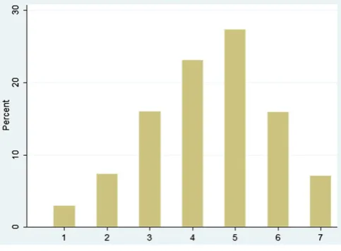
As our dependent variables we use data from the following two questions:‘How dissatisfied or satisfied are you with your life overall’

and‘How dissatisfied or satisfied are you with the amount of leisure time you have’. The respondents are asked to give a response on a 7-point scale, where the lowest value (1) is labelled‘Not Satisfied at all’and the highest value (7) is labelled‘Completely Satisfied’.6

Figs. 1 and 2present the distribution of the satisfaction with life overall and satisfaction with leisure time variables using data from all 12 waves available. It can be seen from the figure that the distribution of the overall life satisfaction data is highly skewed, with the majority of the responses at the top end of the distribution. This is a commonfinding in the literature on subjective well-being (Dolan et al., 2008). The distribution of the satisfaction with leisure time data is less skewed, but again the majority of the respondents report relatively high values.

As a robustness check, and to be consistent withRoberts et al. (2011), we also use the GHQ score as an alternative dependent variable in our analysis. The GHQ score is derived as the sum of the responses to 12 questions related to mental health each scored on a 4-point scale (from 0 to 3), where a high value represents a low level of mental health. In our analysis the score has been reversed so that a higher score represents better well-being. The distribution of the GHQ score using data from all 12 waves is shown inFig. 3.

The BHPS includes information on both commuting time and the mode of transport used for commuting trips.7_{The respondents are}

4

Baetschmann et al. (2011)also present Stata code for estimating the BUC model, but we have found that their code can inadvertently drop observations from the estimation sample in some circumstances. The root of the problem is that a new individual ID variable is generated by multiplying the original ID by 100 and adding a small number. Since the new ID variable is stored as a‘long’and the maximum value for longs is 2,147,483,620 in Stata, any individual with an original ID greater than 21,474,836 will drop out of the sample as their new ID will be set to‘missing’. This is an issue of practical importance using the original ID variable in the BHPS data–in our estimation sample a substantial propor-tion of respondents are incorrectly dropped when using the code by Baetschmann et al.

5

As expected the DvS estimator performs less well in situations where some cutoffs are associated with very small sample sizes.

6_{From wave 12 (2002) onwards the number 4 on the satisfaction scale was labelled} ‘Not satisfied/dissatisfied’, while it was unlabelled in earlier waves.Conti and Pudney (2011)find evidence that whether or not textual labels are assigned to values can have an impact on the results. As a robustness check we have therefore run the analysis in the paper on both the full (1996–2008) sample and the 2002–2008 sub-sample. As the re-sults are very similar we only report the full-sample analysis.

7_{The BHPS does not have data on commuting distance, but commuting time may in any}

asked‘How long does it usually take you to get to work each day, door to door?’. The answer is recorded in minutes and corresponds to a one-way commute. The respondents are then asked‘And what usually is your main means of travel to work?’. The response is coded as one of the following alternatives: car driver, car passenger, rail, underground, bus, motor bike, bicycle, walking and other.Fig. 4presents the distribu-tion of the commuting time variable using data from all 12 waves.

In addition to commuting time, which is the main explanatory vari-able of interest in our analysis, we control for a range of factors that have been found to be related to subjective well-being in previous work. These include age, hours worked, real household income (at 2008 prices), marital status, number of children in the household, a dummy for saving regularly and a dummy for having a university degree. As a sensitivity test we also interact commuting time with gender and muting mode to investigate whether the impact of an increase in com-muting time on well-being varies by gender and mode of transport.

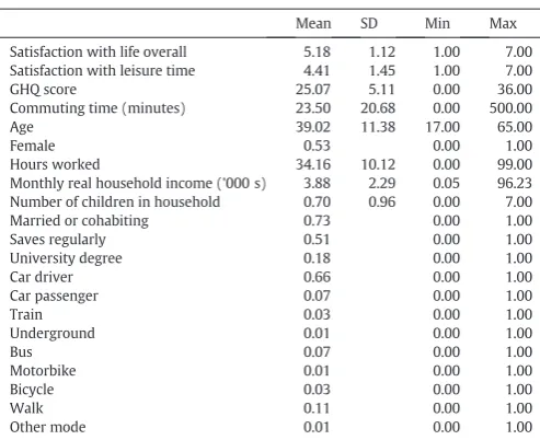
Table 1provides summary statistics for the estimation sample of the models with overall life satisfaction as the dependent variable.8_{It can be}

seen that the average daily commute is about 24 min (one way) and that most people drive a car to work. The average age in the sample is 39, about three quarters are married or cohabiting and the average number of children in the household is 0.7. About half of the sample make regular savings, 18% have a university degree and the average real monthly household income is £3900.

4. Results

4.1. Satisfaction with life overall

Table 2presents the results from the models of satisfaction with life overall.9 10 11_{It can be seen that while the coefficient for commuting}

time is negative and significant in the pooled ordered logit model (Pooled OL), it is insignificant in all thefixed-effects specifications. In line withBlanchflower and Oswald (2008)among others, wefind that satisfaction is U-shaped in age, with a minimum at around 54 years of age in the ordered FE specifications. Other significant variables include: (log) real household income (implying diminishing marginal utility of income), whether the respondent is married or cohabiting and whether he/she makes regular savings. These results are consistent with previ-ousfindings in the literature (Dolan et al., 2008; Wong et al., 2006).

The insignificant commuting time coefficient in the FE models con-trasts with thefindings byStutzer and Frey (2008)andRoberts et al. (2011)whofind that increases in commuting time are associated with lower levels of subjective well-being. Since Roberts et al. also use data from the BHPS but a different measure of subjective well-being (the GHQ score), we can test whether it is the choice of well-being measure that is driving the difference in the results. To do this we re-run our analysis using the GHQ score as the dependent variable instead of over-all life satisfaction.

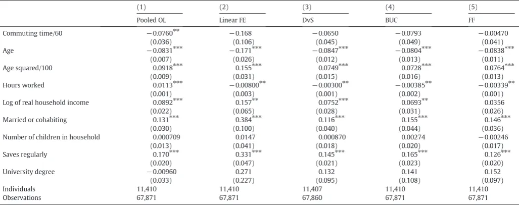
The results are reported inTable 3. Wefind no evidence of a negative relationship between commuting times and the GHQ measure of well-being in our sample, but when we re-run the analysis using data from waves 1–14 of the BHPS (the sample used by Roberts et. al) we are able to replicate their result that longer commuting times are associated with lower levels of well-being. We also_find that when we interact the commuting time variable with a dummy for being female this is found to be negative and significant in both samples, which supports Roberts et al.'sfinding that longer commutes are associated with lower levels of subjective well-being among women. We also attempted to include this interaction in the life satisfaction models, but it was found to be in-significant. This illustrates that different measures of subjective well-being may lead to different conclusions regarding policy relevant variables.

Stutzer and Frey (2008)use a very similar measure of well-being to ours, i.e. self-reported satisfaction with life overall. In this case the dif-ferentfindings may be due to cultural differences between the UK and Germany, although we concede that this is a somewhat speculative explanation.12_{What is clear, however, is that the}

‘commuting paradox_’ documented byStutzer and Frey (2008)does not hold in general, as we find no evidence of a negative impact of commuting times on life satis-faction in our application.

8

For the reasons discussed inSection 2the estimation sample does not include individ-uals who report constant life satisfaction scores over time, which leads to a decrease in the number of observations from 72,118 to 62,786. The characteristics of the two samples are very similar, however.

9

We‘Winsorise’the commuting time, hours worked and monthly household income data at the 99th centiles given the extreme upper values for these variables. Similar results to those presented in the paper are obtained if we simply trim the sample at the 99th centiles for these three variables, or Winsorise or trim at the 95th centile (results available on request).

10

We used 4, 5, 6 and 7 as the satisfaction cutoff-values in the DvS models as very few respondents report lower levels of life satisfaction than 4. This is the reason why the re-ported sample size for the DvS model is somewhat smaller than for the other models.

11_{For comparison we ran the pooled ordered logit and linearfixed-effects models on the}

same sample as the orderedfixed-effects models, i.e. excluding those respondents who re-ported the same level of satisfaction in all waves. Running the pooled ordered logit and lin-earfixed-effects models on the full sample gives very similar results.

12 _{One hypothesis we considered is that longer average commuting times may impact on}

social norms which in turn could potentially make the link between commuting times and well-being less strong. However, the average commuting time in our sample is only slight-ly higher than in the GSOEP sample used by Stutzer and Frey (24 vs 22 min) so this is un-likely to explain the differences in the results.

To test the robustness of the results we ran a further set of models where we interacted the commuting time variable with a set of dummies for commuting mode. None of these interactions were found to be significant. We also re-ran the models including the self-employed, adding a dummy for self-employment status to the models, but this was not found to have a qualitative impact on the results. The latter test was carried out to make our sample as similar as possible to that used byStutzer and Frey (2008), who included the self-employed in their analysis. Finally we tried controlling for part-time status and occupation in the models, but we do notfind evidence of a significant relationship between commuting and well-being for any of the occupa-tional groups. The results from the robustness checks are available from the authors upon request.

In line withFerrer-i-Carbonell and Frijters (2004)wefind that the results from the linear and ordered FE models are quite similar (in that the variables have the same signs and significance, the quadratic in age has a similar minimum point, etc.), considering the different assumptions underlying these models. Thisfinding contributes to the stock of evidence suggesting that a linear FE model is an acceptable sub-stitute for an ordered FE model in the context of modelling life satisfac-tion. However, this result needs to be tested on a case-by-case basis as there is no guarantee that it holds in general.

One advantage of the linear model over the ordered model is that the coefficients in the linear model can be interpreted as marginal ef-fects, while the coefficients in the ordered model cannot be interpreted

quantitatively since they refer to an underlying latent variable. In fact it is not possible to calculate marginal effects based on the FE ordered logit results at all since. However, as shown byFrey et al. (2009),Luechinger (2009), andLuechinger and Raschky (2009)for example, the ratios of the coefficients in the ordered model can be used to evaluate the trade-off between commuting time and income using the so-called

‘life satisfaction approach’.

To illustrate, letU=U(C,Y), whereCis commuting time andYis income. Totally differentiating and settingdU= 0 yields:

dY dC¼−

MUC

MUY

For our linearised specification with log income,U=βC+γlnY, this givesMUC=β,MUY=γ/Yand hence

dY dC¼−

βY γ

Evaluating this expression at median household incomeYMgives dY/dC=£1079 using the BUC estimates in Column 4 ofTable 2. Thus, at the median, commuters require compensation of £1000 of monthly household income per additional hour of (one-way) daily commuting time. This is equivalent to around £25 per hour of commuting time.13

Since the coefficient for commuting time is imprecisely estimated we cannot reject the null thatdY/dCis equal to zero14_{but this example}

nevertheless shows that the coefficients in the ordered FE models can be given a useful quantitative interpretation.

It is, of course, also possible to use the results from the linear FE model as a basis for calculating the increase in income necessary to compensate for an increase in commuting time. If we plug the estimated coefficients from the linear FE model into the expression fordY/dC

above we get £949, which is similar to thefigure derived from the BUC estimates. The question is then whether this is a coincidence or ev-idence of something more systematic. Based on a Monte Carlo study,

Riedl and Geishecker (2012)conclude the latter, and argue that the linear FE model is‘the method of choice’if the goal of the study is to estimate ratios of coefficients. To further examine this conclusion we have carried out a similar simulation study to that by Riedl and

13

Based on 20 days per month of commuting.

14

The lower and upper limit of a 95% CI calculated using the delta method are−£2570 and £4727, respectively.

Fig. 4.Distribution of daily commuting time (one way).

Fig. 3.Distribution of GHQ score.

Table 1

Summary statistics.

Mean SD Min Max Satisfaction with life overall 5.18 1.12 1.00 7.00 Satisfaction with leisure time 4.41 1.45 1.00 7.00 GHQ score 25.07 5.11 0.00 36.00 Commuting time (minutes) 23.50 20.68 0.00 500.00

Age 39.02 11.38 17.00 65.00

Female 0.53 0.00 1.00

Hours worked 34.16 10.12 0.00 99.00 Monthly real household income ('000 s) 3.88 2.29 0.05 96.23 Number of children in household 0.70 0.96 0.00 7.00 Married or cohabiting 0.73 0.00 1.00

Saves regularly 0.51 0.00 1.00

University degree 0.18 0.00 1.00

Car driver 0.66 0.00 1.00

Car passenger 0.07 0.00 1.00

Train 0.03 0.00 1.00

Underground 0.01 0.00 1.00

Bus 0.07 0.00 1.00

Motorbike 0.01 0.00 1.00

Bicycle 0.03 0.00 1.00

Walk 0.11 0.00 1.00

Geishecker (2012), where wefind that while the linear FE estimator does indeed do well in some settings, the BUC estimator clearly out-performs it in others. The simulations are described in detail in

Appendix A.

We therefore suggest that researchers implement ordered FE models when assessing the determinants of subjective well-being, rather than simply reporting the results from linear FE regressions which has become common in the literature. Treating well-being as an ordinal measure of individual welfare rather than assuming cardinal-ity as is required in the linear model is clearly preferred theoretically. And empirically, given the ease of implementation of the BUC and DvS estimators, plus the ability to interpret the ratio of coefficients in these specifications, means that an ordered approach can also yield interest-ing and interpretablefindings to the researcher.

4.2. Satisfaction with leisure time

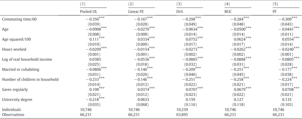
Table 4presents the results from the models of satisfaction with leisure time. In contrast to the life satisfaction results wefind that the coefficient for commuting time is negative and significant in all the specifications, suggesting that an increase in commuting time has a negative impact on the satisfaction with leisure time, as expected. Once again, there is evidence of a U-shaped relationship with age (with a minimum at around 40 years of age) and a positive relationship with making regular savings. Satisfaction with leisure time is found to be negatively related to hours worked, household income, the number of children in the household and being married or cohabiting. As in the life satisfaction case, the coefficients in the linear and ordered FE models generally have the same signs and significance.

Table 2

Satisfaction with life overall.

(1) (2) (3) (4) (5)

Pooled OL Linear FE DvS BUC FF

Commuting time/60 −0.237⁎⁎⁎ −0.0122 −0.0389 −0.0298 −0.0282

(0.039) (0.021) (0.049) (0.051) (0.045)

Age −0.104⁎⁎⁎ −0.0399⁎⁎⁎ −0.102⁎⁎⁎ −0.0958⁎⁎⁎ −0.108⁎⁎⁎

(0.008) (0.006) (0.014) (0.014) (0.012)

Age squared/100 0.121⁎⁎⁎ 0.0373⁎⁎⁎ 0.0933⁎⁎⁎ 0.0895⁎⁎⁎ 0.104⁎⁎⁎

(0.010) (0.007) (0.017) (0.018) (0.014)

Hours worked −0.00529⁎⁎⁎ −0.000744 −0.00267 −0.00162 −0.00140

(0.001) (0.001) (0.002) (0.002) (0.002)

Log of real household income 0.197⁎⁎⁎ 0.0448⁎⁎⁎ 0.0995⁎⁎⁎ 0.0962⁎⁎⁎ 0.0852⁎⁎⁎

(0.026) (0.014) (0.031) (0.032) (0.029)

Married or cohabiting 0.589⁎⁎⁎ 0.206⁎⁎⁎ 0.464⁎⁎⁎ 0.466⁎⁎⁎ 0.403⁎⁎⁎

(0.032) (0.021) (0.047) (0.049) (0.040)

Number of children in household −0.0509⁎⁎⁎ −0.00936 −0.0348⁎ −0.0303 −0.0207

(0.015) (0.009) (0.021) (0.021) (0.018)

Saves regularly 0.299⁎⁎⁎ 0.0886⁎⁎⁎ 0.212⁎⁎⁎ 0.216⁎⁎⁎ 0.200⁎⁎⁎

(0.022) (0.010) (0.023) (0.024) (0.023)

University degree −0.0219 0.0530 0.0975 0.126 0.175

(0.035) (0.052) (0.123) (0.128) (0.109)

Individuals 9930 9930 9863 9930 9930

Observations 62,786 62,786 62,537 62,786 62,786

Standard errors in parentheses.

⁎pb0.10,⁎⁎pb0.05,⁎⁎⁎pb0.01.

Table 3

GHQ score.

(1) (2) (3) (4) (5)

Pooled OL Linear FE DvS BUC FF

Commuting time/60 −0.0760⁎⁎ −0.168 −0.0650 −0.0793 −0.00470

(0.036) (0.106) (0.045) (0.049) (0.041)

Age −0.0831⁎⁎⁎ −0.171⁎⁎⁎ −0.0847⁎⁎⁎ −0.0804⁎⁎⁎ −0.0838⁎⁎⁎

(0.007) (0.026) (0.012) (0.013) (0.011)

Age squared/100 0.0918⁎⁎⁎ 0.155⁎⁎⁎ 0.0749⁎⁎⁎ 0.0728⁎⁎⁎ 0.0764⁎⁎⁎

(0.009) (0.031) (0.015) (0.016) (0.013)

Hours worked 0.0113⁎⁎⁎ −0.00800⁎⁎ −0.00300⁎⁎ −0.00385⁎⁎ −0.00339⁎⁎

(0.001) (0.003) (0.001) (0.002) (0.001)

Log of real household income 0.0892⁎⁎⁎ 0.157⁎⁎ 0.0752⁎⁎⁎ 0.0693⁎⁎ 0.0356

(0.022) (0.065) (0.028) (0.031) (0.026)

Married or cohabiting 0.131⁎⁎⁎ 0.384⁎⁎⁎ 0.116⁎⁎⁎ 0.155⁎⁎⁎ 0.146⁎⁎⁎

(0.030) (0.100) (0.040) (0.044) (0.036)

Number of children in household 0.000709 0.0147 0.000870 0.00274 −0.00246

(0.013) (0.041) (0.018) (0.020) (0.017)

Saves regularly 0.170⁎⁎⁎ 0.331⁎⁎⁎ 0.145⁎⁎⁎ 0.165⁎⁎⁎ 0.126⁎⁎⁎

(0.020) (0.047) (0.021) (0.023) (0.020)

University degree −0.00960 0.271 0.132 0.141 0.152

(0.033) (0.227) (0.095) (0.108) (0.097)

Individuals 11,410 11,410 11,407 11,410 11,410

Observations 67,871 67,871 67,860 67,871 67,871

Standard errors in parentheses.

5. Conclusion

This paper provides an assessment of alternative estimators for the fixed-effects ordered logit model in the context of estimating the rela-tionship between subjective well-being and commuting behaviour. In contrast toStutzer and Frey (2008)wefind no evidence that longer commutes are associated with lower levels of subjective well-being as measured by self-reported overall life satisfaction. When using the GHQ score as an alternative measure of subjective well-being wefind, in line withRoberts et al. (2011), that longer commutes are associated with lower levels of well-being for women but not for men. Taken as a whole thesefindings suggest that the‘commuting paradox’ document-ed byStutzer and Frey (2008)does not hold in general.

While our empirical results support earlierfindings in the literature that linear and ordered_fixed-effects models of life satisfaction give sim-ilar results, we argue that ordered models are more appropriate since they do not require the researcher to make the questionable assumption that life satisfaction scores are cardinal. We also demonstrate that the ordered models are straightforward to implement in practice and lead to readily interpretable results. We therefore recommend that ordered fixed effects models are used to model life satisfaction instead of linear models, as the latter rely on an empirical regularity that may not always hold. This conclusion is supported by a simulation study which demon-strates that the BUC estimator clearly outperforms the linear FE estima-tor in some settings.

Finally, we have demonstrated how models of well-being can be used to provide an alternative approach to estimating the marginal will-ingness to pay for commuting, in contrast to standard hedonic wage re-gressions and other approaches (see, for example,Van Ommeren et al. (2000)).

Appendix A. Simulations

In this Appendix we investigate using simulated data whether the linearfixed-effects (FE) estimator produces unbiased estimates of coef-ficient ratios when the true model is an FE ordered logit. As described below wefind that the linear FE estimator does well in some settings, while the BUC estimator clearly outperforms it in others.

A.1. Data Generation Process (DGP) 1

The true model is

yit¼β1xit1þβ2xit2þαiþεit; i¼1;…;1000 t¼1;…;10

where

β1= 1,β2= 0.5, αi~N(0, 0.5)

xit1¼αiþvit; vitNð0;0:5Þ

xit2~N(0, 1) εit~Logistic(0, 1)

This implies that the marginal distributions ofxit1andxit2are both

standard normal, and the correlation betweenxit1andαiis about 0.7.

The dependent variableyitis generated according to the following rule

yit¼k if μkbyit≤μkþ1; k¼1;…;7

where the values of the threshold parameters,μk, are set to mimic the distribution of the life satisfaction variable in the BHPS. We generate 10,000 datasets with 10 observations on 1000‘individuals’, and for each of these datasets we estimate the coef_ficients in the model using three different estimators: pooled ordered logit, linear FE and BUC. The mean of the estimated coefficient ratio and the root-mean-square error (RMSE) of the estimate are reported in the table below:

Table A1

Simulation results—DGP1. (1) Pooled OL

(2) Linear FE

(3) BUC

Mean of^β1=β^2 3.004 2.004 2.004

RMSE 1.012 0.104 0.105

It can be seen from the table that the pooled OL estimator is biased, which is to be expected given the correlation betweenxit1and the

indi-vidual effectαi. The linear FE and BUC estimators are both effectively

Table 4

Satisfaction with leisure time.

(1) (2) (3) (4) (5)

Pooled OL Linear FE DvS BUC FF

Commuting time/60 −0.350⁎⁎⁎ −0.167⁎⁎⁎ −0.298⁎⁎⁎ −0.284⁎⁎⁎ −0.309⁎⁎⁎

(0.039) (0.028) (0.049) (0.048) (0.043)

Age −0.0908⁎⁎⁎ −0.0270⁎⁎⁎ −0.0634⁎⁎⁎ −0.0500⁎⁎⁎ −0.0441⁎⁎⁎

(0.008) (0.008) (0.014) (0.014) (0.011)

Age squared/100 0.111⁎⁎⁎ 0.0334⁎⁎⁎ 0.0752⁎⁎⁎ 0.0624⁎⁎⁎ 0.0554⁎⁎⁎

(0.010) (0.009) (0.017) (0.017) (0.014)

Hours worked −0.0209⁎⁎⁎ −0.0154⁎⁎⁎ −0.0273⁎⁎⁎ −0.0262⁎⁎⁎ −0.0240⁎⁎⁎

(0.001) (0.001) (0.002) (0.002) (0.001)

Log of real household income 0.0385 −0.0536⁎⁎⁎ −0.0885⁎⁎⁎ −0.0888⁎⁎⁎ −0.0805⁎⁎⁎

(0.025) (0.018) (0.032) (0.031) (0.028)

Married or cohabiting −0.0806⁎⁎⁎ −0.146⁎⁎⁎ −0.209⁎⁎⁎ −0.251⁎⁎⁎ −0.177⁎⁎⁎

(0.031) (0.026) (0.046) (0.045) (0.038)

Number of children in household −0.233⁎⁎⁎ −0.146⁎⁎⁎ −0.251⁎⁎⁎ −0.258⁎⁎⁎ −0.224⁎⁎⁎

(0.014) (0.012) (0.022) (0.021) (0.017)

Saves regularly 0.198⁎⁎⁎ 0.0374⁎⁎⁎ 0.0707⁎⁎⁎ 0.0679⁎⁎⁎ 0.0708⁎⁎⁎

(0.021) (0.012) (0.023) (0.022) (0.021)

University degree −0.218⁎⁎⁎ 0.0633 0.159 0.127 0.135

(0.035) (0.068) (0.116) (0.118) (0.103)

Individuals 10,746 10,746 10,239 10,746 10,746

Observations 66,231 66,231 63,895 66,231 66,231

Standard errors in parentheses.

unbiased, and the RMSE of the linear FE estimator is similar to that of the BUC estimator (in fact it is slightly lower). This confirms thefinding in

Riedl and Geishecker (2012)that linear FE models can give unbiased re-sults of coefficient ratios when the dependent variable is ordinal. As we will see in the following section, however, this result does not hold in general.

A.2. DGP 2

The true model is

yit¼β1Dit1þβ2Dit2þαiþεit; i¼1;…;1000 t¼1;…;10

where

β1= 1,β2= 0.5,

Dit1= 1 ifxit1N1 and 0 otherwise

Dit2= 1 ifxit2N1 and 0 otherwise

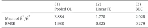
The remaining variables are defined as before and the values of the threshold parameters,μk, are set to mimic the distribution of the life sat-isfaction variable in the BHPS. The key difference between DGP1 and DGP2, therefore, is that the two regressors are now dummy variables, which take the value 1 for about 16% of the observations. The results, based on 10,000 replications, are reported in the table below.

Table A2

Simulation results—DGP2. (1) Pooled OL

(2) Linear FE

(3) BUC

Mean of^β1=β^2 3.884 1.778 2.026

RMSE 1.938 0.325 0.279

In this case it is clear that the BUC estimator outperforms the linear FE estimator: the mean of the BUC coefficient ratio is closer to the true value and its RMSE is lower than that of the linear estimator. These re-sults demonstrate that the linear FE estimator is not an equally good op-tion for estimating coefficient ratios in all cases.

A.3. DGP 3

From the above it may be tempting to conclude that the linear FE es-timator does as well as the BUC eses-timator as long as the explanatory var-iables are continuous. However, we will see that that is not the case; it is possible for the linear FE estimator to do less well than the BUC estima-tor also when the regressors have continuous distributions. To illustrate we will use an example in which the regressors are both discrete mix-tures of two log-normally distributed variables. The particular choice of distribution is not important, however; our aim is simply to demon-strate that the BUC estimator can outperform the linear FE estimator when the regressors are continuous.

The true model is

yit¼β1zit1þβ2zit2þαiþεit; i¼1;…;1000 t¼1;…;10

where

β1= 1,β2= 0.5,

zit1=Dit1uit1+ (1−Dit1)uit2

zit2=Dit2uit1+ (1−Dit2)uit2

ln(uit1) ~N(−0.5, 0.5)

ln(uit2) ~N(0.5, 0.5)

The remaining variables are defined as before and the values of the threshold parameters,μk, are set to mimic the distribution of the life

satisfaction variable in the BHPS. The results, based on 10,000 replica-tions, are reported in the table below.

Table A3

Simulation results—DGP3. (1) Pooled OL

(2) Linear FE

(3) BUC

Mean of^β1=β^2 1.705 1.907 2.008

RMSE 0.316 0.154 0.139

Again we can see that the BUC estimator does better than the linear FE estimator. While it could be argued that the performance of the linear FE estimator is notmuchworse than BUC, we cannot know whether that will always be the case; other data generation processes may lead to larger differences in performance. The fact that we have evidence that the linear FE estimator can in some cases perform less well suggests that it is prudent to err on the side of caution and use the BUC estimator instead. The argument for this strategy is made more compelling by the fact that the BUC estimator is straightforward to implement and leads to easily interpretable results, as we demonstrate in this paper.

Appendix B. Stata code

B.2. BUC code

References

Abrantes, P.A.L., Wardman, M.R., 2011.Meta-analysis of UK values of travel time: an update. Transp. Res. A 45, 1–17.

Baetschmann, G., Staub, K.E., Winkelmann, R., 2011.Consistent estimation of thefixed effects ordered logit model. IZA Discussion Paper #5443.

Blanchflower, D.G., Oswald, A.J., 2008.Is well-being U-shaped over the life cycle? Soc. Sci. Med. 66 (8), 1733–1749.

Booth, A., Van Ours, J., 2008.Job satisfaction and family happiness: the part-time work puzzle. Econ. J. 118, F77–F99.

Booth, A., Van Ours, J., 2009.Hours of work and gender identity: does part-time work make the family happier? Economica 76, 176–196.

Chamberlain, G., 1980.Analysis of covariance with qualitative data. Rev. Econ. Stud. 47 (1), 225–238.

Clark, A., Frijters, P., Shields, M., 2008.Relative income, happiness and utility: an explanation for the Easterlin paradox and other puzzles. J. Econ. Lit. 46 (1), 95–144.

Conti, G., Pudney, S., 2011.Survey design and the analysis of satisfaction. Rev. Econ. Stat. 93 (3), 1087–1093.

Das, M., Van Soest, A., 1999.A panel data model for subjective information on household income growth. J. Econ. Behav. Organ. 40 (4), 409–426.

Di Tella, R., MacCulloch, R., 2006.Some uses of happiness data in economics. J. Econ. Perspect. 20 (1), 25–46.

Dolan, P., Peasgood, T., White, M., 2008.Do we really know what makes us happy? A re-view of the economic literature on the factors associated with subjective well-being. J. Econ. Psychol. 29 (1), 94–122.

Ferrer-i-Carbonell, A., Frijters, P., 2004.How important is methodology for the estimates of the determinants of happiness? Econ. J. 114 (497), 641–659.

Frey, B.S., Stutzer, A., 2000.Happiness, economy and institutions. Econ. J. 110 (466), 918–938.

Frey, B.S., Stutzer, A., 2002a.Happiness and Economics: How the Economy and Institu-tions Affect Well-being. Princeton University Press, Princeton and Oxford.

Frey, B.S., Stutzer, A., 2002b.What can economists learn from happiness research? J. Econ. Lit. 40 (2), 402–435.

Frey, B.S., Luechinger, S., Stutzer, A., 2009.The life satisfaction approach to environmental valuation. IZA Discussion Paper #4478.

Greene, W., 2004.The behaviour of the maximum likelihood estimator of limited dependent variable models in the presence offixed effects. Econ. J. 7 (1), 98–119.

Jones, A., Schurer, S., 2011.How does heterogeneity shape the socioeconomic gradient in health satisfaction? J. Appl. Econ. 26 (4), 549–579.

Kahneman, D., Krueger, A.B., 2006.Developments in the measurement of subjective well-being. J. Econ. Perspect. 20 (1), 3–24.

Kassenboehmer, S., Haisken-DeNew, J., 2009.You'refired! The causal negative effect of entry unemployment on life satisfaction. Econ. J. 119, 448–462.

Layard, R., 2005.Happiness: Lessons from a New Science. Penguin, New York.

Luechinger, S., 2009.Valuing air quality using the life satisfaction approach. Econ. J. 119 (536), 482–515.

Luechinger, S., Raschky, P.A., 2009.Valuingflood disasters using the life satisfaction approach. J. Public Econ. 93 (3–4), 620–633.

MacKerron, G., 2012.Happiness economics from 35,000 feet. J. Econ. Surv. 26 (4), 705–735.

Mundlak, Y., 1978.On the pooling of time-series and cross-section data. Econometrica 46, 69–85.

Neyman, J., Scott, E., 1948.Consistent estimates based on partially consistent observations. Econometrica 16 (1), 1–32.

Pierrard, O., 2008.Commuters, residents and job competition. Reg. Sci. Urban Econ. 38 (6), 565–577.

Riedl, M., Geishecker, I., 2012.Keep it simple: estimation strategies for ordered response models withfixed effects. Working Paper, Faculty of Economic Sciences, Georg-August-Universität Göttingen.

Roberts, J., Hodgson, R., Dolan, P., 2011.‘It's driving her mad’: gender differences in the effects of commuting on psychological health. J. Health Econ. 30 (5), 1064–1076.

Ross, S.L., Zenou, Y., 2008.Are shirking and leisure substitutable? An empirical test of efficiency wages based on urban economic theory. Reg. Sci. Urban Econ. 38 (5), 498–517.

Stutzer, A., Frey, B.S., 2008.Stress that doesn't pay: the commuting paradox. Scand. J. Econ. 110 (2), 339–366.

Stutzer, A., Frey, B.S., 2010.Recent advances in the economics of individual subjective well-being. Soc. Res. 77 (2), 679–714.

van Ommeren, J.N., Gutiérrez-i-Puigarnau, E., 2011.Are workers with a long commute less productive? An empirical analysis of absenteeism. Reg. Sci. Urban Econ. 41 (1), 1–8.

Van Ommeren, J., van den Berg, G., Gorter, C., 2000.Estimating the marginal willingness to pay for commuting. J. Reg. Sci. 40 (3), 541–563.

Winkelmann, L., Winkelmann, R., 1998.Why are the unemployed so unhappy? Evidence from panel data. Economica 65 (257), 1–15.