
Trace elements in coal from Colinsville, Bowen basin, Australia : in-ground mode of occurrence and behaviour during utilisation
532
0
0
Full text
(2)
(3)
(4)
(5) ii Abstract.. Analysis of samples gathered during delineation of a coal resource is becoming increasingly sophisticated as various organisations attempt to predict and understand the technological behaviour of the mined product. Analysis to determine the concentration of trace elements in coal is becoming more prevalent, and not just merely for academic curiosity. Increased environmental awareness has impelled the need to consider potential negative impacts on the ecosystem caused by liberation of trace elements from coal during utilisation.. The aims of this thesis are to: 1) Determine the concentration of trace elements in coal seams mined to supply the Collinsville pulverised fuel combustion plant at the Collinsville open cut, Northern Bowen Basin, Australia; 2) Determine the mineralogy and, using graphical relationships, the likely mode of occurrence of trace elements in the sampled pits; 3) Determine the mode of occurrence of trace elements in the pulverised fuel of the Collinsville power plant using the USGS sequential leaching method, and contrast the results with the same analysis for an unrelated fuel from another coal fired power utility (Mitsui Mining’s Omutu City plant, Kyushu, Japan); 4) Examine the partitioning behaviour of trace elements in the Collinsville power utility, and contrast the results with the partitioning behaviour of trace elements in the Mitsui combustion utility to assess the influence of trace element mode of occurrence on partitioning behaviour; 5) Examine the mobility of trace elements from solid ash waste from the Collinsville power utility, and compare with the mobility of trace elements from the Mitsui power utility solid waste to assess the influence of mode of occurrence on the leachability of trace elements and; 6) Determine the partitioning behaviour of trace elements in carbonisation of Bowen seam coal at the Bowen coke works and compare with the partitioning behaviour of the same elements in combustion.. Lithotype logging of coal exposed in the highwalls of the Blake Central, Blake West and Bowen No.2 pits was undertaken. Of particular note was the presence of dull heat affected coal toward the roof of the Blake Central pit seam, toward the floor of the.
(6) iii Bowen No.2 pit seam, and the presence of bed-parallel intrusions within the seam in the Blake West pit. In the Blake West pit seam, the intrusion caused thermal alteration of the coal to coke over a 60cm zone immediately adjacent to the intrusion with a further 1.101.25m zone of dull heat altered coal beyond the coked zone. In the Blake Central, 4.5m of dull heat-affected coal occurred near the roof of the seam. In the Bowen No.2 pit, 1.2m of heat-affected coal occurred near the floor of the seam. Beyond the heat affected zone, lithotype logging of the Blake seams noted a number of rock partings, but no convincing dulling upward cycles due to progressive drying of the mire, noted in other studies of Permian coal, were found. No partings were found in the Bowen seam and only one convincing dulling upward cycles was logged. In part the absence of dulling upward cycles is due to heat alteration of the coal, but the numerous influxes of sediment laden water into the Blake seam mire also acted to terminate any significant dulling upward cycles by raising both nutrient levels and the water table.. Following lithotype logging, channel sampling of the pits resulted in a total of 76 samples, 25 from the Blake Central pit, 36 from the Blake West pit and 15 from the Bowen No.2 pit. The channel sampling intervals were determined approximately by coal lithotype interval, with some amalgamations to restrict sample numbers. The channel samples were analysed for proximate analysis, coal petrography and vitrinite reflectance (selected samples) and for major and trace elements using XRF and INAA.. The lithotype logs, proximate analysis data and coal petrography were integrated to infer the depositional environment of the Blake and Bowen seams. The generally high ash yield, common stone bands, low sulphur content of the coal and rare pyrite in the Blake seam suggests the depositional environment was a Class 3 topotelmitic peat with a variable water table. The moderate ash yield, the absence of common stone bands, sulphur contents of ~2% and the moderate pyrite content of the coal in the Bowen seam suggests the depositional environment was a Class 2 topotelmitic peat with a high water table..
(7) iv The igneous intrusions have caused extensive alteration of vitrinite to semi-coke, a general decrease in the volatile matter content and an increase in the vitrinite reflectance [Ro(max)] toward the intrusion.. Mineralogy was calculated from major and trace elements using normative analysis, calibrated by XRD analysis of low temperature ash from selected samples. The mineralogy of the Blake seam samples is dominated by kaolinite, with subordinate quartz, illite, feldspar, and siderite, and minor concentrations of pyrite, gorceixite, goyazite and anatase. The mineralogy of the Bowen seam samples is dominated by kaolinite, with subordinate quartz, illite and pyrite, and minor concentrations of siderite, gorceixite, goyazite and anatase/ rutile/ iron oxides.. The concentration of trace elements in the channel samples was determined by INAA and XRF. The INAA and XRF concentrations of iron and uranium show a reasonable statistical relationship suggesting the two analysis methods are consistent with each other. The concentration of trace elements in the Blake and Bowen seams is generally low compared to world average ranges for coal and to crustal averages. Only gold, copper, hafnium, thorium and ytterbium were found to be above the world coal average range in the Blake seam. Only gold and copper were found to be above world coal average range in the Bowen seam coal.. Trace element mode of occurrence was inferred using graphical relationships between normative mineral and trace element concentrations. In the Blake seam, arsenic, possibly chromium, copper, mercury, nickel and lead were inferred to be associated with pyrite. Bromine, cobalt, selenium, and zinc appeared to be organically bound. Cerium, caesium, europium, lanthanum, rubidium, and scandium showed a graphical relationship with illite. However, cerium, europium, lanthanum and scandium, along with hafnium, lutetium, neodymium, samarium, terbium, thorium, uranium and vanadium also showed a graphical relationship with gorceixite or gorceixite plus goyazite. It was inferred the latter group of elements are associated with monazite or zircon. In addition to the REE phosphate mode of occurrence, some rare earth elements also showed an affinity for.
(8) v kaolinite. Thorium and uranium were also inferred to be associated with feldspars. Antimony, tantalum and ytterbium were found to be dominantly associated with kaolinite.. In the Bowen seam, arsenic, cobalt, possibly chromium, copper, mercury, molybdenum, nickel, lead, antimony, selenium and zinc showed a graphical relationship with pyrite. The elements cerium, hafnium, neodymium, rubidium, samarium, tantalum, thorium, uranium and tungsten all showed significant graphical relationships with the anatase/ rutile/ FeO grouping of minerals. It is inferred that the relationship is due to the presence of monazite, zircon, xenotime, REE phosphates, tungstates or other trace minerals, the distribution of which mirrors the distribution of the anatase/ rutile/ FeO grouping. Uranium and thorium were inferred to be associated with REE phosphates and zircon respectively, plus illite. The elements bromine, europium, lanthanum, terbium and vanadium were inferred to be associated with illite. A mixed illite/ heavy mineral suite mode of occurrence is inferred for samarium, tantalum, thorium and uranium. The elements caesium, lutetium, scandium, and ytterbium were inferred to be associated with kaolinite.. The effect of igneous intrusions on the concentration of a number of minerals and trace elements was also examined. The presence of semi-coke or an inferred distance of heat alteration was used to distinguish heat affected and unaffected samples. Depletion or enrichment of minerals and elements was inferred using ply thickness weighted average concentration figures for altered and unaltered samples and trends of concentration change toward the intrusion. Some consistent changes in the concentration of trace elements and minerals were found across all three pits sampled. The minerals siderite and pyrite are depleted in the heat affected zone, but goyazite is enriched, particularly toward the margins of the heat affected zone. The elements bromine and strontium (the latter mirroring the goyazite trend) are concentrated in the heat affected zone. The elements cobalt, mercury, manganese (mirroring the pyrite trend), nickel and possibly arsenic and zinc are depleted in heat affected samples from all three pits sampled. The inconsistent behaviour of some other trace elements (molybdenum, chromium and.
(9) vi possibly selenium) in response to the igneous intrusion appears to be the result of different modes of occurrence of trace elements between pits.. Samples of pulverised fuel were collected from the Collinsville and Japanese (Mitsui) pulverised fuel utilities. The concentration of major and trace elements was determined by INAA, XRF and (for the Collinsville sample) ICP-MS & ICP-AES. INAA analysis suggests gold, cerium, cobalt, europium, hafnium, lanthanum, lutetium, molybdenum, neodymium, scandium, selenium, samarium, strontium, tantalum, thorium, tungsten and ytterbium are at the upper end or above the world average concentration range in the Collinsville pulverized fuel. Only gold, hafnium and thorium are at the upper end or above the world coal concentration range in the Japanese pulverized fuel.. Sequential leaching of the pulverised fuels was undertaken according to the USGS protocol. The sequential leach data was interpreted to infer trace element mode of occurrence in the pulverised fuel. A number of significant differences in the mode of occurrence of antimony, arsenic, chromium, cobalt, nickel, selenium, uranium and zinc were found between the two combustion plants studied. The element vanadium had almost identical modes of occurrence in fuel from both plants studied.. A comparison of trace element mode of occurrence determined for the Collinsville power utility pulverised fuel by sequential leaching with mode of occurrence determined for the in-ground feed coals using graphical methods showed a reasonable level of agreement. It is concluded that the use of two methods of determining mode of occurrence provides better definition of mineral type in some cases. For example a siderite mode of occurrence could be determined using graphical relationship whereas the sequential leach data gave only a carbonate mode of occurrence. Further, the sequential leach data solved the problem of parallel graphical relationships. For example, galena was determined to be the mode of occurrence of lead from the sequential leach data, whereas graphical relationships indicated a pyrite mode of occurrence because of the relationship with sulphur..
(10) vii Combustion of coal occurs in three phases, namely devolatilisation, combustion of the volatile matter, and combustion of the residual char. Mineral matter may be excluded from the residual char particles due to desegregation and separation in the milling process, or included within the char particle. During combustion, trace elements partition between the bottom ash, the fly ash, and flue gas (lost up the stack). The concentration of trace elements in ash samples from the Collinsville and Mitsui power utilities was determined by INAA and XRF. The partitioning behaviour of the trace elements is examined by calculating relative enrichment values for the trace elements. Generally the partitioning behaviour and classification of trace elements in this study matched those found in previous published studies for a given element.. The relative enrichment trends of elements exhibiting significant differences in mode of occurrence between the two combustion plants sampled (ie antimony, arsenic, chromium, cobalt, nickel, selenium, uranium and zinc plus vanadium) were examined to determine the control of mode of occurrence on the partitioning behaviour. It is hypothesised that the relative volatility of a particular element in combustion reflects the temperature at which the host mineral or the organic matter thermally decomposes. Thus organically bound elements should be more volatile than pyrite associated elements, which should be more volatile than carbonate associated elements, which should be substantially more volatile than silicate associated elements. Other factors that may influence partitioning behaviour such as the major element chemistry of the ash, plant design and operating conditions, and temperature variations within the combustion chamber were discounted as significantly influencing relative enrichment differences for the two combustion plants studied. It is concluded that element mode of occurrence has a strong influence on the relative volatility of a given element, and that comparison of sequential leach results from two pulverised fuel utilities has the potential allow prediction of the relative volatility of trace elements in combustion. Some complications may arise due to exclusion of some mineral grains and localised variations in the oxidation state within the combustion zone.. Solid combustion wastes (fly ash and bottom ash) are commonly disposed of in landfill and impoundment facilities. Unless the landfill is impermeable to water, disposal of solid.
(11) viii wastes in such fashion allows interaction with the hydrogeological system and could lead to detrimental environmental impacts. Leaching of indicative “total waste” composites made up by blending fly ash and bottom ash samples from each power utility in an 80/20 proportion was undertaken using the TCLP protocol. The concentration of trace elements in the leachates was compared to recreational water and drinkwater guideline values. The concentration of barium, manganese, and selenium in the Collinsville leachate exceeds both the recreational and drinkwater guideline concentrations. The concentration of nickel in the Collinsville leachate was found to exceed the recommended drinkwater concentration, but is below recreational water guideline value. The concentration of boron and selenium in the Mitsui leachate was found to exceed both the recreational and drinkwater guideline values. The concentration of barium in the Mitsui leachate was found to exceed the drinkwater standard. The concentration of an element in the ash sample was found to be a poor indicator of the mobility of the element.. Elements that showed substantial differences in mode of occurrence in the pulverised fuel (ie antimony, arsenic, chromium, cobalt, nickel, selenium, uranium and zinc plus vanadium) were examined to assess the influence of mode of occurrence on the leachability of the element from solid combustion waste. It is concluded that, where the difference in element mobility between the two composite ash samples is significant, mode of occurrence does exert some control on the proportion of a trace element in the ash that can be mobilised by the TCLP protocol. In particular, trace elements present in coal associated with silicates appear substantially unavailable for mobilisation by the TCLP protocol.. The concentration of trace elements in samples of feed coal, coke and breeze from the Bowen coke works was determined by INAA and XRF. A new index (the CRE index) was developed to characterise the enrichment or depletion of trace elements in the coke and breeze. Coke is classified as enriched (Class 1), neither enriched nor depleted (Class 2), depleted (Class 3) or highly depleted (Class 4). Breeze was classified as enriched (denoted “e”), neither enriched nor depleted (denoted “a”) and depleted (denoted “d”)..
(12) ix Comparison of the partitioning behaviour of trace elements in combustion and carbonisation was undertaken by comparing the RE and CRE data. It is concluded that all but the most volatile elements (sulphur, selenium, arsenic and tungsten) are substantially retained in the coke. The substantial retention of trace elements in coke is likely due to the lower temperature at which carbonisation occurs compared to pulverised fuel combustion temperatures. The behaviour of trace elements in the breeze is similar to their behaviour in combustion, being controlled by mode of occurrence end element volatility. Trace elements associated with pyrite are generally enriched in the breeze, excepting highly volatile elements such as sulphur, selenium and arsenic, which appear to substantially volatilise. Silicate associated elements and those elements associated with heavy minerals are also generally non-volatile excepting tungsten that is depleted in the coke and breeze.. The concentration of trace elements in the pit channel samples and in the pulverised fuel sample suggest the elements barium, selenium, mercury, thorium, copper, manganese, nickel and vanadium warrant further investigation in Collinsville pit and combustion wastes. The data suggests the elements thorium, boron, selenium and barium warrant further investigation in the Japanese combustion plant. Further work to verify that relative differences in mode of occurrence inferred from USGS sequential leaching are useful as indicators of trace element volatility and leachability is recommended.. The environmentally significant trace elements cobalt, molybdenum, antimony, strontium, zinc and possibly arsenic and chromium are enriched in the breeze samples from the Bowen coke works. Leaching studies to determine the proportion and concentration of trace elements in the leachate upon disposal of the waste is worth consideration. Further studies to characterise trace element partitioning during carbonisation in a slot oven are recommended..
(13) x Acknowledgements.. I would like to thank the following people for their assistance with this PhD. My supervisor Dr Peter Crosdale, who organised research grants and a scholarship at James Cook University, provided accommodation to the entire family for our first two weeks in Townsville, provided training in the petrography of Australian coals, introduced me to all the right people (and a few of the wrong ones at wine club) and then watched bemused as we all moved back to New Zealand ten months later to resume full time employment. Dr Crosdale also undertook a thorough and useful review of manuscript drafts. Thank you for your technical advice, encouragement and forbearance. I did eventually finish the thesis! Mr Ray Slater (then Resource Management Superintendent at the Collinsville coal mine) for his considerable help and advice, the benefit of his expertise on the Collinsville operations, organising access to the mine to undertake sampling, and organising the saving of splits of the Bowen coke works train samples. Thank you also to Theiss mining contractors, Collinsville for covering the cost of the proximate analysis of the pit channel samples. Mr Ian Borthwick for providing access to the Collinsville power utility and gathering samples of pulverised fuel, bottom ash and fly ashes. Mr Oki Nishioka for organising the gathering of coal and ash samples at Mitsui Mining’s Omutu City pulverised coal combustion utility in Kyushu, Japan. Mr John Laidlaw for allowing access to the Bowen coke works and for gathering samples of coke and breeze over several months. Messrs Hugh McMillan and Trevor Daly of SGS Ngakawau, New Zealand for undertaking low temperature ashing and sulphur analysis of numerous samples. Dr Jane Newman for agreeing to train me (once again!) in the measurement of vitrinite reflectance and coal petrography point counting. Also for the encouragement that a PhD could be completed part time and some inspirational discussions on coal science over a lot of years. Mr Colin Nunweek is thanked for mounting the petrographic samples under Dr Newman’s supervision. Thanks to the Geology Department, University of Canterbury, New Zealand for providing access to use the petrographic microscope. Particular thanks to Dr Kerry Swanson, who always seemed to have an appropriate sized “bit of wire” to carry out the odd technical fix..
(14) xi Dr Nigel Newman of CRL Energy for undertaking low temperature ashing and organising XRD analysis of selected samples, and for some useful observations on the results. Thanks to the United States Geological Survey, particularly Dr Bob Finkelman and Dr Curtis Palmer for undertaking sequential leaching analysis of the Collinsville pulverised fuel as part of the world Coal Quality Database programme; also for supplying a number of useful papers and some helpful correspondence. Also particular thanks to Dr Palmer who assisted with the preparation and explanation of the chondrite normalised plots. Dr Zhongsheng Li, for setting up and running the sequential leaching of the Japanese pulverised fuel sample at Canterbury University, Christchurch, New Zealand. Particular thanks to Solid Energy New Zealand, especially Mr Barry Bragg, for organising substantial funding to cover the XRF analytical costs over the latter stages of this project and providing an extra week of leave a year for the past three years. Thanks to Dr Doug Lewis who inspired a enthusiasm for research and technical reading, and Mr Frank Taylor who gave me my first coal job and instilled a sense of the value of practical geology. Thanks also to my “room mate” at Solid Energy Jonny McNee for the laughs. My parents, David and Anne, who taught me the value working to achieve a goal, and have continuing to be there for advice, encouragement and the occasional meal and accommodation for studies in Christchurch. And finally to my wife Fran, who packed up the household to move to Australia so I could quit work and go back to uni, and then packed it up to move back again so I could go back to work and study as well!!; who watched family finances disappear into the analytical bills black hole and assorted text books; who understood when I disappeared night after night into the study and worked at weekends instead of doing the garden; who listened to my inane ravings, and who remained lovingly supportive. Also to my children Erica and Michelle, who have had to be content with short hours (and temper) from their father for the last five years. I could not have done it without you and I cannot thank you enough. I love you all..
(15) xii. Table of Contents. Page Statement of Access. i. Abstract. ii. Acknowledgements. x. List of Figures. xix. List of Tables. xxviii. List of Appendices. xxxii. Statement of Sources. xxxiii. Chapter 1. Literature Review. Page. 1.0.. Chapter Resume. 1. 1.1.. Introduction. 1. 1.2.. Trace Elements of Environmental Interest. 8. 1.3.. Geological Aspects of Trace Elements in Coal. 10. 1.3.1. Concentration of Trace Elements in Coal. 10. 1.3.1.1.. Definitions. 10. 1.3.1.2.. Comparison of Trace Element Concentrations. 10. 1.3.2. Mode of Occurrence. 13. 1.3.2.1.. Introduction. 13. 1.3.2.2.. Methods of Determining Modes of Occurrence. 14. 1.3.3. Controls on Trace Element Occurrence in Coal. 19. 1.3.3.1.. Sediment Provenance. 19. 1.3.3.2.. Depositional Environment. 21. 1.3.3.3.. Fixation of Elements by Plants and Plant Debris. 24. 1.3.3.4.. Coal Rank. 26. 1.3.3.5.. Geochemical Nature of Groundwater and Country Rocks. 27.
(16) xiii 1.3.3.6.. Summary – Geological Aspects of Trace Elements in Coal. 1.4.. 28. Trace Elements in Coal Combustion. 30. 1.4.1. Introduction. 30. 1.4.2. Definitions. 30. 1.4.3. Partitioning of Trace Elements in Combustion. 32. 1.4.4. Controls on Trace Element Partitioning in Combustion. 36. 1.4.4.1.. Elemental Volatility. 36. 1.4.4.2.. Mode of Occurrence. 37. 1.4.4.3.. Collection Point and Characteristics of the Ash.. 38. 1.4.4.4.. Combustion Regime. 40. 1.4.5. The Environmental Importance of Fly Ash. 41. 1.4.6. Fly Ash Leaching. 42. 1.4.7. Case Studies. 44. 1.4.8. Conclusions – Coal Combustion Aspects of Trace Elements. 47. Chapter 2. Study Aims and Methods.. 2.0.. Project Design. 48. 2.1.. Aims. 48. 2.2.. Methods. 49. 2.3.. Analytical Methods. 50. 2.3.1. Instrumental Neutron Activation Analysis (INAA). 53. 2.3.2. X-Ray Fluorescense (XRF). 58. 2.3.3. Inductively Coupled Mass Spectrometry (ICP-MS). 63. 2.3.4. Miscellaneous. 63. 2.3.5. X-Ray Diffraction (XRD). 64. 2.3.6. Coal Petrography and Vitrinite Reflectance Analysis. 63. 2.3.7. Leaching Methods. 65. Comparison of INAA and XRF Analytical Results. 66. 2.4..
(17) xiv 2.5.. Concluding Remarks. Chapter 3. 67. Collinsville Opencut: Coal Characterisation, Trace Element Concentration and Mode of Occurrence.. 3.0.. Chapter Resume. 69. 3.1.. Samples. 69. 3.2.. Coal Characteristics. 77. 3.2.1. The Blake Seam. 77. 3.2.2. The Bowen Seam. 92. 3.2.3. Mineral Matter from Normative Analysis. 98. 3.3.. 3.2.3.1.1. Blake Central and Blake West Normative Analysis. 99. 3.2.3.1.2. Bowen No.2 Normative Analysis. 118. 3.2.3.1.3. Tabulated Normative Mineral Assemblages. 126. Trace Element Concentration and Mode of Occurrence. 131. 3.3.1. Trace Elements in the Blake Seam. 131. 3.3.1.1.. Concentration of Trace Elements in the Blake Seam. 3.3.1.2.. Mode of Occurrence of Trace Elements in the Blake Seam. 3.3.2. Trace Elements in the Bowen Seam 3.3.2.1.. 134 143. Concentration of Trace Elements in the Bowen Seam. 3.3.2.2.. 131. 143. Mode of Occurrence of Trace Elements in the Bowen Seam. 145. 3.3.3. Concluding Remarks on Inference of Mode of Occurrence Inferences Using Graphical Relationships. 3.4.. 150. The Effect of Igneous Intrusions on the Concentration of Trace Elements in the Blake and Bowen Seam Samples.. 152.
(18) xv 3.4.1. Trends of Enrichment and Depletion of Trace Elements at Collinsville. 152. 3.4.2. Comparison of the Influence of Intrusions on Trace Elements at Collinsville with Other Examples 3.5.. Chapter Summary. Chapter 4. 162 168. Trace Element Concentration and Mode of Occurrence in Selected Pulverised Fuel Combustion Plant Samples.. 4.0.. Chapter Resume. 170. 4.1.. Sample Description. 170. 4.2.. Sample Analysis. 174. 4.3.. Analysis Results. 177. 4.4.. Mode of Occurrence from Sequential Leach Data. 180. 4.5.. Mode of Occurrence for Other Elements Analysed for Individual Coals. 197. 4.6.. Significant Differences in the Mode of Occurrence Between the. 4.7.. Collinsville and Japanese Pulverised Fuel Samples. 207. Chapter Summary. 211. Chapter 5. Trace Element Partitioning Behaviour in Pulverised Fuel Combustion.. 5.0.. Chapter Resume. 213. 5.1.. Sample Description. 213. 5.2.. Factors Other then Mode of Occurrence Affecting Partitioning Behaviour 217. 5.3.. Partitioning Behaviour. 218. 5.4.. Comparison of Partitioning Behaviour. 247. 5.5.. Chapter Summary. 252.
(19) xvi Chapter 6. Trace Element Partitioning Behaviour in Carbonisation.. 6.0.. Chapter Resume. 254. 6.1.. Samples. 254. 6.2.. Analysis Results. 255. 6.2.1. Coal Quality. 255. 6.2.2. Trace Element Partitioning Behaviour. 256. 6.2.3. Grouping of Elements by Partitioning Behaviour in Carbonisation 290 6.3.. Comparison of Coke Breeze and Soil Element Concentrations. 293. 6.4.. Chapter Summary. 295. Chapter 7. Leachability of Trace elements from Solid Waste from Pulverised Fuel Combustion.. 7.0.. Chapter Resume. 296. 7.1.. Samples. 296. 7.2.. Results. 297. 7.2.1. Concentration of Trace Elements in Combustion Wastes and Soils. 297. 7.2.2. Concentration of Trace Elements in TCLP Leachates Compared to Water Quality Guidelines. 298. 7.2.3. Proportion of Trace Elements in Solid Waste Mobilised by the TCLP Protocol. 302. 7.3.. Discussion. 307. 7.4.. Chapter Summary. 309.
(20) xvii Chapter 8. Synthesis.. 8.0.. Chapter Resume. 310. 8.1.. Assessment of Trace Element Mode of Occurrence – Comparison of Graphical and Statistical Results. 8.2.. 310. The Control of Mode of Occurrence on Trace Element Partitioning and Leachability. 315. 8.2.1. The Control of Mode of Occurrence on Trace Element Partitioning. 315. 8.2.2. The Control of Mode of Occurrence on Trace Element Leachability 8.3.. 327. Comparison of the Partitioning Behaviour of Trace Elements in Combustion and Carbonisation 8.3.. Chapter Summary. Chapter 9. 9.0.. 330 337. Conclusions and Further Work.. Pit Sample Data. 340. 9.0.1. Depositional Environment of the Blake and Bowen Seams.. 340. 9.0.2. Concentration and Mode of Occurrence of Trace Elements in the Blake and Bowen Seams. 340. 9.0.3. The Effect of Igneous Intrusions on the Coal and on the Concentration of Trace Elements. 9.1.. Combustion Sample Data. 344 345. 9.1.1. The Control of Mode of Occurrence on Trace Element Partitioning Behaviour in Combustion and Carbonisation. 345. 9.1.2. The Control of Mode of Occurrence on Trace Element Mobility from Carbonisation Waste Material. 348.
(21) xviii 9.2. The Control of Mode of Occurrence on Trace Element Partitioning Behaviour in Carbonisation. 9.4.. Further Work. References Cited. 349 351. 355.
(22) xix. List of Figures. Chapter 1.. Figure 1.1.. General Representation of the Effects of Increases of Concentration of a Trace Element. Figure 1.2.. Classification of Elements by Their Behaviour During Combustion and Gasification. Figure 1.3.. 6. 33. The Relationship Between Particle Deposition in Lungs and Particle Diameter. 43. Chapter 2.. Figure 2.1.. Sample BC6.37-6.55 vs Repeat 1. 57. Figure 2.2.. Sample BO2.60-2.90 vs Repeat 2. 57. Figure 2.3.. Sample Train 213 vs Repeat 3. 57. Figure 2.4.. Sample U3 Fly Ash vs Repeat 4. 58. Figure 2.5.. Comparison of Ash Percent, Proximate and 400oC Ashing Methods. Figure 2.6.. 61. Schematic Diagram Showing the Principal Components of an ICP-MS Instrument. 62. Figure 2.7.. Iron by INAA vs Iron by XRF. 66. Figure 2.8.. Uranium by INAA vs Uranium by XRF. 67. Chapter 3.. Figure 3.1.. Location of Collinsville Coalmine. 70. Figure 3.2.. Stratagraphic Column for the Collinsville Coal Measures.. 71. Figure 3.3.. Relative Location of the Pits Sampled for this Study. 74.
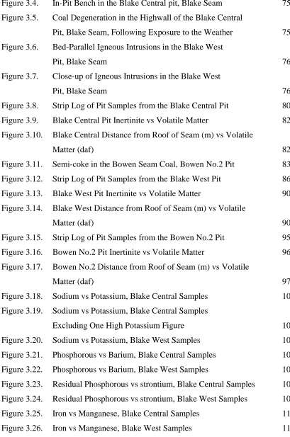
(23) xx Figure 3.4.. In-Pit Bench in the Blake Central pit, Blake Seam. Figure 3.5.. Coal Degeneration in the Highwall of the Blake Central Pit, Blake Seam, Following Exposure to the Weather. Figure 3.6.. 75. Bed-Parallel Igneous Intrusions in the Blake West Pit, Blake Seam. Figure 3.7.. 75. 76. Close-up of Igneous Intrusions in the Blake West Pit, Blake Seam. 76. Figure 3.8.. Strip Log of Pit Samples from the Blake Central Pit. 80. Figure 3.9.. Blake Central Pit Inertinite vs Volatile Matter. 82. Figure 3.10.. Blake Central Distance from Roof of Seam (m) vs Volatile Matter (daf). 82. Figure 3.11.. Semi-coke in the Bowen Seam Coal, Bowen No.2 Pit. 83. Figure 3.12.. Strip Log of Pit Samples from the Blake West Pit. 86. Figure 3.13.. Blake West Pit Inertinite vs Volatile Matter. 90. Figure 3.14.. Blake West Distance from Roof of Seam (m) vs Volatile Matter (daf). 90. Figure 3.15.. Strip Log of Pit Samples from the Bowen No.2 Pit. 95. Figure 3.16.. Bowen No.2 Pit Inertinite vs Volatile Matter. 96. Figure 3.17.. Bowen No.2 Distance from Roof of Seam (m) vs Volatile Matter (daf). 97. Figure 3.18.. Sodium vs Potassium, Blake Central Samples. 101. Figure 3.19.. Sodium vs Potassium, Blake Central Samples Excluding One High Potassium Figure. 101. Figure 3.20.. Sodium vs Potassium, Blake West Samples. 102. Figure 3.21.. Phosphorous vs Barium, Blake Central Samples. 105. Figure 3.22.. Phosphorous vs Barium, Blake West Samples. 106. Figure 3.23.. Residual Phosphorous vs strontium, Blake Central Samples. 106. Figure 3.24.. Residual Phosphorous vs strontium, Blake West Samples. 107. Figure 3.25.. Iron vs Manganese, Blake Central Samples. 112. Figure 3.26.. Iron vs Manganese, Blake West Samples. 113.
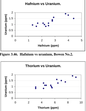
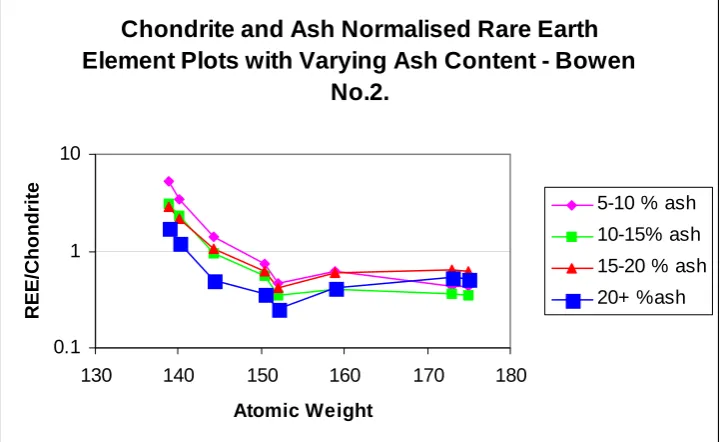
(24) xxi Figure 3.27.. Residual Iron Left After Siderite Calculation vs Sulphur, Blake Central Samples. Figure 3.28.. Residual Iron Left After Siderite Calculation vs Sulphur, Blake West Samples. Figure 3.29.. 115. Ash vs Residual Sulphur Left After Pyrite Calculation, Blake Central Samples. Figure 3.30.. 114. 115. Ash vs Residual Sulphur Left After Pyrite Calculation, Blake West Samples. 116. Figure 3.31.. Iron vs Magnesium, Blake Central Samples. 117. Figure 3.32.. Iron vs Magnesium, Blake West Samples. 117. Figure 3.33.. Iron vs Total Sulphur, Bowen No.2 Samples. 122. Figure 3.34.. Ash vs Total Sulphur, Bowen No.2 Samples. 122. Figure 3.35.. Residual Iron vs Manganese, Bowen No.2 Samples. 124. Figure 3.36.. Residual Iron vs Magnesium, Bowen No.2 Samples. 124. Figure 3.37.. Residual Iron vs Titanium, Bowen No.2 Samples. 125. Figure 3.38.. Hafnium vs Uranium, Blake Central. 138. Figure 3.39.. Hafnium vs Uranium, Blake West. 139. Figure 3.40.. Thorium vs Uranium, Blake Central. 139. Figure 3.41.. Thorium vs Uranium, Blake West. 139. Figure 3.42.. Ash vs Tungsten, Blake Central. 141. Figure 3.43.. Ash vs Tungsten, Blake West. 141. Figure 3.44.. Chondrite and Ash normalised REE concentration, Blake Central. 142. Figure 3.45.. Chondrite and Ash normalised REE concentration, Blake West.. 143. Figure 3.44.. Hafnium vs Uranium, Bowen No.2. 149. Figure 3.47.. Thorium vs Uranium, Bowen No.2. 149. Figure 3.48.. Chondrite and Ash normalised REE concentration, Bowen No.2.. 150. Figure 3.49.. Strip Log Showing Vertical Changes in Minerals and Trace Elements in the Blake Central Pit Seam. Figure 3.50.. 157. Strip Log Showing Vertical Changes in Minerals and Trace Elements in the Blake West Pit Seam. 158.
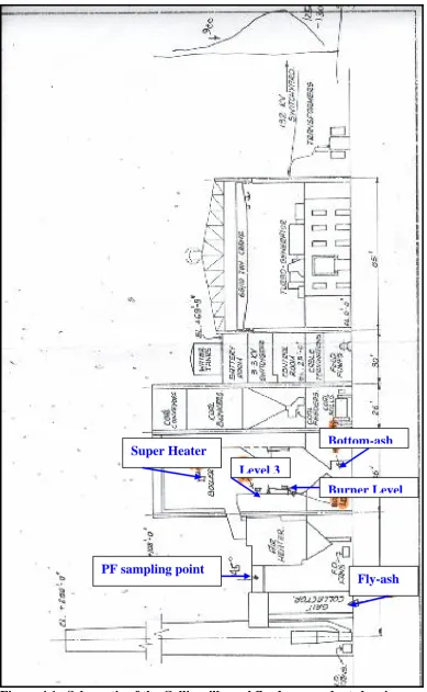
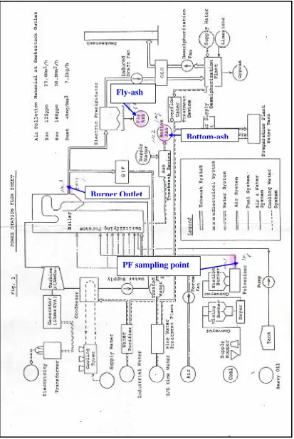
(25) xxii Figure 3.51.. Strip Log Showing Vertical Changes in Minerals and Trace Elements in the Bowen No.2 Pit Seam. 159. Chapter 4.. Figure 4.1.. Schematic of the Collinsville Coal Fired Power Plant. 172. Figure 4.2.. Schematic of the Mitsui Mining Coal Fired Power Plant. 173. Figure 4.3.. Positions for Isokinetic Sampling. 174. Figure 4.4.. INAA/ XRF Results vs the USGS Results for Collinsville Pulverised Fuel. Figure 4.5.. 176. INAA/ XRF Results vs MW-ICP-MS Results for Japanese Pulverised Fuel. 177. Figure 4.6.. Proportions of Antimony Leached. 183. Figure 4.7.. Proportions of Arsenic Leached. 185. Figure 4.8.. Proportions of Barium Leached. 186. Figure 4.9.. Proportions of Beryllium Leached. 187. Figure 4.10.. Proportions of Boron Leached. 188. Figure 4.11.. Proportions of Chromium Leached. 189. Figure 4.12.. Proportions of Cobalt Leached. 190. Figure 4.13.. Proportions of Copper Leached. 191. Figure 4.14.. Proportions of Lead Leached. 191. Figure 4.15.. Proportions of Manganese Leached. 192. Figure 4.16.. Proportions of Nickel Leached. 193. Figure 4.17.. Proportions of Selenium Leached. 194. Figure 4.18.. Proportions of Tin Leached. 195. Figure 4.19.. Proportions of Uranium Leached. 195. Figure 4.20.. Proportions of Vanadium Leached. 196. Figure 4.21.. Proportions of Zinc Leached. 197. Figure 4.22.. Proportions of Cadmium and Molybdenum Leached. 198. Figure 4.23.. Proportions of Rare Earth Elements Leached. 199.
(26) xxiii Figure 4.24.. Proportions of Aluminium, Bromine & Phosphorous Leached. 200. Figure 4.25.. Proportions of Row 4 Transition Metals Leached. 201. Figure 4.26.. Proportions of Heavy Metals Leached. 203. Figure 4.27.. Proportions of Group I and II Elements Leached. 205. Chapter 5.. Figure 5.1.. The Collinsville Coal Fired Power Station. 214. Figure 5.2.. Relative Enrichment of Silicon. 221. Figure 5.3.. Relative Enrichment of Aluminium. 221. Figure 5.4.. Relative Enrichment of Iron. 222. Figure 5.5.. Relative Enrichment of Magnesium. 223. Figure 5.6.. Relative Enrichment of Sodium. 223. Figure 5.7.. Relative Enrichment of Titanium. 225. Figure 5.8.. Relative Enrichment of Manganese. 225. Figure 5.9.. Relative Enrichment of Phosphorous. 225. Figure 5.10.. Relative Enrichment of Sulphur. 226. Figure 5.11.. Relative Enrichment of Gold. 227. Figure 5.12.. Relative Enrichment of Arsenic. 227. Figure 5.13.. Relative Enrichment of Boron. 228. Figure 5.14.. Relative Enrichment of Barium. 229. Figure 5.15.. Relative Enrichment of Cobalt. 229. Figure 5.16.. Relative Enrichment of Chromium. 230. Figure 5.17.. Relative Enrichment of Copper. 231. Figure 5.18.. Relative Enrichment of Caesium. 231. Figure 5.19.. Relative Enrichment of Mercury. 232. Figure 5.20.. Relative Enrichment of Molybdenum. 233. Figure 5.21.. Relative Enrichment of Nickel. 233. Figure 5.22.. Relative Enrichment of Lead. 234. Figure 5.23.. Relative Enrichment of Rubidium. 235.
(27) xxiv Figure 5.24.. Relative Enrichment of Antimony. 235. Figure 5.25.. Relative Enrichment of Selenium. 236. Figure 5.26.. Relative Enrichment of Tin. 237. Figure 5.27.. Relative Enrichment of Thorium. 238. Figure 5.28.. Relative Enrichment of Uranium. 238. Figure 5.29.. Relative Enrichment of Vanadium. 239. Figure 5.30.. Relative Enrichment of Tungsten. 240. Figure 5.31.. Relative Enrichment of Zinc. 240. Figure 5.32.. Relative Enrichment of Cerium. 241. Figure 5.33.. Relative Enrichment of Europium. 242. Figure 5.34.. Relative Enrichment of Hafnium. 242. Figure 5.35.. Relative Enrichment of Iridium. 243. Figure 5.36.. Relative Enrichment of Lanthanum. 243. Figure 5.37.. Relative Enrichment of Lutetium. 244. Figure 5.38.. Relative Enrichment of Neodymium. 244. Figure 5.39.. Relative Enrichment of Scandium. 245. Figure 5.40.. Relative Enrichment of Samarium. 245. Figure 5.41.. Relative Enrichment of Strontium. 246. Figure 5.42.. Relative Enrichment of Tantalum. 246. Figure 5.43.. Relative Enrichment of Terbium. 247. Figure 5.44.. Relative Enrichment of Ytterbium. 247. Chapter 5.. Figure 6.1.. Bowen Coke Works. Figure 6.2.. Quality Parameters of Coal Delivered to the Bowen. 255. Coke Works During Time of Sampling. 256. Figure 6.3.. Concentration of Silicon in Feed Coal and Coke with Time. 258. Figure 6.4.. Silicon CRE for Coke and Breeze with Time. 258. Figure 6.5.. Concentration of Aluminium in Feed Coal and Coke with Time. 259.
(28) xxv Figure 6.6.. Aluminium CRE for Coke and Breeze with Time. 259. Figure 6.7.. Concentration of Iron in Feed Coal and Coke with Time. 260. Figure 6.8.. Iron CRE for Coke and Breeze with Time. 260. Figure 6.9.. Concentration of Sodium in Feed Coal and Coke with Time. 261. Figure 6.10.. Sodium CRE for Coke and Breeze with Time. 261. Figure 6.11.. Concentration of Titanium in Feed Coal and Coke with Time. 262. Figure 6.12.. Titanium CRE for Coke and Breeze with Time. 262. Figure 6.13.. Concentration of Manganese in Feed Coal and Coke with Time. 263. Figure 6.14.. Manganese CRE for Coke and Breeze with Time. 263. Figure 6.15.. Concentration of Phosphorous in Feed Coal and Coke with Time. 264. Figure 6.16.. Phosphorous CRE for Coke and Breeze with Time. 264. Figure 6.17.. Concentration of Sulphur in Feed Coal and Coke with Time. 265. Figure 6.18.. Sulphur CRE for Coke and Breeze with Time. 265. Figure 6.19.. Concentration of Gold in Feed Coal and Coke with Time. 266. Figure 6.20.. Gold CRE for Coke and Breeze with Time. 266. Figure 6.21.. Concentration of Arsenic in Feed Coal and Coke with Time. 267. Figure 6.22.. Arsenic CRE for Coke and Breeze with Time. 267. Figure 6.23.. Concentration of Barium in Feed Coal and Coke with Time. 268. Figure 6.24.. Barium CRE for Coke and Breeze with Time. 268. Figure 6.25.. Concentration of Bromine in Feed Coal and Coke with Time. 269. Figure 6.26.. Bromine CRE for Coke and Breeze with Time. 269. Figure 6.27.. Concentration of Cobalt in Feed Coal and Coke with Time. 270. Figure 6.28.. Cobalt CRE for Coke and Breeze with Time. 270. Figure 6.29.. Concentration of Chromium in Feed Coal and Coke with Time. 271. Figure 6.30.. Chromium CRE for Coke and Breeze with Time. 271. Figure 6.31.. Concentration of Caesium in Feed Coal and Coke with Time. 272. Figure 6.32.. Caesium CRE for Coke and Breeze with Time. 272. Figure 6.33.. Concentration of Hafnium in Feed Coal and Coke with Time. 273. Figure 6.34.. Hafnium CRE for Coke and Breeze with Time. 273. Figure 6.35.. Concentration of Molybdenum in Feed Coal and Coke with Time 274. Figure 6.36.. Concentration of Nickel in Feed Coal and Coke with Time. 275.
(29) xxvi Figure 6.37.. Concentration of Rubidium in Feed Coal and Coke with Time. 276. Figure 6.38.. Concentration of Antimony in Feed Coal and Coke with Time. 276. Figure 6.39.. Antimony CRE for Coke and Breeze with Time. 277. Figure 6.40.. Concentration of Selenium in Feed Coal and Coke with Time. 277. Figure 6.41.. Selenium CRE for Coke and Breeze with Time. 278. Figure 6.42.. Concentration of Strontium in Feed Coal and Coke with Time. 278. Figure 6.43.. Strontium CRE for Coke and Breeze with Time. 279. Figure 6.44.. Concentration of Thorium in Feed Coal and Coke with Time. 279. Figure 6.45.. Thorium CRE for Coke and Breeze with Time. 280. Figure 6.46.. Concentration of Uranium in Feed Coal and Coke with Time. 280. Figure 6.47.. Uranium CRE for Coke and Breeze with Time. 281. Figure 6.48.. Concentration of Tungsten in Feed Coal and Coke with Time. 281. Figure 6.49.. Tungsten CRE for Coke and Breeze with Time. 282. Figure 6.50.. Concentration of Zinc in Feed Coal and Coke with Time. 282. Figure 6.51.. Zinc CRE for Coke and Breeze with Time. 283. Figure 6.52.. Concentration of Cerium in Feed Coal and Coke with Time. 283. Figure 6.53.. Concentration of Europium in Feed Coal and Coke with Time. 284. Figure 6.54.. Concentration of Lanthanum in Feed Coal and Coke with Time. 284. Figure 6.55.. Concentration of Lutetium in Feed Coal and Coke with Time. 284. Figure 6.56.. Concentration of Neodymium in Feed Coal and Coke with Time. 285. Figure 6.57.. Concentration of Scandium in Feed Coal and Coke with Time. 285. Figure 6.58.. Concentration of Samarium in Feed Coal and Coke with Time. 285. Figure 6.59.. Concentration of Tantalum in Feed Coal and Coke with Time. 286. Figure 6.60.. Concentration of Terbium in Feed Coal and Coke with Time. 286. Figure 6.61.. Concentration of Ytterbium in Feed Coal and Coke with Time. 286. Figure 6.62.. Cerium CRE for Coke and Breeze with Time. 287. Figure 6.63.. Europium CRE for Coke and Breeze with Time. 287. Figure 6.64.. Lanthanum CRE for Coke and Breeze with Time. 288. Figure 6.65.. Lutecium CRE for Coke and Breeze with Time. 288. Figure 6.66.. Neodymium CRE for Coke and Breeze with Time. 288. Figure 6.67.. Scandium CRE for Coke and Breeze with Time. 289.
(30) xxvii Figure 6.68.. Samarium CRE for Coke and Breeze with Time. 289. Figure 6.69.. Tantalum CRE for Coke and Breeze with Time. 289. Figure 6.70.. Terbium CRE for Coke and Breeze with Time. 290. Figure 6.71.. Ytterbium CRE for Coke and Breeze with Time. 290. Chapter 9.. Figure 9.1.. Collinsville Coalmine Pit Sample Summary.. 342. Figure 9.2.. Coal Utilisation Summary Diagram - Combustion.. 347. Figure 9.3.. Coal Utilisation Summary Diagram – Combustion & Carbonisation.. 350.
(31) xxviii. List of Tables. Chapter 1.. Table 1.1.. Coal Ash Chemistry and Slagging/ Fouling Characteristics. 5. Table 1.2.. Trace Elements of Environmental Interest. 9. Table 1.3.. Content of Environmentally Significant Trace Elements in World Coals. Table 1.4.. 12. Likely Trace Element Mode of Occurrence from Literature Scores. Table 1.5.. 14. Percentage of Coal Ash from Various Combustion Configurations. 32. Table 1.6.. Element Partitioning Class Comparison. 34. Table 1.7.. Distribution of Elements Among Bottom Ash, Fly Ash and Flue Gas. 35. Chapter 2.. Table 2.1.. Analytical Methods used in this Study. 52. Table 2.2.. INAA Element Detection Limits. 54. Table 2.3.. Repeat Analysis by INAA. 56. Table 2.4.. Comparison of Ash Percent, Proximate and 400oC Ashing Methods. 61. Chapter 3.. Table 3.1.. Interpretation of Depositional Environment from Coal Characteristics. 91.
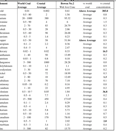
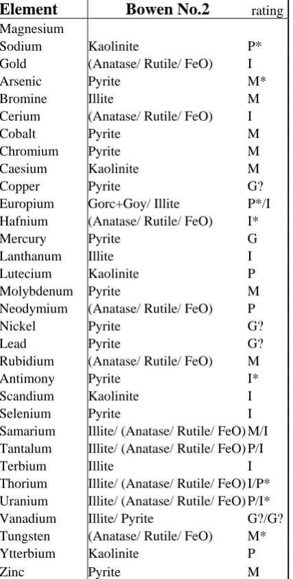
(32) xxix Table 3.2.. Residual Phosphorous in Blake Central Samples following Normative Calculations.. Table 3.3.. Residual Phosphorous in Blake West Samples following Normative Calculations.. Table 3.4.. 108. 109. Residual Phosphorous in Bowen No.2 Samples following Normative Calculations.. 120. Table 3.5.. Normative Mineral Assemblage (ppm) – Blake Central Samples. 127. Table 3.6.. Normative Mineral Assemblage (ppm) – Blake West Samples. 128. Table 3.7.. Normative Mineral Assemblage (ppm) – Bowen No.2 Samples. 129. Table 3.8.. Comparison of XRD and Normative Mineral Assemblages. 130. Table 3.9.. Concentration of Trace Elements in the Blake Seam Compared to World Coal and Crustal Averages. 133. Table 3.10.. Mode of Occurrence of Trace Elements in the Blake Seam. 136. Table 3.11.. Concentration of Trace Elements in the Bowen Seam Compared to World Coal and Crustal Averages. 144. Table 3.12.. Mode of Occurrence of Trace Elements in the Bowen Seam. 146. Table 3.13.. Weighted Average Trace Element Concentration in Heat Affected and Unaffected Samples. 154. Chapter 4.. Table 4.1.. Analysis Results for Collinsville and Japanese Pulverised Fuel Samples by Analysis Method. 178. Table 4.2.. Raw Sequential Leaching Results. 180. Table 4.3.. Tabulated Mode of Occurrence from Interpretation of Sequential Leach Data.. Table 4.4.. 206. The Proportion of Each Trace Element Leached by Each Reagent and the Absolute Differences between Results for the Two Fuel Samples. 208.
(33) xxx Chapter 5.. Table 5.1.. Elemental Concentrations of Major and Trace Elements in Combustion Plant Solid Waste Streams.. 216. Table 5.2.. Major Element Oxides in Ash. 218. Table 5.3.. Trace Element Classification into 3 Classes Based on their Behaviour During Combustion in the Boiler and Ducts with their Relative Enrichment Factors (RE). Table 5.4.. 219. Partitioning Class of Elements in Collinsville, Mitsui and Literature Example Combustion Plants. 252. Chapter 6.. Table 6.1.. Classification of Elements by Partitioning Behaviour in Carbonisation.. Table 6.2.. 290. Classification of Element Partitioning Behaviour in Carbonisation. Table 6.3.. 293. Trace Element Concentration in Bowen Plant Coke Breeze and World Average Soils. 294. Chapter 7.. Table 7.1.. Trace Element Concentration in Ash and Bottom Ash. 301. Table 7.2.. Water Quality Guideline Values and TCLP Concentrations. 302. Table 7.3.. Analysis of Water from Observation Bores and Duck Pond Adjacent to Collinsville Power Plant Ash Dams. Table 7.4.. 302. Calculated Proportions of Element Mobilised by the TCLP Protocol. 307.
(34) xxxi Chapter 8. Table 8.1.. Comparison of Mode of Occurrence from Graphical and Sequential Leaching Methods. Table 8.2.. Significant Differences in Mode of Occurrence Related to Volatility and Leachability. Table 8.3.. Table 8.4.. 311. 323. Trace Element Mode of Occurrence and Partitioning Behaviour in Combustion and Carbonisation. 332. Absolute Difference Between Breeze CRE Figures. 337.
(35) xxxii. List of Appendices. Appendix 1.. Health Effects of Trace Elements. 381. Appendix 2.. Mode of Occurrence of Trace Elements in Coal. 397. Appendix 3.. Maceral and Ro(max) Analysis Results. 429. Appendix 4.. Proximate and Elemental Analysis Results for Collinsville Channel Samples. 435. Appendix 5.. XRD Analysis of Low Temperature Ash. 445. Appendix 6.. Graphs to Determine Mode of Occurrence of Trace Elements in Blake Central, Blake West and Bowen No.2 Pits. Appendix 7.. 448. Proximate and Elemental Analysis Results for Bowen Coke Works Samples. 494.
(36) Chapter 1.. Literature Review.. 1.0.. Chapter Resume.. Chapter 1 comprises a short introduction to trace elements in coal and coal utilisation, presenting a review of pertinent published literature and outlining the major reasons for the surge of interest in this topic. The chapter covers a number of different aspects, including health effects, concentration, mode of occurrence and geological aspects of trace elements in coal, as well as the behaviour of trace elements in combustion and leachability of fly-ash.. 1.1.. Introduction.. In a competitive marketing environment (Knapp, 1999), detailed knowledge of coal quality may be a deciding factor in marketing success. Information on the concentration of key trace elements in a prospective coal may be required by the purchaser to better manage increasingly strict environmental impact requirements and for price bargaining. Studies of trace elements in coal are, therefore, impelled by both financial and environmental concerns.. At present, the majority of coal mined is combusted for electricity generation or carbonised to produce metallurgical coke. Liquefaction and gasification of coal, although historically important, are currently of minor importance (although this could change). The suitability of a coal for use in the major utilisations can be divided into limitations governed by the organic, and the inorganic, constituents of the coal.. The elements carbon, hydrogen, nitrogen, oxygen and sulphur are generally considered to make up the organic fraction of the coal, although this is not always valid (Daniels and Altaner, 1993). The industrial properties of the organic fraction of coal are controlled by coal rank and coal type. Coal rank is the degree coalification (ie the degree of physical and chemical change) the degraded plant material has undergone along a continuum from the peat stage to the meta-anthracite stage. The degree of coalification depends mainly on the maximum temperature surrounding.
(37) rocks have attained and the period for which it is maintained, and pressure, which may retard chemical reactions but promotes physical changes (such as loss of porosity and alignment of structural units).. However, the organic chemistry of individual coals of the same rank may be radically different, these differences being due to coal type. Coal type is determined, in the “classical” sense, by the proportions of the various macerals in the coal (ie the proportion of inertinite, vitrinite and liptinite, and by implication, sub-macerals thereof). The chemistry of each maceral group differs from the others. Liptinite is less aromatic than vitrinite, containing a higher proportion of aliphatic groups and correspondingly higher hydrogen (Teichmüller et al., 1998). Inertinite is more aromatic than vitrinite, containing more carbon but with very low hydrogen contents (Teichmüller et al., 1998). The chemistry of vitrinite is intermediate between chemistry of the liptinite and the inertinite groups. Variations in the proportions of the maceral groups in different coals would clearly result in very different chemical properties. For example, some Australian coals (eg Blair Athol, some Lithgow seams, Coorabin) are relatively low in vitrinite and high in inertinite and, consequently, are considered sub-hydrous (low in hydrogen) (Suggate, 1998).. A second type-controlled variation in coal chemistry may be caused by variation in the chemistry sub-macerals, particularly the vitrinite sub-macerals. Telocollinite (now called collotelinite) (International Committee for Coal and Organic Petrology, 1998) and telinite are woody vitrinite sub-macerals exhibiting a slightly higher reflectance than desmocollinite (now called collodetrinite) (International Committee for Coal and Organic Petrology, 1998) which may contain fine lipoid (liptinitic) inclusions.. A third type-controlled variation in coal chemistry is caused by variations in the chemistry of a single sub-maceral (eg telocollinite/ telovitrinite) (Newman, 1985; Newman, 1991; Newman et al., 1991). In such cases it is thought that the vitrinite absorbs hydrogen or hydrogen-rich substances. Coal type may be a reflection of the depositional environment of the precursor peat, but the relationships are complex..
(38) Rank and type determine which utilisation process is most suitable for a particular coal. For example, coking coals are generally required to have moderate to high thermoplasticity, high Free Swelling Index (FSI) figures (~5 plus) and, ideally, a Coke Strength after Reaction (CSR) between 57 & 75. These properties are mostly governed by rank, prime coking coals having a vitrinite reflectance of between Ro(max) 1.2% & 1.4% (ACIRL, 1996; Diessel, 1998), but coal type (Quick, 1992; Rentel, 1987), and inorganic content and composition (see below) also exert a strong influence. Steaming coal requirements are broader and depend in part on plant design and operating conditions. However, good thermal coals are generally of lower rank, such coals being easier to ignite and giving greater flame stability due to the higher volatile matter content. Further, low rank coals have a higher rate of char burnout due to the less ordered carbon structure of the coal (Diessel, 1998) and greater porosity that allows easier ingress of combustive gasses. Coal rank also exerts some control on the grindability (HGI) of a thermal coal (Diessel, 1998; Hower and Parekh, 1991).. The inorganic constituents of the coal may limit utilization by negatively impacting on the industrial process or plant, and/ or by production of environmental pollutants in gases or from solid wastes. Ash constituents and some element information will often be required before a customer commits to buying a given coal. In general the elemental analyses requested are a reflection of utilization impact concerns. For example, the ratio of acidic to basic constituents in the coal ash will influence the fusion temperature of the ash (AFT) (Couch, 1994; Gray, 1987; Moore and Fergusson, 1997; Vuthaluru, 1999). A number of indexes have been devised to assess the impact of the acidic/ basic ratio on combustion processes, eg slagging index, fouling index (Table 1.1.). “High” concentrations of chlorine, fluorine, and vanadium in the feed coal may cause corrosion of the combustion equipment (Caswell et al., 1984; Liu et al., 2000; Shearer et al., 1997; Spears and Zheng, 1999). High vanadium coals may cause agglomeration in fluidised bed combustion boilers (Anthony and Jia, 2000). In carbonisation, basic elements can catalyse reduction reactions in the blast furnace, increasing coke consumption and production of breeze, and reducing coke strength and porosity (Coin, 1995; Diessel, 1998; Gunn, 1988). A 1% increase in the concentration of sulphur is thought to increase the coke consumption rate by as much as 32 kg per net ton of hot metal (Zimmerman, 1979) and greatly increase the production of slag. Phosphorous in coking coals also contributes to the slag, but most.
(39) will eventually end up in the product steel (Ward et al., 1996) making it brittle (Dennis, 1963; Moore and Moore, 1999). Boron in coking coal also ends up in the steel and causes brittleness (Swaine, 1990).. Inorganic constituents may also have an adverse effect on the environment (ignoring possible greenhouse effects caused by CO2 from combustion of the organic matter). Increasing attention is now being given to the potential environmental impact of trace elements released by coal utilization. It has long been known that sulphur from coal combustion can cause acid rain (Bouska and Pesek, 1999). Similarly chlorine and fluorine in coal can also cause acidic emissions. A number of studies have shown that trace elements from coal combustion and combustion residues increase the concentration of toxic elements in the biosphere, in some cases resulting in negative health impacts on plants, animals and humans, (Agrawal et al., 1993; Bencko and Symon, 1977a; Bencko and Symon, 1977b; Clark et al., 1999; Finkelman, 1993; Gupta, 1999; Gutenmann and Bache, 1976; Huggins et al., 1999; Klusek et al., 1993; Knott et al., 1985; Panov et al., 1999; Swaine, 1989; Swaine, 1990; Swaine and Goodarzi, 1995; Wadge and Hutton, 1986; Zheng et al., 1999). Trace elements may be detrimental if intake or exposure is present at concentrations less than or greater than the optimum range (Swaine and Goodarzi, 1995) (Figure 1.1.) for a given organism, toxicity depending also on speciation (Huggins et al., 1999), organism tolerance (Bowen, 1966), and element antagonism or synergism (Kizilshtein and Kholodkov, 1999; Swaine, 1995; Wood, 1974) (Appendix 1). The concern is that the release of trace elements from coal utilization will result in elemental concentrations exceeding the toxicity threshold of some plants and animals (including humans)..
(40) THIS TABLE HAS BEEN REMOVED DUE TO COPYRIGHT RESTRICTIONS.
(41) THIS IMAGE HAS BEEN REMOVED DUE TO COPYRIGHT RESTRICTIONS. Figure 1.1. General Representation of the Effects of Increases of Concentration of a Trace Element. Source Swaine & Goodarzi (1995).. The widespread availability of large coal resources, coupled with decreasing opportunities to dam rivers for hydroelectric power generation, and the social unacceptability of nuclear power, suggest that coal consumption, for energy generation at least, will increase for some decades to come, particularly in developing countries (eg China, India) (Fyfe, 1999). Some coals mined in these developing countries are notable for a higher than “average” concentration of environmentally hazardous trace elements, eg Chinese coals, see Table 1.3., (Ren et al., 1999). Japanese power companies are now formulating standards as to the maximum allowable concentration of trace elements in supplied coal (Nishioka, Mitsui Mining; pers com, 1999).. Although the impact of some trace elements on animal and plant health is currently the prime impetus for studying trace elements in coal, there are other potential reasons for interest. Depending on concentration and distribution, trace elements may also be a source of economic by-products (Seredin, 1996), of use in prospecting for ore deposits, for soil amelioration, and for seam correlation purposes (Finkelman, 1993)..
(42) The use of trace element data in characterizing coals already mined is of little use for the prediction of future environmental impacts because the inhomogeneity, even within a seam, of elemental contents precludes meaningful extrapolation to new seams and mining blocks (see below). Therefore, trace element studies will need to be ongoing with mine development and coal use to adequately monitor element concentrations in the current product..
(43) 1.2.. Trace Elements of Environmental Interest in Coal.. Trace elements are only of environmental concern if there is some recognisable impact on the health and well being of the ecosystem. However it is recognised that the impact of some trace elements may not be clinically detectable, or make take years or decades to become apparent. It should be noted that “health impact” is not anthropocentric in nature, and any negative impact on any part of the biosphere is generally viewed as undesirable by local, regional and national authorities as well as by the public. Any emphasis on human health impacts in this document are, therefore, merely a reflection of the literature reviewed.. It is notable that many of the trace elements listed as potentially environmentally deleterious if they are concentrated to toxic levels by coal utilisation are essential in low concentrations for the growth and well being of plants and animals. There is potential for trace elements from coal combustion waste to provide environmentally useful by-products if managed properly. For example, there is some potential to use fly-ash as a soil ameliorant to add essential elements to deficient soils (Finkelman, 1993), although studies need to be undertaken to ensure that the acid conditions of the soil will not release toxic cations from the fly-ash (Jones, 1995).. Four groups of environmentally significant elements are recognised (Swaine and Goodarzi, 1995; Zhang et al., 2004) (Table1.2.). Group I elements are known to be hazardous in some circumstances, although the concentration of these elements is known to be low in most coals. Group IIA includes the elements B, Mn and Mo, which should be taken into consideration in leachates from wastes or during mine reclamation, and chlorine, which can cause acid emissions. Group IIB elements are unlikely to cause problems, although the radioactive elements U and Th should clearly be kept to a minimum. Group III elements are not expected to cause problems in the concentrations given for most coals..
(44) Table 1.2. Trace Elements of Environmental Interest. (1995). I As Cd Cr Hg Se. IIA B Cl F Mn Mo Ni Pb. IIB Be Cu P Th U V Zn. From Swaine & Goodarzi. III Ba Co Sb Sn Tl. The health impacts of the environmentally significant trace elements listed in Table 1.2. are detailed in Appendix 1 along with comments about the essentiality, toxic effects and any synergistic or antagonistic interactions a particular element might have.. Predicting the toxicity of an element in the biosphere is not a simple matter of presence, or indeed of elemental concentration. An organism’s diet, source of exposure, synergistic and antagonistic element interactions, elemental speciation, and tolerance variations between species all play an important role in determining any adverse effects caused by element absorption. Further, some poisons such as lead are cumulative so environmental and health impacts may not be immediately apparent. Hazard and risk assessment requires that even hazards perceived as having a low probability but with potentially significant impact be considered. Because the potential impacts are hard to predict or quantify for the reasons given above, caution is needed when assessing the environmental impact of elements released by coal utilization..
(45) 1.3.. Geological Aspects of Trace Elements in Coal.. 1.3.1. Concentration of Trace Elements in Coal.. 1.3.1.1.. Definitions.. Trace elements are defined as being present in concentrations up to 1000 ppm (0.1 %) dry basis in most coals (Lindahl and Finkelman, 1986; Swaine, 1990). Other authors suggest the upper concentration for an element to be classed as trace is 200 ppm (Mukhopadhyay et al., 1998).. In some cases elements usually considered as “trace” in coal are present in very high concentrations, eg arsenic present at 32,000 ppm and fluorine at 3600 ppm in Chinese coals (Ren et al., 1999); chlorine at 9100 ppm (Swaine, 1995) or 10,000 ppm (Valkovic, 1983a) in UK coals. Elements present in such concentrations could hardly be considered trace for the coal concerned. Knowledge of the concentration of trace elements in a coal can be important when comparing coals for purchase if such high levels might cause undue environmental impacts or be detrimental in utilisation.. A trace element is defined here as an element present in most coals in concentrations less than 1000ppm.. 1.3.1.2.. Comparison of Trace Element Concentrations.. For most coals, the concentration of trace elements is no higher than that of soils and shales (Swaine, 1989; Swaine, 1990) (exceptions being selenium, germanium, molybdenum and lead), and lower in many trace elements than some fertilizers. Swaine (1995) states that “coals with unusually high contents of trace elements must not be forgotten because these are the ones that may give problems during mining and usage” (Swaine, 1989; Swaine, 1990; Swaine, 1995). While the concentration of trace elements in most coals may be similar to soils and shales, the combustion of coal concentrates some elements in solid waste fractions (which must be disposed of) and emits others to the atmosphere as a point source over a long period of time. Some elements such as lead may accumulate in the environment over time, so the long-term impacts of using a particular coal may not be immediately apparent..
(46) Average values of trace element concentration can be difficult to use as a basis for comparing coals due to the inhomogeneity elemental distribution, even within a single seam (Swaine, 1995). Inhomogeneity is caused by the complex geochemical controls on trace element concentration and distribution, namely “intake of trace element during plant growth, enrichment during plant decay, sedimentation and diagenesis, burial and coalification, and subsequent late-stage mineralization” (Mukhopadhyay et al., 1998). A number of trace elements have been shown to have a log frequency distribution so a geometric mean may be more useful when comparing coals (Bouska and Pesek, 1999; Swaine, 1995; White et al., 1989). The concentration range of trace elements in coal mined from New South Wales and Queensland mines is generally similar over time, so useful comparisons may be made between data sets showing a concentration range (Swaine, 1995). Table 1.3. shows the range of trace element contents published for a number of world coals by country. Another method for comparing the trace element contents of coals is to use an independent ‘yard stick’. Comparison of “Clarke Values” (average concentration of the element in the earths crust), eg (Taylor, 1964), with coal elemental analysis results indicate the enrichment or depletion of a given element compared to the earths crust (Faure, 1991; Skinner and Porter, 1987); examples include (Beaton et al., 1991), (Casagrande and Erchull, 1977), (Eskenazy, 1982), (Goodarzi, 1987b) and (Goodarzi, 1988). Rare earth elements may be converted to a chondrite normalised basis in order to assess enrichment or depletion of the element; examples include (Birk and White, 1991), (Eskenazy, 1987) and (Seredin, 1996)..
(47) Table 1.3. - Content of Environmentally Significant Trace Elements in World Coals.. THIS TABLE HAS BEEN REMOVED DUE TO COPYRIGHT RESTRICTIONS. (1) Zubovic et al (1980); (2) Clark and Swaine (1962), Swaine (1977); (3) mostly from Goodarzi and co-workers; (4) several (cited by Swaine, 1990) (5) Ren et al. (1999); aDale and Lavrencic (1993) Table based on Swaine (1995).. Because the concentration and redistribution of elements occurs during industrial utilization processes, some workers, e.g. (Toole-O'Neil et al., 1999) have suggested that it may be of practical benefit to compare coals on an equal energy basis. The logic behind this suggestion is that, for example, while a prospective lignite fuel may contain a lower concentration of elements of concern than an alternative bituminous coal, the additional coal consumed to provide the same quantity of energy could result in a greater total volume of deleterious elements being released to the environment. (NB Low rank coals may also have more elements loosely bound to the organic coal structure as cations, which may be more readily released to the atmosphere during combustion)..
(48) 1.3.2. Mode of Occurrence.. 1.3.2.1.. Introduction.. The mode of occurrence of a trace element in coal is important in anticipating the behaviour of the element during coal cleaning, combustion, and weathering and leaching of coal and utilisation waste products (Finkelman, 1993; Finkelman, 1995; Mukhopadhyay et al., 1996; Mukhopadhyay et al., 1999; Querol et al., 1995). The use of a coal with a low concentration of a particular trace element could still result in a detrimental environmental impact if the mode of occurrence allows the element to be readily released during utilisation.. A large number of papers provide mode of occurrence data for coals from around the world (Appendix 2, Table 1.4.), providing a good survey of the most common and, therefore, most likely modes of occurrence for an element. Appendix 2 lists the elements of environmental interest from Table 1.2., and scores the modes based on the number of papers in which that mode was encountered (a full description of the scoring method can be found in Appendix 2). Table 1.4. is a summary of the mode of occurrence score results. The mode of occurrence scores provide an additional aid to the interpretation of new analytical results in this study..
(49) Table 1.4., Likely Trace Element Mode of Occurrence from Literature Scores. Element Organic Inorganic Sulphide Clays Carbonate Others Antimony 13 41 36 10 Arsenic 15 14 69 1 1 Barium 21 19 21 35 4 Beryllium 75 25 Boron 81 19 Cadmium 32 68 Chlorine 61 39 Chromium 22 28 30 20 Cobalt 33 19 23 14 6 5 Copper 22 20 38 13 7 Lead 5 13 65 17 Manganese 18 19 10 37 16 Mercury 8 78 14 Molybdenum 34 6 49 11 Nickel 23 11 36 31 Phosphorous 6 94 Selenium 25 7 43 24 Thallium 83 17 Thorium 1 40 59 Tin 9 30 33 28 Uranium 39 32 22 7 Vanadium 30 25 35 10 Zinc 7 16 35 42. 1.3.2.2.. Methods of Determining Modes of Occurrence.. A number of methods to determine or indicate trace element mode of occurrence in coal are described in the literature. No individual method is flawless, so several complementary methods should be used wherever possible to provide a robust mode of occurrence assessment. While some modes of occurrence are more frequently encountered for an element, many have several potential occurrence modes (Table 1.4.). One apparent fact is that a large number of trace elements of environmental concern are either dominantly or sometimes hosted by pyrite; ie, fourteen out of the twenty four trace elements of environmental concern listed in Goodarzi and Swaine (1995); see also (Finkelman, 1979; Spears et al., 1999). The concentration and mode of occurrence of an element in coal depends on a complex set of geological interactions between the “intake of trace elements during plant growth, enrichment during plant decay, sedimentation and diagenesis, burial and coalification, and latestage mineralization” (Mukhopadhyay et al., 1998). Such a complex set of.
(50) circumstances is seldom identical between different locations, so it is no surprise that, as for elemental concentrations, the mode of occurrence varies on a worldwide scale for most elements. Such complexity means that coal deposits need to be studied on a case-by-case basis.. Determination of trace element mode of occurrence in coal has been undertaken in a variety of ways. To follow is a short review of some common methods.. SEM-EDX. A scanning electron microscope equipped with an energy dispersive X-ray detector (SEM-EDX) has been used by some workers to locate and analyse accessory minerals in coal. Therefore, SEM-EDX directly determines the organic and/ or inorganic phase containing the trace element, and the concentration of the trace element in the host. Advantages over other methods include: 1) The accessory mineral matter can be observed and analysed in situ (Finkelman, 1978). Liberation of accessory minerals from coal by ashing, even low temperature radio frequency ashing, may alter the mineral matter composition and form to a greater or lesser degree (Doolan et al., 1985; Finkelman et al., 1984; Mitchell and Gluskoter, 1976; O'Gorman and Walker, 1971). Further, ashing may result in the loss of some volatile trace elements. Only in-situ direct determination using a method such as SEM-EDX avoids alteration issues caused by ashing. 2) The textural features of the mineral matter can be observed and some interpretation made regarding the origin of the grain, ie detrital, authigenic or extra-terrestrial in origin (Finkelman and Stanton, 1978). SEM-EDX has been used by a number of researchers, eg (Beaton et al., 1991; Finkelman, 1980; Mukhopadhyay et al., 1996; Palmer and Filby, 1984; Van Der FlierKeller and Fyfe, 1986), or in combination with other techniques, eg (Vickridge et al., 1990). Similar techniques include ion microprobe analysis (Finkelman et al., 1984) and nuclear microprobe (Vickridge et al., 1990).. Disadvantages in the use of SEM-EDX are that it is not a bulk analysis technique, it is time consuming, and it is labour intensive. Because of these disadvantages, other methods are frequently used for more general studies..
(51) Float-Sink. The float-sink method assumes that elements concentrated in the float fraction are organically bound and elements concentrated in the sink fraction are inorganically bound. The density fractions may be further analysed to determine the mode of occurrence more specifically by: 1) Sequential extraction of the mineral phases (Feng and Hong, 1999; Miller and Given, 1986) 2) XRD or SEM analysis (Mukhopadhyay et al., 1996; Querol et al., 1995; Seredin, 1996; Spears and Martinez-Tarazona, 1993). 3) By graphing trace elements against major elements related to mineral matter species by normative analysis (Newman, 1988; Ward, 1980). 4) By statistical analysis (Querol et al., 2001a).. A further variant is the analysis of the float-sink data for various size fractions of a low temperature radio frequency ash with integration of mineral matter information from XRD and SEM analysis to deduce mode of occurrence (Palmer and Filby, 1984).. The major flaw in the float sink method is that small grains may be rafted up with the lightest density fraction (Finkelman, 1980). The effect of poor liberation makes some elements appear to be organically associated when in fact they are present within fine mineral grains. Problems of mineral alteration in radio frequency ashing (Finkelman et al., 1984) and detection limits for XRD (~0.1 %) (Lewis and McConchie, 1994) may limit the approach of Palmer and Filby (1984).. Statistical/ Graphical. Graphical relationships between trace element concentration and the ash (or 1/ ash) yield for a series of samples (eg from plies in a channel sample) can be used to infer the organic or inorganic affinity of the element. An element is considered organically bound if it maintains almost the same level or decreases with increasing ash yield, but it is considered inorganically bound if its concentration in coal increases with increasing ash yield. If elements are determined on an in-ash basis, then inorganically bound elements would maintain a horizontal trend line, and organically bound elements decrease in proportion to ash yield. (NB there is a problem with loss of.
(52) volatile elements such as mercury during ashing). A large number of authors use the graphical approach, eg (Beaton et al., 1991; Dilles and Hill, 1984; Eskenazy, 1982; Eskenazy, 1987; Eskenazy et al., 1994; Goodarzi, 1987b; Goodarzi, 1987c; Goodarzi and Van Der Flier-Keller, 1988; Grieve and Goodarzi, 1993; Hower and Bland, 1989; Szilágyi, 1971), or 1/ash (Newman et al., 1997).. A more refined graphical method involves graphing the concentration of a mineral or an element representative of a mineral (eg K for illite) in coal against the concentration of the trace elements of interest, eg (Dewison, 1989; Gayer et al., 1999; Mukhopadhyay et al., 1996; Spears and Zheng, 1999; Van Der Flier-Keller and Fyfe, 1986; Ward et al., 1999). Computer programmes are now available to carry out normative analysis with operator input to define the most likely minerals present in a deposit (Ward and Taylor, 1996). Graphical methods using elemental indicators of specific minerals or normative mineralogical concentrations provide a more informative indication of mode of occurrence, however knowledge of the mineral matter is a prerequisite. The second method has been used in conjunction with the float-sink technique to provide better indications of mode of occurrence in separation experiments.. The shortcoming of the graphical technique is that analysis of trace element mode of occurrence is not direct (cf SEM-EDX). Not all graphical relationships necessarily point to a common mineral host. A positive correlation coefficient could simply point to a common source for graphically related elements rather than a common mode of occurrence (Finkelman, 1980; Finkelman, 1993). One example of how this error could arise is documented for vanadium, which was originally organically bound (substituting for magnesium in chlorophyll) (Riley and Saxby, 1986), but was remobilised and became associated with clay minerals during diagenesis (Patterson et al., 1986). Potentially vanadium could show a good inverse correlation with ash yield (indicating an organic association), but the element is actually associated with clay minerals. A second potential source of error could result from the redistribution of elements at low ranks by aquifer water. Mobile elements could end up with a spatial relationship with unrelated detrital material (Brockway et al., 1991). One final problem is that low ash in a sample does not necessarily indicate that the elements are.
Figure
+7


Related documents