Colony dynamics of the green tree ant (Oecophylla smaragdina Fab.) in a seasonal tropical climate

Full text

(1)ResearchOnline@JCU. This file is part of the following reference:. Lokkers, Cornel (1990) Colony dynamics of the green tree ant (Oecophylla smaragdina Fab.) in a seasonal tropical climate. PhD thesis, James Cook University.. Access to this file is available from:. http://eprints.jcu.edu.au/24114/ The author has certified to JCU that they have made a reasonable effort to gain permission and acknowledge the owner of any third party copyright material included in this document. If you believe that this is not the case, please contact ResearchOnline@jcu.edu.au and quote http://eprints.jcu.edu.au/24114/.

(2) COLONY DYNAMICS OF THE GREEN TREE ANT (Oecophylla smaragdina Fab.) IN A SEASONAL TROPICAL CLIMATE.. Thesis submitted by Cornel Lokkers BSc (JCUNQ) in March 1990. for the degree of Doctor of Philosophy in the Department of Zoology, James Cook University of North Queensland..

(3) 1 Acknowledgements.. Many thanks are owed to my supervisors, Prof. Rhondda Jones, and Dr. Bob Taylor, for their advice and encouragement through the long and winding progress of my project. Their assistance has greatly improved this thesis. I am grateful to Dr. Betsy Jackes for identifying tree species inhabited by ants, and reviewing several sections of the manuscript. For development of the electronics for monitoring ant activity, I thank Reg Mercer and John Sweet, of the Electronics Section, James Cook University. Dr. Glen De'ath (Tropical Veterinary Sciences) provided invaluable advice on all matters statistical. A number of people, including Dr. (to be) Jamie Seymour, Dr. Jamie Oliver, and Dr. Bruce Mapstone helped me comprehend the many mysteries of computer technology. Michael Trenerry kindly provided some excellent photographs of green tree ants. I am indebted to Keith Wright for use of his mango tree plantation at Major Creek during my studies, and to the many people who collected green tree ant queens for me. Dave Hausen provided valuable assistance in the field when sampling nests. The research and technical staff. of. Biological Sciences were always a source of help in times of trouble. I must thank my fellow students for their understanding and tolerance, especially during the last months of writing. This study was supported by a Commonwealth Postgraduate Award from 1986 to 1989, and Special Research Grants during 1986, 1987, and 1989..

(4) ii. Frontispiece. Green tree ant major worker in alarm posture. Green tree ants capturing a wasp..

(5) 111 Abstract.. Most previous investigations of the weaver ant genus (Oecophylla) have been conducted in the relatively non-seasonal environment of the wet tropics (e.g. Greenslade, 1971a,b, 1972; Ledoux, 1950, 1954; Majer, 1976,a,b,c; Vanderplank, 1960; Way, 1954a,b). The present study documented substantial seasonal variation in colony structure and functioning of green tree ant. (0. smaragdina) populations in the. seasonally dry tropical climate which characterizes most of northern Australia. The distribution of. 0. smaragdina. within Australia. was. successfully defined by a combination of mean annual rainfall and average minimum temperature, with a curvilinear demarcation between sites with and without ants. Development and survival of ant brood was markedly reduced by low temperatures, especially the larval stage, which had a threshold temperature (when development theoretically stops) of about 17°C. In contrast, the thresholds for eggs and pupae were about 10°C and 7°C, respectively. At higher temperatures, the 2 physical variables probably indirectly limit ant distribution. by. controlling plant density; ants only inhabited sites with woodland or forest vegetation. Colony extents (the numbers of trees occupied by colonies) were much larger in native vegetation than in a nearby mango plantation. This difference was probably due to the greater tree density in the native forest site. No canopy interconnections were available in the mango orchard to promote movements of ants between trees. Inter-tree migration is essential for weaver ant colonies, to disseminate brood.

(6) iv from the nest containing the colony's single egg-producing queen and possibly also to maintain a uniform colony recognition scent. Levels of reproduction in green tree ant colonies were highest during the wet season and early dry season. Sexual forms were present in nests from November until March, and worker brood were most abundant from January until May. Larval and pupal brood levels rose with increasing precipitation up to monthly rainfall figures around 300 mm. Proportions of worker pupae were reduced during periods of. higher. rainfall, probably due to the production of sexuals at this time Colony extents, measured as the number of trees occupied, were smallest in native forest at the end of the dry season in November, and rose while colonies were reproducing. Most colonies reached peak extents in May, when the proportion of flowering trees was highest (and 2 months after the greatest levels of leaf flushing). After May, brood production generally decreased markedly, and colony extents in native vegetation slowly fell, with ants gradually evacuating from peripheral trees into smaller core areas of high tree density. Cycles of colony extent in the mango plantation lagged behind those in native vegetation by 2 to 4 months; maximum extents coincided with mango tree flowering from July, to September. Tended homopteran levels in mango tree leaf samples were high during the flowering and fruiting period, suggesting that colony expansion may be facilitated by the increased availability of honeydew. As colonies expanded, individual nests became smaller and the number of nests (per tree and per colony) increased. Ant distributions were thus dispersed more evenly throughout colonies during this period. This decentralization may improve foraging efficiencies, or may allow increased patrolling of territories when intrusions by other. ant.

(7) V. colonies (both intra and inter-specific) are most likely. Highest levels of prey intake and ant movement from nests did coincide with periods of greatest reproduction and dispersion; however, the causal relations between these factors are unknown. An electronic light beam counter was developed to monitor ant activity (measured as the number of ants leaving and returning from a nest, and standardized between different nests by dividing by the total population of each nest) in native forest over a two year period. from. Net daily activity was greatest during the wet season months. December to March, and lowest in the dry winter period. The magnitude of these seasonal differences was remarkably high; the largest mean activity of 8.83 ants/nest individual/day (in December) was over 10 times the smallest level of 0.501 (in August). Seasonal patterns of activity correlated well with patterns of total prey weight collected by ants. Liquid food intake, measured as the average weight difference of leaving and returning ants, showed a similar, but very. erratic. pattern; factors such as varying forager sizes, honeydew intake inside the nest, and differing physiological conditions of inhabited trees prevented successful quantification of this food source. A consistent circadian pattern of ant activity was observed autumn and winter (March, May, August): activity peaked around dusk, and dropped to a minimum in the early morning before dawn.. This. circadian pattern was less distinct or completely absent during the spring and summer months (October, December, January). Activity was generally correlated with temperature; the fitted parabolic relationship suggested that activity was markedly reduced by low temperatures, but was less affected by higher temperatures. Circadian patterns of activity did not correlate to patterns of.

(8) vi food intake. Most prey was collected during the daylight hours, suggesting that. 0. smaragdina is primarily a visual predator. Honeydew. intake also appeared to be greatest after dawn. Nocturnally active ants may be involved in other tasks, such as brood and young adult transport, colony scent dispersal, and territorial patrolling/guarding. Mango trees with green tree ant populations had more tended homopterans and fewer numbers of most other arthropod groups than adjacent trees without ants. The proportions of leaves with chlorotic scars from homopterans (primarily. Phenacaspis dilata) were greater in. ant-occupied trees. The fractions of leaves with holes from chewing arthropods, and the average area of leaf missing were greater in antfree trees. Crop yields during the study were relatively low. However,. ants. appeared to augment fruit loss in trees with largest crops during the late stages of fruit development, probably by encouraging homopteran populations and so increasing sap loss. Green tree ants also appeared to reduce frugivory by fruit bats, the major predator of mango fruit..

(9) vii. TABLE OF CONTENTS:. ACKNOWLEDGEMENTS. ABSTRACT.. 1.. 2.. 3.. iii. LIST OF FIGURES.. xi. LIST OF PLATES.. xvi. LIST OF TABLES.. xvii. GENERAL INTRODUCTION. 1.1. Nest structure.. 1. 1.2. Colony structure.. 5. 1.3. Diet.. 8. 1.4. Impact of weaver ants on arboreal arthropods.. 10. 1.5. Aims of the present project.. 12. DESCRIPTION OF STUDY SITES.. 13. 2.1. Townsville.. 13. 2.2. Major Creek.. 23. DISTRIBUTIONAL PATTERNS.. 25. 3.1. Introduction.. 25. 3.2. Methods.. 28. 3.3. Results.. 30. 3.3.1. Distribution in Australia.. 30. 3.3.2. Distribution in Townsville.. 35. 3.4. Discussion.. 41.

(10) viii 4.. EARLY COLONY DEVELOPMENT. 4.1. Introduction.. 46. 4.2. Methods.. 48. 4.3. Results.. 52. 4.3.1. Phenology of first brood.. 52. 4.3.2. Developmental rates.. 59. 4.3.3. Success rates.. 63. 4.3.4. Pleometrotic colony founding.. 65. 4.3.5. Colony development after first adult emergence.. 68. Discussion.. 69. COLONY STRUCTURE.. 77. 4.4. 5.. 46. 5.1. Introduction.. 77. 5.2. Methods.. 81. 5.2.1. Colony extent: Tree number and area occupied.. 82. 5.2.2. Nest density and longevity.. 84. 5.2.3. Nest composition.. 85. 5.3. 5.4. Results.. 87. 5.3.1. Colony extent: tree number and area occupied.. 87. 5.3.2. Inter-colony aggression and colony extent.. 95. 5.3.3. Nest density.. 95. 5.3.4. Nest longevity.. 98. 5.3.5. Nest composition.. 98. 5.3.6. Worker morphometrics.. Discussion.. 115 117.

(11) ix. 6.. ACTIVITY AND FOOD INTAKE. 6.1. 6.2. 6.3. 126. Introduction.. 126. 6.1.1. The components of activity.. 126. 6.1.2. Food intake and its measurement.. 128. 6.1.3. Foraging activity.. 134. Methods.. 137. 6.2.1. Activity.. 137. 6.2.2. Food input.. 148. 6.2.3. Ant tagging.. 149. Results.. 152. 6.3.1. Activity counter calibration.. 152. 6.3.2. Comparison of inward and outward flow.. 155. 6.3.3. Field activity patterns.. 161. 6.3.3.1. Yearly and monthly variation.. 161. 6.3.3.2. Monthly and circadian variation.. 164. 6.3.3.3. Circadian variation during each month.. 167. 6.3.3.4. Field activity: A summary.. 181. 6.3.4. Laboratory activity patterns.. 183. 6.3.5. Food intake.. 188. 6.3.5.1. Prey intake.. 188. 6.3.5.2. Liquid food intake.. 195.. 6.3.5.2.1 Assumptions of weight differential method. 195 6.3.5.2.2 Spatial variation in liquid food intake.. 200. 6.3.5.2.3 Patterns of liquid food intake.. 202. 6.3.5.3 Patterns of worker size.. 206. 6.3.5.4 Brood transport.. 211. 6.3.6 Dyed food dispersal.. 211.

(12) 6.4 Discussion.. 214. 6.4.1 Counting by light beam.. 214. 6.4.2 Patterns of activity and food intake.. 216. GREEN TREE ANTS AND MANGO TREES.. 225. 7.1 Introduction.. 225. 7.2 Methods.. 229. 7.3 Results.. 235. 7.3.1 Insect populations.. 235. 7.3.2 Leaf condition.. 246. 7.3.3 Fruit production.. 255. 7.4 Discussion.. 262. FINAL CONCLUSIONS.. 268. 8.1 Factors influencing ant colonies.. 268. 8.2 The impact of ants on the environment.. 273. BIBLIOGRAPHY.. 278. APPENDIX A.. 289. APPENDIX B.. 301.

(13) xi. LIST OF FIGURES. 1.1. Adult forms of. Oecophylla.. 2.1. Map of northern Queensland showing locations of study sites.. 14. 2.2. Climatic patterns in Townsville from January 1985 to May 1989.. 16. 2.3. Map of Townsville study site in May 1988.. 21. 2.4. Map of Major Creek study site in May 1988.. 24. 3.1. World distribution of weaver ants.. 26. 3.2. Australian distribution of. 31. 0. smaragdina.. 3.3. Temperature and rainfall averages of sites with and without ants.. 33. 3.4. Australian distribution of O. smaragdina in relation to forest and woodland vegetation.. 34. 3.5. Distribution of ant colonies around biological sciences building, JCUNQ.. 36. 3.6. Distribution of trees always, sometimes, and never occupied by ants in Townsville study site.. 37. 3.7. Nearest neighbour distances of trees always, sometimes, and never occupied by ants in Townsville study site.. 39. 3.8. Proportions of different tree species always, sometimes, and never occupied by ants in Townsville study site.. 39. 4.1. Design of artificial ant nest.. 51. 4.2. Phenology of first broods of queens at 24°C.. 54. 4.3. Phenology of first broods of queens at 30°C.. 55. 4.4. Phenology of first broods of queens at 35°C.. 56. 4.5. Phenology of first broods of queens at 20°C.. 57. 4.6. Developmental rates of immature stages in first broods.. 60. 4.7. Success rates of first broods at various temperatures.. 64. 4.8. Phenology of first broods of pleometrotic queen groups (2 queens per group).. 67.

(14) xii 5.1. Temporal variation in total number of trees occupied in Townsville study site.. 88. 5.2. Temporal variation in numbers of trees and areas occupied per colony in Townsville study site.. 88. 5.3. Temporal variation in number of trees occupied and tree condition in Major Creek study site .. 90. ,. 5.4. Temporal variation in number of trees occupied and tree condition 92 for four tree species in Townsville study site. 5.5. Temporal variation in number of trees occupied and composite tree status.. 94. 5.6. Regression of percentage of trees occupied on composite tree status.. 94. 5.7. Temporal variation in numbers of trees occupied by 2 conflicting colonies.. 94. 5.8. Temporal variation in nest densities in 2 tree species.. 96. 5.9 - 5.14. Temporal variation in nest composition and climate 5.9. Ciirns. 5.10. Townsville. 5.11. Bowen. 5.12. Proserpine. 5.13. Mackay. 5.14. Yeppoon.. 99 100 101 102 103 104. 5.15. Seasonal pattern in larval proportions.. 108. 5.16. Effect of current month's rainfall on larval proportions.. 108. 5.17. Seasonal pattern in pupal proportions.. 109. 5.18. Effect of previous month's rainfall on pupal proportions.. 109. 5.19. Effect of current month's temperature on pupal proportions.. 109. 5.20. Seasonal pattern in ratio of major to minor worker adults.. 111. 5.21. Effect of previous month's rainfall on ratio of major to minor worker adults.. 111. 5.22. Temporal variation in nest composition in Townsville study site.. 113. 5.23. Relationship of scape lengths and thorax lengths in major and minor worker adults.. 116.

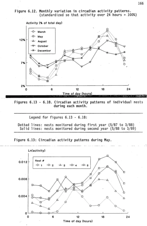
(15) 5.24. Temporal variation in scape lengths of major workers in Townsville study site.. 116. 6.1. Schematic representation of potential trophallactic food flow between foragers feeding on honeydew.. 133. 6.2. Design of light beam counter for measuring ant activity in the field.. 138. 6.3. Design of laboratory ant activity counter system.. 147. 6.4. Design of vacuum-powered ant aspirator.. 147. 6.5. Calibration of ant flow recorded by light beam counter with manually recorded ant flow.. 153. 6.6. Efficiency of light beam ant counter in light and dark conditions.. 153. 6.7. Ant activity recorded by counter from 9.30, 20 May, to 9.10, 21 May 1988.. 154. 6.8. Circadian variation in inward and outward ant flow in December 1988.. 156. 6.9. Circadian variation in inward and outward ant flow in May 1988.. 156. 6.10. Temporal patterns in foraging activity generated by simulation model.. 159. 6.11. Temporal variation in daily activity.. 162. 6.12. Monthly variation in circadian activity patterns .. 165. 6.13. Circadian activity patterns in May.. 165. 6.14. Circadian activity patterns in August.. 170. 6.15. Circadian activity patterns in October.. 173. 6.16. Circadian activity patterns in December.. 173. 6.17. Circadian activity patterns in January.. 176. 6.18. Circadian activity patterns in Mafth.. 180. 6.19. Seasonal variation in optimum temperature for activity and maximum temperature recorded during trials.. 184. 6.20. Temporal variation in activity of queenright colony in laboratory conditions.. 185. 6.21. Temporal variation in activity of queenless colony fragment in laboratory conditions.. 186.

(16) xiv 6.22. Temporal variation in number of ants outside nest of queenright colony in laboratory conditions.. 184. 6.23. Temporal variation in prey intake per 1000 ants.. 191. 6.24. Seasonal patterns in prey intake.. 194. 6.25. Circadian patterns in prey intake.. 197. 6.26. Weight differences between ants leaving and returning to the nest from 2 trails: one leading upwards and one leading downwards.. 201. 6.27. Temporal variation in weight differences between ants leaving and returning to the nest.. 201. 6.28. Seasonal patterns in weight differences between ants leaving and returning to the nest.. 204. 6.29. Circadian patterns in weight differences between ants leaving and returning to the nest.. 204. 6.30. Temporal variation in leaving ant weights, ant scape lengths, and total prey weight collected.. 207. 6.31. Seasonal patterns in leaving ant weights.. 210. 6.32. Circadian patterns in leaving ant weights.. 210. 6.33. Circadian patterns in numbers of brood transported and numbers of parasites observed near nest.. 212. 6.34. Dispersal of dyed food throughout ant population.. 212. 7.1. Map of Major Creek study site showing locations of tree pairs used in trials.. 230. 7.2. Impact of ants on yearly variation in numbers of Coccus sp.. 239. 7.3. Impact of ants on seasonal patterns in numbers of Coccus sp.. 239. 7.4. Impact of ants on inter-tree variation in numbers of Phenacaspis dilata.. 239. 7.5. Impact of ants on seasonal patterns in numbers of Diptera.. 239. 7.6. Impact of ants on inter-tree variation in numbers of Psocoptera.. 239. 7.7. Impact of ants on abundances of various arthropod groups in leaf samples.. 245.

(17) xv 7.8. Impact of ants on temporal variation in percentages of homopteran-scarred leaves in leaf samples.. 248. 7.9. Impact of ants on temporal variation in percentages of eaten leaves in leaf samples.. 248. 7.10. Impact of ants on correlation of proportions of eaten leaves with proportions of homopteran-scarred leaves in leaf samples.. 250. 7.11. Impact of ants on inter-tree variation in percentage of undamaged leaves in leaf samples.. 252. 7.12. Effects of ant presence, leaf height, and tree on average leaf area eaten in leaf samples collected in January, 1988.. 252. 7.13. Impact of ants on inter-tree variation in numbers of mature spikes per m 3 in July, 1987.. 257. 7.14. Rose diagram of numbers of mature fruit in 45° sectors around trees in November, 1987.. 261. 7.15. Impact of ants on inter-tree variation in numbers of mature fruit per tree in November, 1987.. 257. 7.16. Correlation of fruit numbers in October and November, 1987.. 261.

(18) xvi. LIST OF PLATES.. Frontispiece.. ii. 4. 1.. Leaf nests of. 2.1.. Open eucalypt woodland in the Townsville region.. 18. 2.2.. Vegetation in the Townsville study site.. 19. 2.3.. The Major Creek mango plantation.. 20. 2.4.. Sampling the upper canopy of a mango tree.. 20. 0. smaragdina.. An ant counter operating in the field.. 139. Insect damage of mango leaves.. 231.

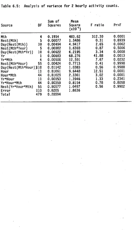
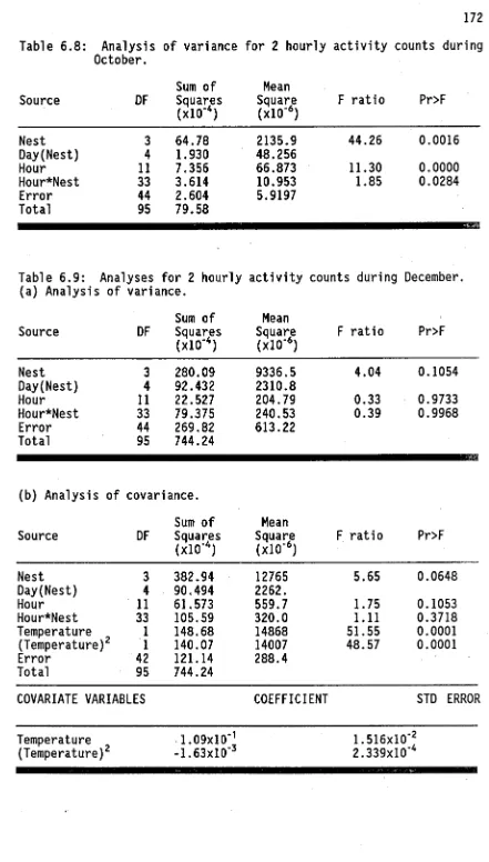
(19) xvii. LIST OF TABLES. 3.1. Analysis of variance for nearest neighbour distances of trees 40 always, sometimes, and never occupied by ants. 4.1. Numbers of colony founding queens reared at various temperatures from 1986 to 1989.. 49. 4.2. Numbers of queens in colony founding nests.. 65. 5.1. Analysis of covariance for proportions of larvae in nests. 106 5.2. Analysis of covariance for proportions of pupae in nests.. 106. 5.3. Analysis of covariance for ratios of major worker to minor worker adults in nests.. 106. 6.1. Numbers of days per month of successfully completed activity 142 trials from November 1986 to March 1989. 6.2. Analysis of variance design for total day activity counts. 144 6.3. Analysis of variance design for 2 hourly activity counts on individual nests within each month.. 145. 6.4. Analyses of covariance for daily activity.. 163. 6.5. Analysis of variance for 2 hourly activity.. 165. 6.6. Analysis of variance for 2 hourly activity during May.. 169. 6.7. Analyses of variance and covariance for 2 hourly activity during August.. 169. 6.8. Analysis of variance for 2 hourly activity during October.. 172. 6.9. Analysis of variance and covariance for 2 hourly activity during December.. 172. 6.10. Analysis of variance and covariance for 2 hourly activity during January.. 175. 6.11. Analysis of variance and covariance for 2 hourly activity during March.. 179. 6.12. Seasonal and circadian patterns of activity in nests.. 182. 6.13. Frequencies of prey items collected by foragers.. 189. 6.14. Analyses of variance for daily prey intake measures.. 193. 6.15. Analyses of variance for circadian patterns in prey intake.196 6.16. Analysis of variance for scape lengths of ants.. 199.

(20) 6.17. Analysis of covariance for weights of foragers and nest ants.. 199. 6.18. Analysis of covariance for daily weight difference between leaving and returning ants.. 203. 6.19. Analysis of covariance for circadian patterns in weight difference between leaving and returning ants.. 203. 6.20. Analysis of variance for circadian patterns in weights of ants leaving the nest.. 209. 7.1. Frequencies of arthropods found in leaf samples.. 236. 7.2. Analysis of variance for numbers of. 236. Coccus sp.. 7.3. Analysis of variance for numbers of ant-tended homoptera.. 238. 7.4. Analysis of variance for numbers of. 238. Phenacaspis dilata.. 7.5. Analysis of variance for numbers of spiders.. 241. 7.6. Analysis of variance for numbers of Coleoptera.. 241. 7.7. Analysis of variance for numbers of Diptera.. 242. 7.8. Analysis of variance for numbers of Psocoptera. 242. 7.9. Analysis of variance for numbers of non-tended arthropods. 243 7.10. Analysis of variance for numbers of eggs.. 243. 7.11. Analysis of variance for proportions of homopteran-scarred leaves.. 247. 7.12. Analysis of variance for proportions of eaten leaves.. 247. 7.13. Analysis of variance for proportions of undamaged leaves. 251 7.14. Analysis of variance for proportions of both homopteran-scarred and eaten leaves.. 251. 7.15. Analyses of variance and covariance for area of leaf eaten.254 7.16. Analyses of variance for numberi of spikes per m 3 in July 1987.. 256. 7.17. Analyses of variance for numbers of spikes and fruit per m 3 in October 1987. 258 7.18. Analysis of variance for number of fruit per tree sector in November 1987.. 259.

(21) 1.. General introduction.. The weaver ants of the genus. Oecophylla are prominent members of. forest insect communities throughout all of the tropical world except America. The two extant species are quite similar in morphology and behaviour, but display some colour variation.. O. smaragdina (Fab.). ranges from tropical Asia to northern Australia, and onto some western Pacific islands (fig 3 ..1). The Australian subspecies,. virescens (Fab.),. has a pale green abdomen, hence the common name of green tree. ant. (Dodd, 1928), while mainland Asian populations have a uniform reddish brown colour (Wheeler, 1922). The African species,. 0. longinoda. (Latr.), varies from reddish brown to dark brown.. 1.1. Nest structure.. The weaver ants' most distinctive feature is their habit of using silk produced by their larvae to construct nests of living leaves. This process was described independently by Ridley (1890, in Wheeler, 1910) in India and Saville-Kent (1891, in Hemmingsen, 1973) in Australia. Further accounts have been given by Doflein (1905), Ledoux (1950), Hemmingsen (1973), and Holldobler and Wilson (1983b). The following description is derived primarily from the 2 most recent sources. When a new nest is required, individual workers scout for suitable clusters of leaves, which they grab with their mandibles and attempt to draw together. Other workers are attracted to the site, presumably by the success of the first workers, and join the effort. A large gap can be bridged by chains of ants, formed by each ant clasping the.

(22) 2 petiole of the ant in front with her mandibles. Chains of at least 10 ants, spanning over 5 cm in length can be constructed; this chaining appears to be unique- to the weaver ant genus. Eventually, a number of leaves will have been stretched into position for binding, each held in place by rows of workers. Other workers carry late instar larvae in their mandibles to the binding sites. With a precise, coordinated set of movements, the ant uses the larva to lay a series of silken strands between the leaf margins, until a white sheet of silk joins the two. The larva moves very little during this "weaving" operation, acting as a passive shuttle. Accounts of the variation in nest weaving with time of day, and with worker castes involved, have shown some discrepancies. Hemmingsen (1973) in Thailand observed nocturnal weaving with larvae by the larger major caste adults on the outside of the nest, while the smaller minor workers wove inside the nest during the day. Some earlier workers also suggested that little weaving occurred during the day, but. Ledoux. (1950) and H011dobler and Wilson (1983b) both recorded daytime weaving on the outside of the nest. Diurnal weaving behaviour may vary among different populations, or possibly environmental factors such. as. temperature and relative humidity influence the times when larvae are used for weaving. Less complex forms of nest weaving occur in 3 other genera of the subfamily Formicinae. Both species of the genus. Dendromyrmex. (Wilson,. 1981) incorporate larval silk into their nests, which are also bound with fungus-impregnated vegetable fibre (or "carton"). Larvae perform all of the weaving movements to lay silk onto the nest, while being held passively in an appropriate site by adult worker ants, and will add silk to the nest even when unattended by workers. At least. 2.

(23) 3 species in the genus species of. Camponotus (Schremmer, 1979), and a number of. Polyrhachis (Holldobler and Wilson, 1973b) also use larval. silk in nest construction. In the few species observed to date, all larvae were held to stimulate silk production, but the larvae performed most of the weaving motions. Holldobler and Wilson (1983b) have fitted these examples to an evolutionary gradient, from the primitive weaving of. Dendromyrmex to the complex, highly coordinated nest construction. in. Oecophylla. The nests of some Cuban species of. Leptothorax, and Technomyrmex. bicolor textor, from Java, also contain silk, but no evidence for larval production of this silk has been observed. As these species belong to the subfamilies Myrmicinae, and Dolichoderinae, respectively, which have no other weaving species, this silk is probably from other sources, such as spiders' webs. The size of. Oecophylla nests vary from a single folded leaf to. many hundreds of leaves (plate 1.1). These size differences are controlled to some extent by the structure and density of foliage.. A. single palm frond, for example, can be utilized as a nest by joining the two sides of the frond with silk (Way, 1954a). Occasionally, ants construct nests in plants with very small leaves, such as. Leptospermum. species; such nests have walls composed almost entirely of silk (plate 1.1c). Nevertheless, some plants appear to be generally unsuitable for nest construction. The large leaves of plantain, the narrow leaves of oil palm, and the small leathery leaves of cashew, for example, were not utilized for nesting by the African weaver ant (Taylor, 1977)..

(24) 4. Plate 1. Leaf nest of 0. smaragdina. nest built from 1 leaf of Elaeodendron melanocarpum. Multiple leaf nest in Drypetes lasiogyna. Nest in Leptospermum sp. Nest in Pongamia pinnata (still occupied although all leaves were dead).

(25) 4a. Plate 1..

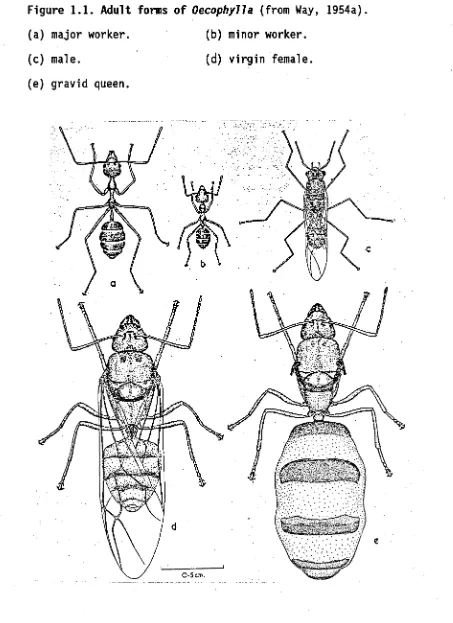
(26) 5 1.2 Colony structure.. Weaver ants are predominantly arboreal (e.g. Holldobler, 1980; Way, 1954a), but sometimes venture onto the ground to forage, or travel between trees when canopies do not interconnect (Jackson, 1988; Taylor and Adedoyin, 1978). Their colonies are among the largest in the ant family. Way (1954a) observed one colony inhabiting 151 nests, scattered throughout 8 coconut and 4 clove trees, and covering an area of 800 m2 He estimated that this colony contained 480,000 worker ants,. and. 280,000 brood. Vanderplank (1960) and Holldobler and Wilson (1978) also report populations of mature colonies in the range of 100,000 to 500,000, and Leston (in Majer, 1976a) estimated that colonies could number several million. Most polydomous ant species (i.e. species whose colonies comprise more than one nest) have more than one reproductively active queen. However, a mature Oecophylla colony is strictly monogynous; the loss of the single gravid queen signals the demise of the entire colony (Crozier, 1970; Greenslade, 1971b; Holldobler and Wilson, 1977b, 1983a; Way, 1954a). Greenslade (1971a) estimated from cyclical patterns. of. abundance in Solomon Island plantations that the average life span of colonies was 8 years. Vanderplank (1960) successfully reared colonies in potted clove plants for 5 years. The various adult forms of weaver ant are shown in figure 1.1. The worker population is polymorphic (Cole and Jones, 1948; Weber, 1949). The smaller minor caste workers tend the brood, and rarely venture outside the nest. The larger major caste workers forage, and assist with care of the queen and larger brood. The major workers also defend the colony territory, although both castes will act in nest defence.

(27) Figure 1.1. Adult forms of Oecophylla (from Way, 1954a). (a) major worker.. (b) minor worker.. (c) male.. (d) virgin female.. (e) gravid queen..

(28) 7 (H011dobler and Wilson, 1977b). A feature unique to the weaver ant genus is that major workers outnumber minor workers (Wilson, 1953). Winged male and female sexuals are produced during the wet season, and are released after rain (Bhattacharya, 1943; Gibbs and Leston, 1970; Greenslade, 1971b; Way, 1954b). Inseminated queens select a suitable site within a curled leaf or a cluster of leaves, and rear their first brood claustrally. Both haplometrotic colony founding (by a single queen - Dodd, 1902, 1928; Greenslade, 1972; Vanderplank, 1960) and pleometrotic colony founding (by a group of queens - Begg, 1977; Ledoux, 1950; Peeters and Anderson, 1989; Richards, 1969) have been recorded. Weaver ants maintain their territory and coordinate their activities using a highly developed chemical communication system, in combination with visual and tactile cues. Ants are recruited to food, unexplored terrain, and territorial intruders using odour trails released from the sternal and rectal glands in the abdomen (Holldobler and Wilson, 1978). Well established trails between nests are. marked. with rectal gland secretions, which remain effective for about three days (Jander and Jander, 1979). Localised alarm and attack responses are invoked by volatile chemicals from the mandibular gland. in the. head, and poison and Dufour's glands in the abdomen (Bradshaw, Baker, and Howse, 1975, 1979a,b,c). Drops of faecal material are deposited randomly throughout the colony territory; workers can distinguish alien from friendly terrain using these territorial marks (H011dobler and Wilson,. .. 1978, 1977a). This sophisticated chemical communication. repertoire is among the most complex observed in the ant family. The combination of well developed communication, aggressive territoriality, and decentralized multiple nests allows Oecophylla to.

(29) 8 maintain absolute territories, which exclude most other ant species (H011dobler and Lumsden, 1980). Similar absolute territories have been reported in a number of polydomous tropical ants with large populations (e.g. Greenslade, 1971b; Leston, 1970, 1973, 1978; Majer, 1972; Room, 1971). The patchwork distribution of the exclusive territories of weaver ant and other dominant arboreal ant colonies has been termed the ant mosaic by Leston (1973). Interestingly, a few ant species can coexist with. Oecophylla,. without invoking a massive defence response (Holldobler, 1980, 1983; Room, 1971). This selective enemy specification has also been observed in. Pheidole dentata, and allows defensive responses to be directed. towards the most serious competitors for essential resources, such as food and nest sites (Wilson, 1975, 1976c). In tropical arboreal mosaics, absolute territories appear to have evolved in response to competition for foraging space, rather than nest sites (Leston, 1973; Majer, 1976a,b; Room, 1971).. Oecophylla and other dominant ants act as keystone species (Paine, 1974, 1976), exerting a strong controlling influence on the other arboreal insect fauna through predation and competition for food resources (e.g. Bigger, 1981; Majer, 1976c; Risch and Carroll, 1982a,b; Way, 1954a). Before examining this aspect further, the diet of weaver ants will be described.. 1.3. Diet.. The weaver ant, like many ant species, collects two food types: honeydew from various homopterans (and lycaenid caterpillars), and insect prey (Carroll and Janzen, 1973). Honeydew is collected from many.

(30) 9 families of homoptera, including Coccidae, Stictococcidae, Pseudococcidae, Aphididae, Margarodidae, Membracidae, and Cicadellidae (Brown, 1959; Das, 1959; Vanderplank, 1960; Way, 1954a, 1963). Many ant-homopteran interactions are mutually beneficial; the ants obtain food rich in sugars and amino acids, and the bugs obtain some protection from predators and parasites (Way, 1963). The coccid,. Saissetia zanzibarensis, has developed a strongly. mutualistic association with the African weaver ant (Way, 1954b). Without ant attendance, the coccids are virtually exterminated by contamination with mould, parasitism, and predation.. 0. longinoda. workers also transport coccid nymphs to optimum feeding sites, and "cull" excess numbers by consuming them. A number of lycaenid butterfly larvae (which produce sugary secretions from specialized dorsal glands) are also tended by ants, and are often kept within small leaf nests. Lycaenids tended by green tree ants in Australia include. Anthene se7tuttus, Arhopala centaurus,. Arhopala micale, Hypolycaena phorbas,. and. Theclinesthes miskinf. eucalypti (Common and Waterhouse, 1981). However, this source of food is generally much less important than homopteran honeydew. Weaver ants are generalist predators, attacking most arthropods that they encounter. The most abundant prey items recorded by Vanderplank (1960) were termites, ants, and honeybees. Other prey carried back to the nest include heteropterans, coleopterans, orthopterans, blattodeans, mantodeans, djpterans, and araneans (Majer, 1976c; Vanderplank, 1960; Way, 1954a).. Oecophylla can reduce the levels. of many untended insect groups substantially (Leston, 1973; Majer, 1976c; Room, 1973). For this reason, various studies have examined the potential of these ants to control certain insect pests of tree crops..

(31) 10. 1.4 Impact of weaver ants on arboreal arthropod pests.. The earliest known example of biological control, recorded in the Nan Fang Ts'ao Mu Chuang (about 340 AD), described how. 0. smaragdina. was used to control insect pests in Chinese orange orchards. Groff and Howard (1925) reported that citrus growers in the Saisha district import nests of weaver ants from southern China to protect their crops from the heteropteran,. Tesseratoma papillosa, and some boring insects.. However, weaver ants also increase the numbers of the harmful red scale,. Aonidiela aurantii, in citrus trees, presumably by excluding. its parasites (Flanders, 1958). In Zanzibar,. 0. longinoda improves coconut crop yields by reducing. the levels of the coreid bug,. Pseudotheraptus wayi, which causes. premature nutfall (Vanderplank, 1960; Way, 1953, 1954a). Similarly,. 0.. smaragdina protects coconuts in the Solomon Islands from another coreid,. Amblypelta cocophaga (Brown, 1959; Greenslade, 1971a; Stapley,. 1971). In cocoa trees, weaver ants reduce damage from the capsids,. Distantiella theobroma and SaMbergella singularis (Dun, 1954; Leston, 1970, 1973; Majer, 1976c). They also tend various stictococcids, but discourage the pseudococcid,. Pseudococcus njalensis, which transmits. swollen shoot virus (SSV). Ants of the genus. Crematogaster tend P.. njalensis, and thus aid the spread of the virus (Leston, 1970; Strickland, 1951). One pseudococcid tending species,. C. castanea, can. coexist with weaver ants, but the effect of this association on virus transmission has not been determined (RoOm, 1971; Taylor, 1977). Other documented impacts of fruit from. Oecophylla include protection of mango. Cryptorrhynchus weevils (Friedrichs, 1920); reduction of.

(32) 11 most insect pests in tea seed trees, but an increase in tended coccids (Das, 1959); and in arabica coffee, protection from the pentatomid,. Antestiopsis intricata, but increased damage from homopterans (Das, 1959; Leston, 1973). Leston (1973) and Room (1973) have outlined strategies for the development of insect pest control by manipulation of the ant fauna. Stapley (1971) successfully encouraged the spread of weaver ants in Solomon Island coconut plantations by exterminating the nests of its major competitor,. Pheidole megacephala, with selective insecticide and. herbicide treatments. Many ant manipulation trials have failed, however, due to lack of biological and ecological knowledge of the species concerned. Transplantation of weaver ant nests, for example, rarely leads to successful colony establishment because the reproductively active queen is not collected (e.g. Brown, 1959). A colony fragment also has little chance of surviving within the territories of other dominant ant species in the mosaic (Leston, 1973). The usefulness of an ant species in crop protection may be nullified by detrimental interactions with other insect fauna. As already mentioned, ants can increase the levels of tended homopterans to harmful levels, and coexisting ant species may encourage detrimental insect species. By reducing predator populations, ants may allow some herbivores which are less vulnerable to ant predation, such as leafminers, to increase to harmful levels (Fowler and MacGarvin, 1985; Fritz, 1983). The effectiveness of ant control may also vary temporally. For example, seasonal changes in the protein requirements of the colony, caused by seasonal patterns of reproduction (e.g. Brian. et al, 1981;. Sudd, 1987), can also alter the level of predation on insect pests.

(33) 12 (e.g. Greenslade, 1971b; Robertson, 1988; Skinner, 1980b).. 1.5 Aims of the present project.. Almost all previous work on the weaver ant genus has been conducted in the relatively non-seasonal environment of the wet tropics. The present study was undertaken to examine the distribution, colony structure, and activity of the green tree ant, 0. smaragdina, and its impact on the arboreal arthropod fauna, in the highly seasonal, dry tropical environments which characterize most of northern Australia. The study aimed to answer the following questions: What limits the distribution of green tree ants within Australia (chapter 3)? Is there seasonal and geographic variation in the reproductive activity of colonies (chapter 5)? If so, are these related to physical environmental factors such as temperature and rainfall (chapter 4+5)? Does the structure and extent of colonies change seasonally, in response to reproductive cycles and/or environmental factors (chapter 5)? Does the behaviour and activity of ants vary seasonally and in response to environmental conditions (chapter 6)? More detailed analysis of activity dynamics (e.g. circadian task switching, length of foraging trips) was inhibited by the extreme aversion of these ants to any form of tag. Do green tree ants have a significant impact on other arthropod populations, or on the condition of their host trees, in this environment (chapter 6+7)?.

(34) 13. 2. Description Of Study Sites. 2.1. Townsville.. Townsville (19°16'S, 146°48'E) lies on the edge of a narrow coastal plain in north-eastern Queensland (figure 2.1), bordered to the west by the Hervey's Range/Paluma Range escarpment, and to the east by the Coral Sea. Although this area originated as part of the Tasman geosyncline in the lower Paleozoic (500 - 600 million years ago), no rock formations from the early periods of this era occur on the land surface (Henderson, 1980). The earliest outcroppings in the region are the western escarpment, and residual mountains and hills, probably produced by granitic intrusions emplaced during the Devonian to Permian periods (280 to 400 million years ago), and raised into their present positions in the late Tertiary period to the early Quaternary period (10 to 30 million years; Hopley, 1978). This uplifting has produced the present system of relatively short streams (e.g. Ross River, Bohle River) flowing eastward from the escarpment and residuals into the sea, and streams to the west of the scarp (e.g. Keelbottom Creek, Star River) draining into the Bu'rdekin River. Examples of the residual granitoid mountains in the Townsville region include Mount Stuart, Castle Hill, and the Mount Elliot Range. The coastal lowland consists of alluvia eroded from the uplifted escarpment and residuals during the Quaternary period. Climatic fluctuations during glacial -interglacial cycles produced varying levels of deposition, and weathering of sediments. Recently, an increase in sea level has caused a small rise in rainfall, and thus deposition, although still high, has probably decreased slightly (Hopley, 1978)..

(35) 14 Figure 2.1. Map of northern Queensland showing locations of study sites.. 145'E. 15°S. Cairns. Townsville Major Creek •. Bowen. Proserpine • Mackay •. Yeppoon.

(36) 15 Most of these lowlands have mature, solodic, solodized soils, with well developed horizons (Murtha, 1978). The presence of a heavy clay horizon beneath shallow (15 - 25 cm) topsoil impedes' drainage, and limits the agricultural potential of the area. The best soils in the region are associated with recent alluvial deposition, along flood plains, and old stream beds, and on the fringes of mountains and the coast. Rainfall in the Townsville region is highly seasonal, with an average of 80% of the 1200 millimetre mean annual precipitation falling during the summer months from December to March (Bureau of Meteorology, 1975). These summer rains are occasionally generated by a widespread monsoonal trough, but more often by the irregular passage of upper atmospheric troughs or cyclones (Oliver, 1978). The time of onset, duration, and intensity of the wet season, and the annual precipitation level can thus fluctuate widely from year to year. Monthly rainfall figures recorded in Townsville from 1985 to 1989 (figure 2.2a) clearly demonstrate these trends. Wet season rainfall levels ranged from 257 mm (in 1984/85), to 1014 mm (1988/89), the commencement of the wet varied from October (1985/86) to February (1984/85), and the duration of the wet from 2 (1984/85) to 5 months (1988/89). Temperature ranges from a mean maximum of 30.7°C in January, to 24.4°C in July, and mean minimum temperature from 24.5°C in January, to 15.4°C in July (Bureau of Meteorology, 1975). Frosts are very rarely experienced in this coastal region (Foley, 1945), with none recorded during the course of my project. Temperature undergoes much more consistent seasonal variation than rainfall, with mean monthly maximum and minimum temperatures during 1985 to 1989 differing by only 2.3°C and 5.7°C, respectively, from year to year (figure 2.2b)..

(37) 16 Figure 2.2. Climatic patterns in Townsville from January 1985 to May 1989.. Figure 2.2a. Rainfall patterns Rainfall(mm) 300 250 200 150 100 60 -. 11111111"1 Ill'T11111. 0 1. 1 3 5 7 9 85. 3 5 7 9 11 86 1. 1. II I dal. 3 5 7 9 11 1 87. 3 5 7 9 111 3 88 1 89. I. Date. Figure 2.2b. Temperature patterns 35. Temperature (°C). 30. 25. 20. 15. 10. '1'1'1'1'1'1'1'1 '1' 1'1'1'1''1'1'''1'1'1'1'1'1' 1 3 5 7 9 11 1 3 5 7 9 11 1 3 5 7 9 11 1 3 5 7 9 11 1 3 5 85 1 86 87 1 1 89 1 1 88 Date.

(38) 17 Based on these climatic figures, the Holdridge (Holdridge. et al, 1971). life zone classification system places Townsville within the cooler portion of the tropical dry forest zone. The combination of poor soils and relatively dry, seasonal climate has constrained vegetation development in the region to open eucalypt woodland (plate 2.1), dominated by narrow-leaved ironbarks. (E.. drepanophylla), poplar gums (E. platyphylla), and the introduced chinese apple. (Zizyphusmauritiana). Cockatoo apple (Planchonia careya). and broad-leaved paperbark. (Melaleuca viridiflora). understorey trees, and spear grass. are common. (Heteropogon spp.), kangaroo grass. (Themeda australis), and the naturalised red natal grass (Rhynchelytrum repens) the main grasses. In regions of better soil quality, more complex and dense vegetation has developed, with occasional patches of quite dense closed forest. My Townsville study site was located within one such area, bordering Campus Creek, adjacent to the James Cook University campus (plate 2.2). All trees over 2 metres tall in the site were mapped using a bearing compass, tape measure, and an optical distance gauge, in 1985 (figure 2.3). This map was updated as trees grew, or died. The area to the east of the creek was open eucalypt woodland, which was uninhabited by green tree ants, and therefore unmapped. In May, 1988, 744 trees were found in the 14106 m2 site, giving a density of 0.053 trees per m2. .. The commonest tree species were chinese apple. (Zizyphus. mauritiana), northern swamp box (Lophostemon grandiflorus), Pongamia pinnata, and Melaleuca spp., but many other species were also present (listed in figure 2.3). Vines were also abundant, including native jasmine. (Jasminium didymum subsp. racemosum), stinking passion flower. (Passiflora foetida), native grape (mainly Cayratia trifolia),.

(39) 18 Plate 2.1. Open eucalypt woodland of the Townsville region..

(40) 19 Plate 2.2. Vegetation of the Townsville study site. (a) Campus Creek in January 1989. (b) Campus Creek in October 1987. (c) Transitional zone from riparian forest to open woodland,.

(41) 20 Plate 2.3. The Major Creek mango plantation. Plate 2.4. Sampling the upper canopy of mango trees..

(42) Legend for tree species found in Townsville study site.. A. 0 A. 'r p. F. Zizyphus mauritiana Lophostemon grandiflorus Pongamia pinnata Eucalyptus platyphylla Eucalyptus tessellaris Eucalyptus papuana Canarium australianum Pleiogynium timorense Melaleuca spp. Elaeodendron melanocarpum Drypetes lasiogyna Pouteria sericea Exocarpos latifolius Acacia salicina Lysiphyllum hookeri Planchonia careya Alphitonia excelsa Gardenia ochreata Ficus opposita Cochlospermum gillivraei.

(43) 21 Figure 2.3. Map of Townsville study site showing colony, extents in May 1988..

(44) 22 and the introduced rubber vine. (Cryptostegia grandiflora). Where tree. cover was sparse enough to allow sufficient light through, an extensive ground cover was present, with herbs such as. jamaicensis,. the introduced. Stachytarpheta. Lantana camara, Hyptis suaveolens,. Crotalaria spp., and Triumfetta rhomboidea. These herbaceous shrubs were interspersed with clumps of grass, mainly spear grass, kangaroo grass, red natal grass, and guinea grass. (Panicum maximum).. Plant species were identified by Dr. B.R. Jackes, Botany Department, James Cook University, or using the keys in her recent monograph, "Plants of Magnetic Island" (1987). The vegetation of this site was markedly seasonal, due to the strong seasonality of rainfall. Some of the trees in the site, such as. Pongamia pinnata, Zizyphus mauritiana, and Eucalyptus platyphylla. were. deciduous to varying degrees. This was particularly evident in late 1987 (plate 2.2b), after a very poor wet season (figure 2.2a). Most herbs and grasses also dwindled or disappeared during the dryer months, producing a much more open understorey later in the year. Insect numbers also varied seasonally, peaking in the wet season when foliage was abundant. Although not assessed in the present study, this trend has been well documented for tropical habitats in Costa Rica (Janzen and Schoener, 1968) and Ghana (Gibbs and Leston, 1970; Leston,. 1970).. The most conspicuous arboreal ant species was the green tree ant,. Oecophylla smaragdina. Other ants observed in trees included species of. Crematogaster, Iridomyrmex, and Polyrhachis, Opisthopsis haddoni,. Paratrechina longicornis, and Tetramorium bicarinatum. The commonest nocturnally active arboreal ants were. 0. smaragdina and several. Camponotus species. In more open areas, the meat ant,. Iridomyrmex purpureus sanguinea.

(45) 23 predominated. This dolichoderine ant was the only species which engaged in major conflicts with the green tree ant. Less conspicuous grounddwelling ants included other species of Iridomyrmex, Camponotus spp,. Odontomachus sp, and Cerapachys sp. Ant species were identified by Dr. R.W. Taylor, Australian National Insect Collection, CSIRO Division of Entomology, Canberra. No voucher specimens have been lodged outside James Cook University. to. date.. 2.2 Major Creek.. A second study site was established in 1986 on a plantation of mango trees (Mangifera indica) owned by the Wright family, about 1 km from Major Creek in the foothills of Mt. Elliot Range (plate 2.3). Mangos were the only fruit tree crop grown in this region of Queensland on a scale sufficient to support adequate populations of green tree ants for my research. The Major Creek farm was chosen because the owner was the sole person in the district who did not regularly use insecticidal sprays (which are very effective at destroying ants). Major Creek is approximately 50 km from my Townsville site,. and. experiences a relatively similar climate (K. Wright, pers. comm.; Oliver, 1978). Two fields of trees were mapped, totalling 250 trees (figure 2.4). The 120 trees in field A were planted in 1974, and the 130 field B trees in 1976. As the average tree height was only 6.5 metres, access to all parts of the canopy was relatively easy, by ladder (plate 2.4), or by climbing. Trees were arranged in a square grid pattern, with an average spacing of 9 metres. No canopy interconnections between trees.

(46) 24 had developed, due to the you. density of trees.. Regular slashing confinec. vegetation to grasses, small. herbs such as Stachytarpheta. and coppice regrowths of. Zizyphus mauritiana.. The ant. ;Major Creek plantation had. a similar species composition. ille site. However, ground-. oh: -. dwelling ants were more. arboreal ants fewer, as. vegetation levels were lower. abitat.. Figure 2.4. Map of Major Creek. luring May 1988.. - Mango tree unoccupi. - Mango tree occupied. tree ants. '2e ants.. Field. 0 0 0 0 0 0 0. 0. ,7). 0. -;.;. 0. 0. 0. 0. 0. • • • 0 0 0 • • 0. 0 0 0 0. 0 0 0 0. 0 0 0 0. 0 0 0 0. 0 0 0 0 0 0. 0. 0. 0. 0. 0. 0. 0. 0. 0. 0. 0. 0. 0. 0 0. 0. Field 0. 0 0. 0 0. 0. 0. 0. 0 0 0 0 0 0 0 0 0. 0. 0 0. 0 0. 0. 0. 0. 0. 0. 0 0 0 0. •. 0. 0. 0 0 0 0 0 0. 0 0. 0. 0. 0. 0 0 0 0. 0. 0. 0. 0-0 0 0. 0 0 0 0. -!) 0. ) ) •• ) • •. 0 0 0. 0 0 0 0. 0 0. 0 0 0. 0. 0. 0. 0.

(47) 25. 3.. Distributional patterns.. 3.1. Introduction.. The weaver ant genus, Oecophylla, occurs throughout much of the forests of the old world tropics (figure 3.1). The African weaver ant,. 0. longinoda, inhabits tropical Africa (Ledoux, 1950; Way, 1954a; Wheeler, 1922). The only other extant species, 0. smaragdina, ranges from India, across most of tropical Asia to northern Australia, and onto many tropical western Pacific islands, as far east as Fiji (Cole and Jones, 1948; Dodd, 1928; Groff and Howard, 1925). The genus is absent from the tropical forests of America, which have an otherwise very diverse arboreal ant fauna (Wilson, 1959). Wheeler (1922) further subdivided the 2 species into various subspecies and varieties, based on their considerable geographic variation. These morphological differences, and discrepancies in genetic studies by different workers (Bhattacharya, 1943; Ledoux, 1950; Vanderplank, 1960; Way, 1954a) have led Crozier (1970) to suggest that more than 2 species may exist. No-one has yet conducted a comprehensive genetic study to examine this possibility. A number of extinct species have been identified from European tertiary fossil deposits (figure 3.1). Fifty specimens of 0. brischkei Mayr, and one specimen of 0. brevinoda Wheeler were found in Baltic amber from the early Oligocene epoch, 30 to 34 million years ago (Wheeler, 1914). These fossils are among the oldest records of ant genera still surviving today. Fossil remains of 24 extant genera have been identified from Oligocene sediments, and only one extant genus.

(48) 26. Figure 3.1. World distribution of weaver ants.. Oecophylla smaragdina. Oecophylla longinoda. Fossil records of. Oecophylla. 4t,* ,Ioi I,. , iitp ...,-p. ,. .. *AIII0 1. •. /41 /4 IIIII. .. 1. CI 4. q. p. fr)1.. O. O CO. O. O. O. O CD.

(49) 27. (Iridomyrmex) from an earlier Eocene deposit (Wilson, 1987). Another species,. 0. sicula, has been described from upper Miocene amber. deposits in Sicily (12 to 15 million years ago). These species can be placed in a morphocline, consistent with the geological sequence, from. brevinoda - brischkei - sicula - present species. A lower Miocene deposit, recently discovered by L. Leaky, on Mfwangano Island, Kenya, contained over 300 specimens of Oecophylla. leakeyi Wilson and Taylor, which most closely resembles O. brischkei in morphology. This unique fossil assemblage is probably the remains of an arboreal leaf nest, very similar to those constructed by present day weaver ants (Wilson and Taylor, 1964). Other common features include naked pupae (with no silk cocoon), and an adult size frequency distribution unique to this genus (with the larger major caste. more. numerous than the smaller minor caste). These findings suggest that the genus Oecophylla has remained remarkably stable in morphology and social structure for at least 20 million years. Weaver ants disappeared from the Mediterranean area as it drifted out of the tropics with the northward migration of the Eurasian and African continental plates, producing a cooler climate (and associated vegetation changes). No Oecophylla fossil records have been discovered in the Australian region, so no information on the separation of the 2 present species and their biogeographical history is available. spread of the ancestral. The. O. smaragdina into Australia was unlikely to. have occurred more than 15 to 20 million years ago, when this continent was significantly further south , and first collided with the Asian continental plate (Henderson, 1980). In recent times, the distribution of the green tree ant in Australia has probably fluctuated, increasing during interglacials when.

(50) 28. temperatures and rainfall were higher and lowland closed forests expanded, and shrinking during glacial periods (Kershaw, 1978). A major reduction in forests between 40000 and 30000 years ago, which Singh. et. al (1981) suggest was caused by a combination of decreased rainfall and aboriginal use of fire, reduced the available habitat for this ant species. A subsequent increase in rainfall and temperature after the end of the last glacial 10000 years ago has allowed the closed forests, and thus the range of the green tree ant, to re-expand. The earliest European observation of the green tree ant was made by Joseph Banks, when James Cook first sailed along the east coast of Australia in 1778. He recorded this species as far south as Bustard Bay (24°S). The present distributional limits of. Oecophylla have not been. examined in Australia, or elsewhere in the world. The large arboreal nests and aggressive nature of these ants make them highly conspicuous, and readily observed if present, so they make ideal subjects. for. distributional studies.. 3.2. Methods.. Questionnaires were sent to all local government offices in Australia north of latitude 30°S, asking whether. 0. smaragdina was. present in their shire. Because these ants are conspicuous, and are considered a nuisance by many householders (due to their bite), it is unlikely that people would be unaware of their presence if populations existed. Twenty of the 22 offices contacted answered the questionnaire. This survey was 'supplemented by the direct inspection of 24.

(51) 29 localities in coastal northern Queensland, between latitudes 15° and 30°S, during 1985. These sites were chosen primarily as accurate climatic data were available from the Bureau of Meteorology (1975, Foley, 1945), and also to cover the widest possible geographic range. The effectiveness of various weather parameters in predicting the distribution of. 0. smaragdina within Australia was tested using. discriminant analyses. Micro-distributional patterns were monitored in my Townsville study site, in conjunction with colony size observations (section 5.3.1). Each of the 750 trees in the site was surveyed for the presence of ants, in the following sequence. Firstly, the trunk and lower branches of the tree were examined for ant trails. If no ants were found, binoculars were used to scan the canopy for trails and nests. The presence of nests alone was never accepted as proof of ant presence, as nests were often abandoned in seemingly healthy condition during colony contraction periods. Some large trees had dense foliage that obstructed observation; for these, I climbed into the canopy to look for ants. Using this combination of techniques, quite small pOpulations could be detected. Surveys were conducted twice yearly from 1986 to mid 1987, and every two months from July, 1987 till May, 1989. .. The effect of tree density on distribution patterns was tested using a nearest neighbour technique (Greig-Smith, 1983). Trees were divided into three groups: trees which were occupied by ants on every survey, trees inhabited at least once during the study, and trees never occupied by ants. The distances from 60 randomly chosen trees within these categories to their nearest neighbours were measured, and compared using an analysis of variance. Preferences for particular tree species were examined by comparing the proportions of the total trees.

(52) 30 of each species always, sometimes, and never occupied, for the most common species. The interactive effect of these two variables on nearest neighbour distances was examined using a 2 way analysis of variance.. 3.3. Results. 3.3.1. Distribution in Australia.. The presence and absence of 0. smaragdina in 46 sites across northern Australia was mapped in figure 3.2. No colonies were recorded south of the tropics, with Broome, W.A. (17°57'S) the southern limit of distribution on the west coast, and Yeppoon, Qld (23°6'S) the southern limit on the east coast. Distribution in Queensland south of latitude 15°S was restricted to the coastal plain by the Great Dividing Range. The highest elevation where this ant was observed was 500 metres above sea level, west of Cairns (16°50'S). Isotherms and isohyets are shown on figure 3.2, but neither corresponds closely to the distribution of Oecophylla. The 17°C mean minimum temperature isotherm demarcated the distributional limits of this ant species reasonably well in eastern Australia, but extended too far south in western Australia. Similarly, the 500 mm average annual rainfall isohyet successfully separated sites with and without green tree ants in the west, but not in the east. Nor did any single temperature statistic (average, mean minimum, mean maximum annual temperature; number of frost days per annum) or rainfall variable (annual rainfall, number of rain days per year) appear to explain the.

(53) 31 Figure 3.2. Australian distribution of 0. smaragdina. • Sites with. o. 0. smaragdina.. Sites without. 0. smaragdina.. 500 and 750 mm mean annual rainfall isohyets and 17°C average minimum temperature isotherm are shown.. 20'S. 17°. 10'S.

(54) 32 observed distribution pattern. When the data were plotted against rainfall and temperature in combination (figure 3.3a), much better separation between sites with and without ants was observed, with a curvilinear line of demarcation. To linearize this boundary, temperature and rainfall figures were converted to logarithms (figure 3.3b). To determine which combination of climate parameters could best predict the observed distribution pattern, linear discriminant analyses were performed on various combinations of the transformed temperature and rainfall data. Mean minimum temperature (Li n ) and average annual rainfall (R) were the most successful variables, correctly classifying 98% of the sites (Lokkers, 1986). The line of demarcation calculated by the discriminant analysis was:. 4.26 log(R) + 23.5 log(Tmin ) - 42.4 = 0. This analysis demonstrates that a combination of high temperature and high rainfall was necessary to support populations of. 0. smaragdina.. The curvilinearity of the boundary further suggests that either variable in isolation could limit distribution of this species at its lower extremes. Some data published by Way (1954b) on the distribution of. 0.. longinoda in eastern Africa was also entered onto the discriminant plot. All 6 sites (3 with and 3 without ants) were classified correctly by the discriminant function calculated for the Australian species..

(55) 33 Figure 3.3. Temperature and rainfall averages of sites with and without 0. smaragdina. Townsille marked with asterisk.. Data for 0. longinoda from African study by Way (1954b). + Sites with 0. smaragdina.. ❑ Sites without 0. smaragdina.. A Sites with 0. longinoda.. v Sites without 0. longinoda.. Figure 3.3a. Linear scales on axes Rainfall (mm). 1500. 1000. 500. 0 13. 15. 17. 19. 21. 23. Temperature ( eC). Figure 3.3b. Logarithmic scales on axes Rainfall (mm) V. 2000. ++ 0. ❑. A. *. 0. 0. +. 1000. + +. 0 V. ❑ ❑. ❑. + +. 500 ❑. 250. 15. 17 19 Temperature (°C). ❑. 21. 23.

(56) 34 Figure 3.4. Australian distribution of 0. smaragdina in relation to forest and woodland vegetation. • Sites with. 0. smaragdina.. 0 Sites without 0. smaragdina. Boundary of forest/woodland zone (FWb) and 17°C average minimum temperature isotherm marked. Stippled zones show areas with forest or woodland, and over 17°C average minimum temperature..

(57) 35 In section 4.3.2, the temperature threshold (i.e. the temperature at which the development of an ectothermic organism theoretically stops) of green tree ant larvae was calculated to be 16.8±0.7°C. This laboratory result is quite similar to the average minimum temperature of the coolest site where ants were observed (17.2°C at St. Lawrence). Analysis of distribution patterns in Townsville (section 3.3.2) demonstrated that tree density was a major limiting factor at this local scale. The occurrence of green tree ants was therefore compared to the distribution of forest and woodland vegetation, and the 17°C average minimum temperature isotherm (fig 3.4). Populations of 0.. smaragdina were present only in those areas with forest/woodland vegetation, and with an average minimum temperature exceeding 17°C.. 3.3.2. Distribution in Townsville.. In the Townsville district (marked on the discriminant plot with an asterisk), populations of the green tree ant were mainly restricted to the margins of watercourses and gullies, and swampy areas, where the thickest vegetation occurred. Colonies were also found in residential areas where people had grown large numbers of trees, such as mangos. (Mangifera indica), poincianas (Delonix regia), and coconuts (Cocos nucifera). A striking example of this facultative usage of man-made habitat was observed around the biological sciences building at James Cook University. A map of the building and surrounding areas (figure 3.5) shows how colonies of Oecophylla have extended into the trees and gardens planted by the university groundspeople. The distribution of ants in the trees of my Townsville study site (figure 3.6) was divided into 3 categories: core areas of trees.

(58) •. ▪. 36 Figure 3.5. Distribution of ant colonies around biological sciences building, James Cook University. Trees occupied by ants Trees not occupied by ants 777. Garden bed surrounding building (used extensively by ants). -- Colony boundaries. \. •. 10m. •. 5, 1. / o. 1. I. •. 0 0. o L.j. 00. o o o. ...... /...-. •. o. oo. 0. o 0. ID\. o (•• '- —"... ••■ _,./ 0 ": Ik. • • •1. 0. /0 0. 0. o. Car Park. 0 00. 0. n F 0 0. • 0 0. O. •. 0. 0. se • •. 1,•• 0 0. 0. Biological Sciences building. 1. 0. 0. °. •. )• 0. 00 o 0. o. o o. 0. .. ••—. •. 0. •/. o 0 o.. 0 0 0 0. 0 0. 0. 0. 0 0. 0 0. 0 0. 0 0. 0. 0.

(59) Legend. species found in Townsville study site.. Zizyphus mauritiana Lophostemon grandiflorus Pongamia pinnata Eucalyptus platyphylla Eucalyptus tessellaris Eucalyptus papuana Canarium australianum Pleiogynium timorense Melaleuca spp. Elaeodendron melanocarpum Drypetes lasiogyna Pouteria sericea Exocarpos latifolius Acacia sa7icina Lysiphyllum hookeri Planchonia careya Alphitonia excelsa Gardenia ochreata Ficus opposita Cochlospermum gillivraei.

(60) Figure 3.6. Distributions of trees always, sometimes, and never occupied by ants in Townsville study site..

(61) 38 occupied every survey period, trees inhabited at least once during the study, and trees never occupied. Core areas occurred mainly along the creek, but some were also found in a band of high tree density in a low lying floodplain on the western side of the creek. No green tree ants were observed in the open eucalypt woodland to the east of the creek. The mean nearest neighbour distances, with 95% confidence intervals, of trees in the three categories are given in figure 3.7. Statistics were calculated on square root transformed data, to normalise the Poisson distributed distance data typical of nearest neighbour analyses (Greig-Smith, 1983). An analysis of variance demonstrated a significant difference among the three categories (F=46.4, df=2/177, P<0.0001), with the smallest distance of 1.6±0.18 metres between trees in core areas, and the largest of 3.37±0.36 metres between trees never occupied by ants. Density is roughly inversely proportional to the square of nearest neighbour distance, so permanent ant occupancy was associated with areas of highest tree density, and ants were absent in areas of lowest vegetation density. This result is overly conservative, as the study site omitted the uninhabited, sparsely vegetated area to the east of the creek. Inclusion of this area would have increased the nearest neighbour distance (and thus decreased tree density) of the uninhabited tree category. The proportions of trees in the three habitation categories also appeared to differ between tree species (figure 3.8). For tree species closely associated with the creek, such as. Pongamia pinnata,. Lophostemon grandiflorus, and Melaleuca spp, a large proportion (about 50%) were permanently occupied by ants. Trees which extended further from the creek, such as. Zizyphus mauritiana and Eucalyptus spp, were. less frequently occupied on a permanent basis..

(62) 39. Figure 3.7. Nearest neighbour distances of 3 tree categories Nearest neighbour distance(m) 4-. 3. 2. Never. Always. Sometimes Ant occupation status. Figure 3.8. Tree species preferences Occupancy statue =Never. Loph.. ED Sometimes /I Always. Melaleuca Pongamla E. alba. Tree species. E. teas. Canarium. Acacia.

(63) 40 However, this apparent preference for species was probably an artifact of varying inter-tree distances between different species of trees. An analysis of variance demonstrated that the average distance to the nearest tree varied between the three most common tree groups,. Zizyphus mauritiana, Lophostemon grandiflorus, and Eucalypt spp (F=5.3, df=2/171, P=0.006). In particular,. L. grandiflorus individuals tended. to be found in denser vegetation than did individuals of the other 2 species. To test if tree groups influenced ant occupancy above and beyond the indirect effect of occurring in varying vegetation density, nearest neighbour distances of the different tree group and occupancy status categories were compared using a factorial analysis of variance. Distances varied only with respect to the level of occupation by ants (table 3.1). The non-significance of the interactive term (tree group by occupancy status) implied that these tree species were not influencing ant distribution independently of their varying nearest neighbour distances. In other words, the apparent preference of green tree ants for certain tree species could be explained solely by the fact that these species occurred iff areas of different tree density.. Table 3.1: ANOVA table for nearest neighbour distances of trees. Convention used in listing sources of variation: A*B factors A and B crossed. Source. DF. Species 2 Occupancy status 2 Species*Occupancy 4 Error 165 Total 173. Sum of Squares. Mean Square. 0.3896 15.852 1.3051 38.957 60.298. 0.1948 7.9258 0.3263 0.2361. F ratio 0.83 33.57 1.38. Pr>F 0.4400 0.0001 0.2424.

(64) 41 3.4.. Discussion.. The distribution of O. smaragdina in Australia was successfully delimited by a curvilinear combination of temperature and rainfall. The importance of temperature in controlling the occurrence of ants has been well documented (e.g. Brian, 1965; Brown, 1973; Greenslade and Thompson, 1981). Brown reasoned that radiant heat, rather than temperature per se, was the limiting factor, as ants are absent above 2300 metres in closed canopy forests, but extend above 4000 metres on treeless slopes. Due to the attenuation of solar radiation in shady conditions, temperatures of ground-dwelling ants and their nests are reduced, impeding efficient foraging, and/or brood development. Some species which normally occur in forest habitats (such as Iridomyrmex. cordatus) can extend their altitudinal limits by nesting in open, sunny sites (Greenslade, 1972). Arboreal nesting ant species, such as Oecophylla, cannot utilize the warming effect of radiant heat on the surface soil. However,. in. closed forest, the upper canopies would receive much higher levels of insolation than the ground. Weaver ants generally construct their nests in sunny locations (Leston, 1973; Vanderplank, 1960; Way, 1954a; Weber, 1949). In Zanzibar cocoa trees, nests were concentrated in the southern side of the canopy in winter, and in the northern side in. summer.. Vanderplank (1960) correlated this migration to the position of. the. sun, maximizing insolation levels throughout the seasons. Way (1954a) suggested that nests were moved for shelter from the prevailing wind.. 0. smaragdina workers showed wider tolerances to variation in temperature than the 3 other dominant ant species occurring in. the. Solomon Islands (Greenslade, 1972). Workers of this species were active.

(65) 42 at temperatures as low as 12°C, although forager numbers were substantially reduced (chapter 6). However, the brood of weaver ants is much more vulnerable to cold temperatures. Data on the d6elopment of the first brood of colony founding queens of. 0. longinoda. (Vanderplank, 1960; shown in fig 4.6) indicated a threshold temperature of about 20°C for larvae and pupae. In Townsville populations, thresholds varied between brood stages (chapter 4). The highest (and thus limiting) threshold temperature, of 16.8±0.7°C, was during larval development. These theoretical figures (calculated from the regression of temperature and developmental rate when rate = 0) must be extrapolated to field distributional observations cautiously (Messenger, 1959). The correspondence of the 2 measures was surprisingly good, however, with all recorded sites with weaver ants having an average minimum temperature over 17°C. The distributions of many animal and plant species can be best explained by a combination of temperature and moisture (e.g. Messenger, 1959; Odum, 1982; Swincer, 1986). Most studies of climatic limitations of ant distribution have considered only temperature (and the related factor, radiant heat). The importance of the rainfall regime on the occurrence of ants can be inferred from the distinctly different faunas of mesic and xeric tropical environments (Brown, 1973). Moisture probably mainly influences ant distributions indirectly through vegetation changes, although direct effects undoubtedly occur (e.g. through flooding of nest sites). As. ,. mentioned earlier, the dense. canopies of moist forests can limit ground dwelling ants by reducing insolation levels. The distributions of ant species which tend homopterans for part of their food intake are dependent on vegetation which will support homopteran populations. Various arboreal ants, such.

(66) 43 as. Oecophylla and some Crematogaster species, construct nests only in. trees, and forage primarily in the canopy. Some ant species have become totally dependent on particular plant species, in obligate mutualisms. Colonies of the acacia-ant,. Pseudomyrmex spp, for example, occur only. on swollen-thorn acacias, which provide nest sites, and specialized food bodies for the ants. A plethora of models relating vegetation distribution patterns to temperature and moisture indices have been developed over the past 50 years. One of the most comprehensive of these is the Holdridge life zone system, which uses biotemperature and precipitation climatic data to divide the world into over 100 vegetation types, or "life zones" (Holdridge. et al, 1971). Unfortunately, biotemperature values cannot. be exactly calculated from average temperature data, but the sites inhabited by green tree ants could be approximately assigned to the tropical and subtropical life zones of rain forest, wet forest, moist forest, and dry forest. Townsville, with an average temperature of 24.1°C and mean annual rainfall of 1200 mm, lies towards the cooler boundary of the tropical dry forest zone. The occurrence of. 0. smaragdina in this region was. limited to areas of higher tree density, where interconnecting tree canopies facilitated movement of workers throughout the colony (which may extend over 100 trees). Taylor and Adedoyin (1978) observed that. O. longinoda also prefers an interlocking canopy. In tropical tree crops, such as cocoa and coconuts, the distribution of weaver ant colonies was not affected by tree or canopy, density, but was limited by the occurrence of a number of other arboreal ants (e.g Brown, 1959; Greenslade, 1971a; Majer 1976a,b,c; Room, 1971). These species, termed dominants by Leston (1973), could.

No results found