A meshless modeling of dynamic strain localization in quasi-brittle materials using radial basis function networks

A Meshless Modeling of Dynamic Strain Localization in Quasi-Brittle

Materials Using Radial Basis Function Networks

P. Le1 N. Mai-Duy2 T. Tran-Cong3 and G. Baker4

Abstract: This paper describes an integrated ra-dial basis function network (IRBFN) method for the numerical modelling of the dynamics of strain localization due to strain softening in quasi-brittle materials. The IRBFN method is a truly meshless method that is based on an unstructured point col-location procedure. We introduce a new and ef-fective regularization method to enhance the per-formance of the IRBFN method and alleviate the numerical oscillations associated with weak dis-continuity at the elastic wave front. The dynamic response of a one dimensional bar is investigated using both local and non-local continuum mod-els. Numerical results, which compare favourably with those obtained by the FEM and the analyti-cal solutions for a loanalyti-cal continuum model, demon-strate the efficiency of the present IRBFN ap-proach in capturing large strain gradients encoun-tered in the present problem.

Keyword: Strain localization, IRBFN, wave propagation, softening materials, quasi-brittle materials.

1 Introduction

In many engineering structures subjected to ex-treme loading conditions, the initially smooth dis-tribution of strain may change into a highly lo-calised one. Typically, extremely high strains may occur within a very narrow zone while the remain-ing part of the structure experiences unloadremain-ing.

1_{CESRC, University of Southern Queensland,} Toowoomba, QLD 4350, Australia.

2_{CESRC, University of Southern Queensland,} Toowoomba, QLD 4350, Australia.

3_{CESRC, University of Southern Queensland,} Toowoomba, QLD 4350, Australia.

4_{DVC(S), University of Southern Queensland,} Toowoomba, QLD 4350, Australia.

Such strain localization usually can be caused by geometrical nonlinearities (e.g., necking of metal-lic bars) or by material instabilities (e.g., micro-cracking). Mathematically, the onset of strain calization, in the context of a rate-independent lo-cal continuum model, leads to loss of hyperbolic-ity of the governing partial differential equations, i.e. when the matrix of tangent modulus ceases to be positive-definite. From a computational point of view, the loss of hyperbolicity causes numeri-cal difficulties since the mathematinumeri-cal model be-comes ill-posed (localised zone of zero volume). To regularize the ill-posed problems, a number of localization limiters have been developed to ensure that localised zones have a finite volume and the problem becomes well-posed. Examples of localisation limiters include non-local models, rate-dependent models, gradient-dependent mod-els, visco-plastic modmod-els, damage-based modmod-els, cohesive crack models, smear crack models and Cosserat continuum model.

using rate-independent local constitutive models [Bazant and Belytschko (1985); Sluys (1992); Askes, Bodé, and Sluys (1998)]. Moreover, even if a localization limiter is applied, for an accu-rate description of the localized zone, a very fine computational mesh is needed, since the strain gradients are very high within localized zones. Hence, robust numerical methods are required to analyze such strain localization phenomena. In general, the position of the localization zone is unknown, therefore, an automatic mesh adaptive procedure is required to increase the efficiency of the numerical method. However, the polyno-mial approximations in FEM can poorly capture the non-smooth transition between the unloading region with almost constant strain and the local-ization zone with rapid strain increase [Patzák and Jirásek (2003)] and the FEM results are very sensitive to the computational grids. The ex-tended finite element method [Patzák and Jirásek (2003)], which incorporates special enrichment functions into the shape functions, produces bet-ter results, however, the asymptotic solutions are required to be known in advance. Owing the non-local nature of approximations used [Atluri and Zhu (1998); Li and Liu (2000); Batra and Zhang (2004); Atluri and Shen (2002); Han and Atluri (2003, 2004); Le, Mai-Duy, Tran-Cong, and Baker (2007); Wen and Hon (2007)], mesh-less methods possess some advantages in mod-elling such strain localization problems and pro-vide more continuous solutions than the piece-wise continuous ones obtained from FEM. Thus meshless methods offer effective solutions to the mesh alignment sensitivity in strain localization modelings.

In this study, we report a new numerical method based on radial basis function networks, a truly meshless method, for the analysis of the dynamics of strain localization in 1D problems. The present indirect/integral radial basis function network (IRBFN) method is based on (i) the universal ap-proximation property of RBF networks, (ii) expo-nential convergence characteristics of the chosen multiquadric (MQ) RBF, (iii) a simple point col-location method of discretisation of the governing equations, and (iv) an indirect/integral (IRBFN)

2 Problem definition

Consider a solid bar of of length 2L, with a unit cross sectional area and massρ per unit length as shown in Fig. 1. Let the bar be loaded by forcing both ends to move simultaneously outward, with a constant opposite velocity of magnitudec. The governing equations are described as follows.

Figure 1: A model of uniform bars.

The momentum equation is given by

ρ∂2u_∂(_tx₂,t)= ∂σ(x,t)

∂x , (1)

wherexis the coordinate measured from the mid-point of the bar,−L≤x≤L;tis time 0≤t≤tmax;

u(x,t)is the displacement in x the direction and σ(x,t)is the stress.

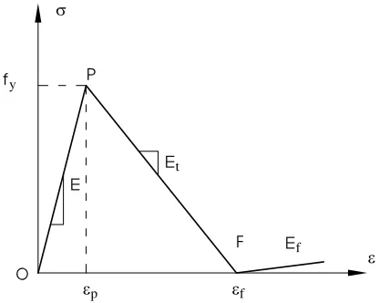
The material behaviour is described by a bilinear constitutive law as presented in Fig. 2, which ex-hibits elastic behavior with Young’s modulus E

up to strainεpat the peak stress fy(strength),

fol-lowed by strain-softening (linePF), which has a negative slopeEt up toεf, where the stress has a

value of zero, finally, followed by a nearly hori-zontal tail of a very small positive slopeEf.

The constitutive relation is thus given by

σ(x,t) =Eε, (2)

in whichε =ε(x,t) =∂u_∂(x_x,t)is the strain andEis the slope of the stress-strain relation, defined by

E=

⎧ ⎪ ⎨ ⎪ ⎩

E, ifε ≤εp,

Et, ifεp≤ε≤εf,

Ef, ifε ≥εf.

(3)

The boundary conditions are

u(x=−L,t) =−ct; u(x=L,t) =ct, fort≥0. (4)

Figure 2: A constitutive relation for quasi-brittle materials.

The initial solutions are taken as follows

u(x,t=0) =0 and ∂u(x,t=0)

∂t =0,

for −L≤x≤L. (5)

Due to symmetry, the problem is equivalent to a bar fixed atx=0. Thus the boundary conditions for a half model now become

u(x=−L,t) =−ct; u(x=0,t) =0, fort≥0. (6)

The governing equations are non-dimensionalised using the following scheme: characteristic length

a; characteristic timeT=_va

e, whereve=

E/ρis the elastic wave speed; characteristic stressσc=

E; velocities are normalised by ve, e.g. c/ve is

the dimensionless loading velocity at the ends of the bar. The dimensionless momentum equation is given by

∂2_u(x,t)

∂t2 =

ET2

ρa2

∂σ(x,t)

∂x , =

E E

γ2∂ε(x,t)

∂x , (7)

whereEis given in Eq. 3,γ= ET_ρa22 =

veT

a .

3 Numerical formulation

Consider an initial-boundary-value problem gov-erned by the second order PDE

∂u

∂t =q1

∂2_u

∂x2+q2

∂u

∂x+q3u+q4, (8)

whereq1, q2,q3andq4are the coefficients, 0≤

t≤T andxmin≤x≤xmax, with the boundary and

initial conditions

u(t,x=xmin) =u1, (9)

∂u

∂x|(t,x=xmax)=u

N, (10)

u(0,x) =g(x), (11)

in whichu1anduNare given values, andg(x)is a

known function.

3.1 Spatial discretisation

In the indirect RBF method (see [Mai-Duy and Tran-Cong (2001, 2005); Duy (2005); Mai-Duy and Tanner (2005)]), the formulation of the problem starts with the decomposition of the highest order derivative under consideration into RBFs. The derivative expression obtained is then integrated to yield expressions for lower order derivatives and finally for the original function it-self. The present work is concerned with the ap-proximation of a function and its derivatives of or-der up to 2, the formulation can be thus described as follows [Mai-Cao and Tran-Cong (2005); Le, Mai-Duy, Tran-Cong, and Baker (2007)]

d2u(x,t) dx2 =

m

∑

i=1

wi(t)gi(x) = m

∑

i=1

wi(t)Hi[2](x),(12)

du(x,t)

dx =

m

∑

i=1

wi(t)gi(x)dx+c1(t)

=

∑

i=1 wi(t)

gi(x)dx+c1(t)

=

∑

i=1

wi(t)Hi[1](x) +c1(t), (13)

u(x,t) =

m

∑

i=1 wi(t)

H_i[1](x)dx+c1(t)x+c2(t)

=

∑

i=1

wi(t)Hi[0](x) +c1(t)x+c2(t),(14)

wheremis the number of RBFs,{gi(x)}mi=1is the

set of RBFs, {wi(t)}mi=1 is the set of

correspond-ing network weights to be found and{H_i[j](x)}m_i=1

(j=0,1) are new basis functions obtained from integrating the radial basis functiongi(x)once or

more times. The multiquadrics function is chosen in the present study

gi(x) = (x−ci)2+a2i, (15)

where ci is the RBF centre and ai is the RBF

width. The width of the ith RBF can be deter-mined according to the following simple relation

ai=βdi, (16)

whereβ is a factor,β >0, anddi is the distance

from theith centre to its nearest centre. To have the same coefficient vector as Eq. 14, Eq. 12 and Eq. 13 can be rewritten as follows

d2_u(x,t) dx2 =

m

∑

i=1

wi(t)Hi[2](x) +c1(t).0+c2(t).0,

(17)

du(x,t)

dx =

m

∑

i=1

wi(t)H[

1]

i (x) +c1(t).1+c2(t).0.

(18)

Here we choose the RBF centrescito be identical

to the collocation pointsxi, i.e.{ci}m_i=1={xi}N_i=1.

The evaluation of Eq. 17, Eq. 18 and Eq. 14 at a set ofNcollocation points leads to

u(t) = H[2]w(t), (19)

u(t) = H[1]w(t), (20)

u(t) = H[0]w(t), (21)

where

u(t) =

∂2_u1(t)

∂x2 ,

∂2_u2(t)

∂x2 ,...,

∂2_u

N(t)

∂x2

T

, (22)

u(t) =

∂u1(t)

∂x ,

∂u2(t)

∂x ,...,

∂uN(t)

∂x

T

, (23)

H[2]= ⎛ ⎜ ⎜ ⎜ ⎜ ⎝

H₁[2](x1) H₂[2](x1) ··· H_N[2](x1) 0 0

H₁[2](x2) H₂[2](x2) ··· H_N[2](x2) 0 0 ..

. ... . . . ... ... ...

H₁[2](xN) H₂[2](xN) ··· HN[2](xN) 0 0

⎞ ⎟ ⎟ ⎟ ⎟ ⎠, (25)

H[1]=

⎛ ⎜ ⎜ ⎜ ⎜ ⎝

H₁[1](x1) H₂[1](x1) ··· H_N[1](x1) 1 0

H₁[1](x2) H₂[1](x2) ··· H_N[1](x2) 1 0 ..

. ... . . . ... ... ...

H₁[1](xN) H₂[1](xN) ··· H_N[1](xN) 1 0

⎞ ⎟ ⎟ ⎟ ⎟ ⎠, (26)

H[0]=

⎛ ⎜ ⎜ ⎜ ⎜ ⎝

H₁[0](x1) H₂[0](x1) ··· H_N[0](x1) x1 1 H₁[0](x2) H₂[0](x2) ··· H_N[0](x2) x2 1

..

. ... . . . ... ... ...

H₁[0](xN) H[

0]

2 (xN) ··· H[

0]

N (xN) xN 1

⎞ ⎟ ⎟ ⎟ ⎟ ⎠, (27) and

w(t) = [w1(t),...,wN(t),c1(t),c2(t)]T. (28)

From an engineering point of view, it would be more convenient to work in the physical space. Owing to the presence of integration constants, the process of converting the networks-weight space into the physical space can also be used to implement Neumann boundary conditions. With the boundary conditions Eq. 9 and Eq. 10, the conversion system can be written as

u(t) u_N(t)

=Cw(t), (29)

where C is the conversion matrix of dimension

(N+1)×(N+2)that comprises the matrixH[0]

and the last row ofH[1]_{. Solving Eq. 29 yields}

w(t) =C−1

u(t) u_N(t)

. (30)

By substituting Eq. 30 into Eq. 19 and Eq. 20, the values of the second and first derivatives ofuwith respect tox are thus expressed in terms of nodal variable values and Neumann boundary values

u(t) =H[2]C−1

u(t) u_N(t)

=D[2]

u(t) u_N(t)

, (31)

u(t) =H[1]C−1

u(t) u_N(t)

=D[1]

u(t) u_N(t)

. (32)

Making use of Eq. 31 and Eq. 32, Eq. 8 can be transformed into the following discrete form

du(t) dt =q1u

_{(t) +q2u(t) +q3u(t) +q}

4, (33)

or

du dt =q1D

[2]

u(t) u_N(t)

+q2D[1]

u(t) u_N(t)

+q3u(t) +q4, (34)

whereq4= [q4,q4,...q4]Tis anN×1 vector, and

du dt =

du1(t) dt ,

du2(t) dt ,...,

duN(t)

dt

T

. (35)

Since the values ofu1 andu_N are given, the un-known vector becomes

[u2(t),u3(t),...,uN(t)]T, (36)

and hence, the first row in Eq. 34 will be removed from the solution procedure. The remainder of Eq. 34 can be integrated in time by using standard solvers such as the Runge-Kutta technique.

3.2 Regularization of IRBFNs and capturing of discontinuous strains

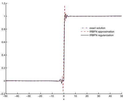
and Liu (2000)]. On the other hand, several mesh-free methods used special shape functions to ac-count for the jump across a discontinuity [Kron-gauz and Belytschko (1998); Kim, Liu, Yoon, Be-lytschko, and Lee (2007)], which seem to work well if the location of discontinuities are known. It will be seen that the present IRBFN method can capture strain discontinuities without suffer-ing any mesh-alignment sensitivities (IRBFN is a truly meshless method) and without having to know the location of discontinuities in advance. However, being a global and high order approxi-mation, the RBFN still produce some oscillations around the discontinuity (Fig. 3). In this study we introduce a new approach where RBFNs can be further regularised to alleviate oscillatory be-haviours near such discontinuities.

−50 −40 −30 −20 −10 0 10 20 30 40 50 −0.2

0 0.2 0.4 0.6 0.8 1 1.2

x

exact solution IRBFN approximation IRBFN regularization

Figure 3: Regularization of IRBFNs.

With noisy data, the generalization performance of RBFNs can be improved using regular-ization techniques presented in [Orr (1995b)],

which are adapted here for IRBFNs. Let

(x={xi}N_i=1,ˆy={yˆi}N_i=1)

denote the set of in-put and f(x) the output in the present IRBFN method, the sum-squared-error is

S=

N

∑

i=1

(yˆi−f(xi))2, (37)

whereNis the number of input data points, f(xi)

is the approximate solution given by Eq. 14 (or

Eq. 21 in matrix form). The output sensitivity to noisy inputs is minimised by augmenting the sum-squared-error with a smoothing term [Orr (1995b)] as follows.

C=

N

∑

i=1

(yˆi−f(xi))2+λ m

∑

j=1

w2_j, (38)

where C is a cost function, m is the number of RBF centres,wj are the network weights,λ is a

non-negative regularization parameter. An opti-mal weight vector w can be found by minimiz-ingCin Eq. 38 with respect to network weights

wj

N

j=1 as follows. Differentiating the cost

functionC with respect to the network weights

wj

N

j=1yields

∂C

∂wj =−

2

N

∑

i=1

(yˆi−f(xi))∂

f(xi)

∂wj +

2λ

m

∑

j=1 wj.

(39)

From Eq. 14 or Eq. 21, ∂f(xi)

∂wj in Eq. 39 can be

found simply as

∂f(xi)

∂wj =

H[_j0](xi), (40)

or in compact form

∂f

∂wj =

h[_j0], (41)

where

f= [f(x1),f(x2),...,f(xN)]T, (42)

and

h[_j0]=

H[_j0](x1),H_j[0](x2),...,H[_j0](xN)

T

. (43)

Note that vectorh[_j0]is the j-th column of the ma-trixH[0]in Eq. 27. Substituting Eq. 41 into Eq. 39 and equating the results to zero lead to

N

∑

i=1

f(xi)H[

0]

j (xi) +λwj=

N

∑

i=1 yiH[

0]

j (xi). (44)

There are m such equations corresponding tom

one constraint on the solution. The resultant sys-tem of linear equations like Eq. 44 can be rewrit-ten in matrix form,

H[0]

T

f+λIm+2w=

H[0]

T

ˆy, (45)

in whichIm+2 is an identity matrix of size (m+

2)×(m+2). Solving Eq. 45 leads to the vector of optimal weights

w=A−1

H[0]

T

ˆy, (46)

where

A=

H[0]

T

H[0]+λIm+2. (47)

Since the performance of the IRBFN regulariza-tion completely depends on the regularizaregulariza-tion pa-rameter λ, an optimal λ must be identified to minimise the error. A number of methods pre-dicting an optimal value ofλ automatically have been developed [Orr (1995a,b, 1996)] including the re-estimation method using different error pre-diction criteria, (e.g. cross-validation, generalized cross-validation, Bayesian information criterion, final prediction error, unbiased estimate of vari-ance). In the present work, the generalized cross-validation (GCV) error prediction criterion is em-ployed as follows.

ˆ

σ2₌ NˆyTP2ˆy

[trace(P)]2, (48)

where ˆσ2_{is the variance estimate,Nis the number}

of input data points, P is the projection matrix, which is defined by

ˆy−f=ˆy−H[0]A−1

H[0]

T

ˆy=P ˆy, (49)

in whichP=IN−H[0]A−1

H[0]T,INis an

iden-tity matrix of size N×N. ThusP relates to the sum-square-errorSby

S=ˆyTP2ˆy, (50)

and the cost functionCby

C=ˆyTP ˆy. (51)

Since all the above error prediction criteria relate nonlinearly toλ, a method of nonlinear optimiza-tion is required for the estimaoptimiza-tion ofλ. Any stan-dard technique of nonlinear optimization such as the Newton method can be used in this circum-stance. Alternately, the optimal value of λ can automatically be determined by a simple iterative procedure [Orr (1996)] as follows.

By differentiating the GCV error prediction and setting the results to zero, a nonlinear equation of λ can be obtained. After some mathematical ma-nipulations,λ can be found iteratively as

λ = ˆyTP2ˆy trace

A−1−λA−2

wT_A−1_{w trace}(_P) , (52)

where the right hand side contains λ (explicitly as well as implicitly through A−1 and P). The iterative procedure is started with an initial value ofλ for the computation of the right hand side, which is a new estimate ofλ, and the process is repeated until convergence.

0 0.1 0.2 0.3 0.4 0.5 0.6 0.7 0.8 0.9 1 −1.5

−1 −0.5 0 0.5 1 1.5

x

y

RBFN regularization

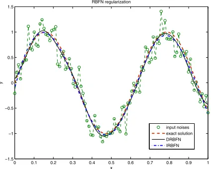
input noises exact solution DRBFN IRBFN

Figure 4: Noisy input, exact solution, DRBFN regularization and IRBFN regularization.

y=sin(10x), for 0≤x≤1, with additional Gaus-sian noise of standard deviation σ =0.20 (the curve with circular marker in Fig. 4). The tar-get (exact) function y=sin(10x) is depicted by the dash curve. As shown in Fig. 4, the IRBFN regularization method provides a better result (the dot-dash curve) with the mean square error (eM)

of 0.0022 compared with 0.0033 of the DRBFN method (the continuous curve), where eM is

de-fined as

eM=∑ N

i=1(f(xi)−yi)2

N , (53)

in whichNis the number of test nodes (N=300),

f(xi) the output value and yi the exact value of

the target function. This results is also in good agreement with those of [Mai-Duy (2005)], which showed that the IRBFN method obtained by in-tegration process leads to a better approximation than the DRBFN method by differential process.

4 Numerical examples

For all computations presented in this section, the common dimensionless parameters are chosen as

L=50, γ2=

ET2

ρa2

=1,εp=1,

fy=1,

Et

E

=−0.70, εf =2.4286,

Ef

E

=10−6.

Those parameters that are specific to each exam-ple are described later where appropriate.

4.1 Wave propagation in fully elastic bars

A uniform bar is loaded by an extensional velocity

cof the two ends as shown in Fig. 1. Longitudinal elastic wave propagation precedes strain localisa-tion and is considered in this example. Moreover, ifcsatisfies the conditionc≤εp/2, the behaviour

of the bar is purely elastic over the whole compu-tational domain [Bazant and Belytschko (1985)]. The differential equation of motion Eq. 7 reduces to (in dimensionless form)

∂2_u(x,t)

∂t2 =γ

2∂2u(x,t)

∂x2 , (54)

which is hyperbolic. The exact solution of Eq. 54 for the given boundary conditions Eq. 4 and the initial solutions Eq. 5 can be found in [Bazant and Belytschko (1985)] and presented for the dis-placementuand strainε as follows.

u=−cγt−(x+L)+cγt+(x−L),

0≤t≤

1 γ

2L, (55)

where the symbolis defined by

A=

A, ifA≥0,

0, ifA<0, (56)

and

ε=∂_∂u x

=c[H(γt−(x+L))] +c[H(γt+(x−L))],

(57)

in whichH denotes the Heaviside step function, defined by

H(x) =

1, ifx≥0,

0, ifx<0. (58)

The governing equation Eq. 54 involves second-order derivatives of both space and time, and it is convenient to decouple it into a system of first-order equations in both space and time by intro-ducing new variablesrandsas follows. Let

r=γ∂u

∂x, s=

∂u

∂t, (59)

and Eq. 54 is thus equivalent to the system of equations

∂r

∂t =γ

∂s

∂x, (60)

∂s

∂t =γ

∂r

∂x, (61)

subject to the corresponding boundary conditions

s(−L,t) =−c, s(L,t) =c, ∀t∈

0,

1 γ

2L

,

and the initial solutions

r(x,0) =0, s(x,0) =0, ∀x∈[−L,L]. (63)

To reduce the computational cost, a half model is analyzed in this section. The equivalent boundary conditions of the half model are

s(−L,t) =−c, s(0,t) =0,

∀t∈

0,

1 γ

2L

, (64)

The numerical formulation presented in section 3 is used for solving the system of equations Eq. 60 and Eq. 61 with the boundary conditions Eq. 64 and the initial solutions Eq. 63, withc=0.45εp.

The forward Euler formula is used to perform time integration. To satisfy the CFL condition (t ≤ 1_γx), the time step is chosen as t =

10−2 1

γxin this example. The results presented in this example are achieved with 80 uniform col-location points and β =1 in Eq. 16. Computa-tions are also carried out with 20, 40, 60 and 100 uniformly distributed collocation points. The ob-tained solution essentially converges when 40 or more collocation points are used. Fig. 5, Fig. 6 and Fig. 7 show the evolution of the displace-ment and strain, the numerical results and the exact solutions are plotted on the same graphs. First, the displacement and strain waves propa-gate from the ends to the center of the bar until these incident waves meet each other at the cen-ter at timet=

1

γ

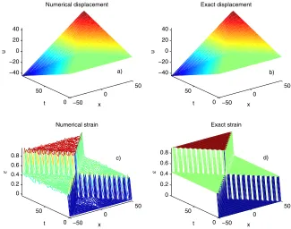
L. The zero-th order continu-ous displacement leads to the strain discontinuity whose position evolves with time as shown in the above figures. As a result of the collision of the two incident waves (atx=0), an abrupt jump of value of strain appears atx=0 (Fig. 8), the strain magnitude is doubled, and the reflection waves propagate outwards to the ends as displayed in Fig. 5(e)-(f)-(g)-(h), Fig. 7 and Fig. 8. The ob-tained results by the present IRBFN method are in good agreement with the analytical solutions as shown in Fig. 5-Fig. 8.

It is shown that the IRBFN can capture the dis-continuous strain in this example, however, there are some oscillations due to the violation of the

smoothness assumption inherent in the RBFN ap-proximation. This situation can be improved with regularisation as discussed in section 3.2. When the regularisation parameter λ is set to be equal to 0.07135, it can be seen that the obtained strains shown on the right columns in Fig. 6 and Fig. 7 are much smoother and closer to the exact solu-tions than those by the standard IRBFN method shown on the left columns of the same figures. Thus, good results are achieved with a general global regularisation of the IRBFNs in contrast with other numerical approaches (discussed in section 3.2) where special treatments must be ap-plied at the elemental level (extended FEM) or special shape functions must be used. Moreover, these special treatments require a priori knowl-edge of the location of discontinuities while the present IRBFN method does not.

4.2 Wave propagation and strain localization in strain-softening bars: local continuum model

In this example, the problem defined in section 2 is considered with the prescribed velocities at the ends havec=0.85εp, which is above the critical

value of 0.5εp. The behaviour of the bar is

elas-tic until the incident waves meet at the center of the bar (i.e. for 0≤t≤L) as discussed in sec-tion 4.1. Right after the collision of the incident waves, the strain is doubled to 2c=1.7εp, causing

strain softening and strain localization. From the onset of localization, the computational domain can be divided into two regions with different be-haviors: the strain softening and localization zone and the elastic zone. For the elastic domain, the momentum equation Eq. 7 takes the hyperbolic form of Eq. 54 which is solved in the same manner as presented in section 4.1. For the localized zone, the momentum equation becomes elliptic and is solved by a scheme described as follows.

The elliptic momentum equation of the localized zone is

∂2_u(x,t)

∂t2 =−μ

2∂2u(x,t)

∂x2 , (65)

in which μ2 = |Et|

E ET2

−50 0 50 −5

0 5

x

u

t = 17.2685

−50 0 50

−10 0 10

x

u

t = 26.1350

−50 0 50

−10 0 10

x

u

t = 35.0015

−50 0 50

−10 0 10

x

u

t = 43.8680

−50 0 50

−20 0 20

x

u

t = 61.6011

−50 0 50

−20 0 20

x

u

t = 70.4676

−50 0 50

−20 0 20

x

u

t = 79.3341

−50 0 50

−40 −20 0 20 40

x

u

t = 92.6339

a) b)

c) _d)

e) f)

g)

h)

Figure 5: Fully elastic bars: the evolution of displacement, the continuous curves denote the IRBFN solu-tions and the dash ones the exact solution.

−50 0 50

0 0.2 0.4

x

ε

t = 17.2685

−50 0 50

0 0.2 0.4

x

ε

t = 17.2685

−50 0 50

0 0.2 0.4

x

ε

t = 26.1350

−50 0 50

0 0.2 0.4

x

ε

t = 26.1350

−50 0 50

0 0.2 0.4

x

ε

t = 35.0015

−50 0 50

0 0.2 0.4

x

ε

t = 35.0015

−50 0 50

0 0.2 0.4

x

ε

t = 43.8680

−50 0 50

0 0.2 0.4

x

ε

t = 43.8680

a1) a2)

b1) b2)

d1)

c2) c1)

d2)

−50 0 50 0.5

0.6 0.7 0.8 0.9

x

ε

t = 61.6011

−50 0 50

0.5 0.6 0.7 0.8 0.9

x

ε

t = 61.6011

−50 0 50

0.4 0.6 0.8

x

ε

t = 70.4676

−50 0 50

0.4 0.6 0.8

x

ε

t = 70.4676

−50 0 50

0.5 0.6 0.7 0.8 0.9

x

ε

t = 79.3341

−50 0 50

0.5 0.6 0.7 0.8 0.9

x

ε

t = 79.3341

−50 0 50

0.5 0.6 0.7 0.8 0.9

x

ε

t = 92.6339

−50 0 50

0.5 0.6 0.7 0.8 0.9

x

ε

t = 92.6339

e1) e2)

f1) f2)

g1) _g2)

h1) h2)

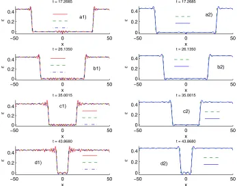
Figure 7: Fully elastic bars: the propagation of step function waves of strain: the continuous curves de-note the IRBFN solutions, the dashed ones exact solutions and the dot-dashed curves indicate the IRBFN regularized results on the left column. On the right column, the non-regularized results are removed for clarity.

−50 0

50

0 50 −40 −20 0 20 40

x Numerical displacement

t

u

−50 0

50

0 50 −40 −20 0 20 40

x Exact displacement

t

u

−50 0

50

0 50 0 0.2 0.4 0.6 0.8

x Numerical strain

t

ε

−50 0

50

0 50 0 0.2 0.4 0.6 0.8

x Exact strain

t

ε

a) b)

c) d)

of first-order equations in both time and space by letting

r=−μ∂u

∂x, s=

∂u

∂t, (66)

resulting in a system of equations inr ands for the strain-softening zone given by

∂r

∂t =−μ

∂s

∂x, (67)

∂s

∂t =μ

∂r

∂x. (68)

At the end of the softening process, fracture and rupture will probably occur, however, a fracture criterion is not included in present study, so the material is assumed to be elastic again with a very small elastic modulusEf/E=10−6. The

govern-ing equations in this stage are the same as those in section 4.1, except that the modulusE is re-placed byEf. As before, only a half model needs

be discretised (in this case with 80 uniformly dis-tributed nodes). The resultant system of equations is integrated in time by using the forward Euler formula as in section 4.1, where the time step is taken as t =0.25×10−4_γx in this example. The solution of Eq. 67 and Eq. 68 clearly shows the onset of strain localization, characterized by the sudden jump in velocity, displacement, strain and the rapid descent of stress in the localized zone as exhibited in Fig. 9 which depicts the evo-lution of velocity, displacement, strain and stress at the collocation pointx=−0.6329, which is the nearest point to thex=0 node. In Fig. 9(d), the stress profile is slightly oscillatory until the load-ing waves are about to meet. Upon the collision of the incident waves, the stress increases rapidly to the elastic limit fy then decreases as rapidly

down to zero again due to strain-softening. The speedy drop of the stress level is accompanied by the abrupt jump in velocity and rapid increase in displacement and strain as exhibited in Fig. 9(c)-(a)-(b), respectively. Unstable development fol-lows as the localized zone is unable to carry load while the velocity is increasing, the displacement and strain are growing rapidly, two halves of the bar are moving increasingly in two opposite direc-tions like in mode I crack as shown in Fig. 10. In

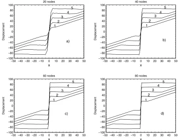
the next stage of evolution, the velocity and stress increase very slightly while the displacement and strain are growing continuously and quickly be-cause of elastic loading as can be seen in Fig. 9. The steep profiles of stress, velocity and strain are well captured by the present explicit method, although with smaller time steps in comparison with other implicit methods. Fig. 10-Fig.12 depict the spatio-temporal evolution of the displacement, velocity and strain, respectively, while Fig. 13-Fig. 15 show the spatial distribution of velocity, stress, displacement and strain, respectively, at several time instants. The solutions of the ellip-tic equations yield a standing wave, which is not able to extend outside the localised zone, as illus-trated by the strain wave displayed in Fig. 12 and Fig. 15, and the displacement wave in Fig. 10 and Fig. 14 as well. When softening occurs, which is the case here, the localised strain softening zone causes reflection waves travelling backwards from the localised front (x=0), due to sudden unload-ing.

Fig. 10 and Fig. 14 expose the development of displacement which grows rapidly as a stand-ing wave confined in a very narrow zone. Cor-respondingly, the increasingly intensive strain within the localized zone is depicted in Fig. 12 and Fig. 15. The velocity is doubled at the on-set of localisation and reflected back from the lo-calised zone as shown in Fig. 11 and Fig. 13(a). Similarly, displacement, strain and stress waves also reflected from the localised zone. However, unlike the response in purely elastic bars, the reflected strain wave is out of phase with, and therefore cancelling out the incident strain wave of the same magnitude. Due to the nature of the displacement waves the displacement field in the elastic region isC0 continuous (Fig. 10 and Fig. 14). The point ofC0continuous displacement propagates along the elastic region in both direc-tions depending on the stage of loading. Conse-quently, a discontinuity occurs in the profile of stress, velocity (Fig. 13), and strain (Fig. 15). The oscillatory behaviour of the stress is observed in Fig. 13(b) which was also found in [Sluys (1992); Bazant, Belytschko, and Chang (1984)].

0 10 20 30 40 50 60 70 80 90 100 −80

−60 −40 −20 0

x = −0.6329, 80 nodes

t

Displacement

0 10 20 30 40 50 60 70 80 90 100

0 20 40 60

x = −0.6329, 80 nodes

t

Strain

0 10 20 30 40 50 60 70 80 90 100

−1.4 −1.2 −1 −0.8 −0.6 −0.4 −0.2 0 0.1

x = −0.6329, 80 nodes

t

Velocity

0 10 20 30 40 50 60 70 80 90 100

−0.1 0 0.2 0.4 0.6 0.8 1 1.2

x = −0.6329, 80 nodes

t

Stress

a) b)

c) d)

Figure 9: Local continuum model: the evolution of: (a) displacement, (b) strain, (c) velocity and (d) stress atx=−0.6329 with 80 uniform collocation points.

−50 0

50

0 10 20 30 40 50 60 70 80 90 100 −100

−50 0 50 100

x 80 nodes

t

Displacement

−50 0

50

0 20

40 60

80 100

−2 −1.5 −1 −0.5 0 0.5 1 1.5 2

t 80 nodes

x

Velocity

Figure 11: Local continuum model: the evolution of velocity with a uniform discretisation of 80 points.

−50

0

50

0 20 40 60 80 100 −10 10 30 50 70 90 110 130 150 170

x 80 nodes

t

Strain

−50 −40 −30 −20 −10 0 10 20 30 40 50 −2

−1.5 −1 −0.5 0 0.5 1 1.5 2

80 nodes

x

Velocity

−50 −40 −30 −20 −10 0 10 20 30 40 50

−0 0.2 0.4 0.6 0.8 1 1.2

80 nodes

x

Stress

a)

b)

1

1 2 3 4

5

2 3 4

5

Figure 13: Local continuum model: the curve labels represent time levels: 1(t =60.0) ; 2(t=70.0) ; 3(t=80.0) ; 4(t=90.0) ; 5(t=100.0) (a) the evolution of velocity, (b) stress obtained with a uniform discretisation of 80 points.

−50 −40 −30 −20 −10 0 10 20 30 40 50

−100 −80 −60 −40 −20 0 20 40 60 80 100

20 nodes

x

Displacement

−50 −40 −30 −20 −10 0 10 20 30 40 50

−100 −80 −60 −40 −20 0 20 40 60 80 100

40 nodes

x

Displacement

−50 −40 −30 −20 −10 0 10 20 30 40 50

−100 −80 −60 −40 −20 0 20 40 60 80 100

60 nodes

x

Displacement

−50 −40 −30 −20 −10 0 10 20 30 40 50

−100 −80 −60 −40 −20 0 20 40 60 80 100

80 nodes

x

Displacement

a) b)

c) d)

5 1

2 3

4 5

1 2

3 4

5

1 2

3 4

5

1 2

3 4

−50 −40 −30 −20 −10 0 10 20 30 40 50 −5

0 5 10 15 20 25 30 35 40

20 nodes

x

Strain

−50 −40 −30 −20 −10 0 10 20 30 40 50

0 10 20 30 40 50 60 70 80

40 nodes

x

Strain

−50 −40 −30 −20 −10 0 10 20 30 40 50

0 20 40 60 80 100 120

60 nodes

x

Strain

−50 −40 −30 −20 −10 0 10 20 30 40 50

0 20 40 60 80 100 120 140 160 180

80 nodes

x

Strain

−50 −40 −30 −20 −10 0 10 20 30 40 50

0 20 40 60 80 100 120

60 nodes

x

Strain

a) b)

c) d)

1 2 3 4 5

1 3

2 4 5

1 3

2 4 5

1 2 3 4 5

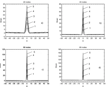
Figure 15: Local continuum model: the evolution of strain at time levels: 1(t=60.0) ; 2(t=70.0) ; 3(t=

80.0) ; 4(t=90.0) ; 5(t=100.0) (a) 20 points, (b) 40 points, (c) 60 points and (d) 80 points (uniformly discretised).

to an 80 point discretisation, computation is also carried out for 20, 40, 60, 100, 120 point dis-cretisations. As the number of collocation points increases, the bandwidth of the localised zone decreases and the maximum strain increases as shown in Fig. 14 and Fig. 15, which is a trend predicted by the exact solution [Bazant and Be-lytschko (1985)]. However, the zero bandwidth and singular strain associated with the exact model solution cannot be expected to be captured by a numerical method. The obtained results in this section compare favourably with those of the FEM [Sluys (1992); Bazant, Belytschko, and Chang (1984)]. It is worth noting that, unlike the FEM, the present method does not require a pri-ori knowledge of the location of discontinuities which are well captured by a uniform discretisa-tion.

4.3 Wave propagation and strain localization in strain-softening bars: non-local contin-uum model

In this example, the material is described by a non-local continuum model based on strain aver-aging or non-local strain. In this model, the lo-cal equivalent strainε is replaced by its non-local counterpart obtained by a weighted average pro-cess over a spatial neighbourhood of each point of interest. The non-local strainε is defined by

ε(x,t) =

Vα(

x,ξ)ε(ξ,t)dξ, (69)

con-dition

Vα(

x,ξ)dξ=1, ∀x∈V. (70)

This can be achieved by setting

α(x,ξ) = α0(x−ξ )

Vα0(x−ζ )dζ

, (71)

whereα0(r)is an even and non-negative function of the distancer =x−ξ , monotonically de-creasing forr≥0. It is often taken as the piece-wise polynomial bell-shaped function

α0(r) =

⎧ ⎨ ⎩

1−_Rr22

2

, if 0≤r≤R, 0, ifr>R,

(72)

where R is a parameter related to the internal length of the material. SinceRcorresponds to the maximum distance of pointξthat affects the non-local average at pointx, it is called theinteraction radius[Patzák and Jirásek (2003)].

The stress-strain relation in Eq. 2 becomes (in di-mensionless form)

σ(x,t) = E

Eε(x,t), (73)

whereε is the non-local strain. Thus the stress in Eq. 73 is also non-local. In order to evaluateε, it is necessary to computeε(ξ,t)in Eq. 69, which is accomplished as follows. After an IRBFN cretisation, the vectors of unknown nodal dis-placements and their corresponding first and sec-ond derivatives with respect to x are given by Eq. 21, Eq. 32 and Eq. 31, respectively. Thus, the first order derivative of the displacement with respect toxat an arbitrary pointξ can be written as follows.

∂u(ξ,t)

∂x =ε(ξ,t) =H

[1]_(ξ)C−1_u(t)

=D[1](ξ)u(t), (74)

where C−1 _{and u(t) are given by Eq. 30 and}

Eq. 21, respectively. H[1](ξ)andD[1](ξ)are ob-tained in the same manner that leads toH[1] and

D[1]in Eq. 32, but with x =ξ. Substitution of Eq. 74 into Eq. 69 leads to

ε(x,t) =

R

−Rα(

x,ξ)D[1](ξ)u(t)dξ. (75)

Since the nodal variable vector u(t) is indepen-dent of the spatial variable, Eq. 75 can be rewrit-ten as

ε(x,t) =

_R

−Rα(

x,ξ)D[1](ξ)dξu(t) =B(x)u(t),

(76)

where

B(x) =

R

−Rα(

x,ξ)D[1](ξ)dξ. (77)

The momentum equation Eq. 7 becomes

∂2_u(x,t)

∂t2 =

E E

ET2

ρa2

∂σ(x,t)

∂x , (78)

which, in the elastic case, reduces to

∂2_u(x,t)

∂t2 =γ

2∂ε(x,t)

∂x . (79)

Since the stress and strain are non-local, a new system of governing equations is derived by de-coupling the momentum equation Eq. 79 as fol-lows. Let

r=γε(x) =γB(x)u(t), s=∂u

∂t. (80)

After discretisation, the unknown nodal vectors forrandsare, respectively,

r(t) = [r1(t),r2(t),...,rN(t)]T, (81)

and

s(t) = [s1(t),s2(t),...,sN(t)]T, (82)

whereNis the number of collocation points. From Eq. 80 and Eq. 82, we have

∂u(t)

∂t =s(t). (83)

From Eq. 79, Eq. 80 and Eq. 83, the following system of governing equations, which is equiva-lent to Eq. 79 (i.e. the elastic case), is obtained

∂r(t)

∂s(t)

∂t =γ

∂r

∂x, (85)

where

B= [B(x1),B(x2),...,B(xN)]T, (86)

with B(xi) =

_R

−Rα(xi,ξ)D[1](ξ)dξ, fori=

1,N

and∂_∂r_x is obtained by an IRBFN approximation as

∂r(t)

∂x =D

[1]_{r(t). (87)}

For the softening response, the corresponding sys-tem of governing equations is

∂r(t)

∂t =−μBs(t), (88)

∂s(t)

∂t =μ

∂r

∂x. (89)

The boundary and initial conditions for r and s

are the same as those given in section 4.2. As can be seen in the previous two examples, the ramp-like spatial displacement profile results in a discontinuous strain field which can be well cap-tured by the present IRBFN method. However, when a non-local continuum model is used here, the smoothness of the equivalent non-local strain is adversely affected by noises that might exist in the neighbouring strain field. Thus it is found to be advantageous to incorporate IRBFN regulari-sation into the general IRBFN formulation. The effect of such regularisation is illustrated by con-sidering a ramp function given by

ˆ

u(x) =xH(x), for −50≤x≤50, (90)

where H is the Heaviside function defined in Eq. 58. The exact solution of the first order deriva-tive of ˆu(x)with respect toxis

ˆ

ε(x) = ∂uˆ(x)

∂x =H(x). (91)

Let ˜ε(x) denote the IRBFN approximation of ∂uˆ(x)

∂x , which is determined by

˜

ε(x)≈∂uˆ(x)

∂x =D

[1]_{(x)uˆ(x), (92)}

The weighted average of ˜ε(x), denoted by ˜ε(x), is achieved by replacingε(ξ,t)in Eq. 69 by ˜ε(x)

˜ ε(x) =

Vα(

x,ξ)ε˜(x)dξ, (93)

The domain is discretised with a uniform distri-bution of 161 collocation points. The IRBFN parameter β =1 in Eq. 16, the interaction ra-diusR=5 in Eq. 93 which is integrated with 11-point Gaussian quadrature, and the IRBFN reg-ularisation parameter is λ =3.391895. The re-sults shown in Fig. 16 demonstrate the effective-ness of the present method. In this figure, the exact solution ˆε(x) is represented by the Heav-iside curve; the dot-dashed curve indicates the IRBFN solution ˜ε(x); the solid curve represents the weighted average of the IRBFN approxima-tion ˜ε(x); the heavy dashed curve represents the regularised weighted average ˜ε(x). The above specific parameters, exceptλ which is dependent on the number of collocation points, are also used in obtaining the results described below.

Returning to the bar problem, the prescribed end velocities are the same as those given in section 4.2, i.e. c=0.85εp. The time step is 10−3_γx.

−50 −40 −30 −20 −10 0 10 20 30 40 50 −0.2

0 0.2 0.4 0.6 0.8 1 1.2

x

exact solution IRBFN approximation weighted average IRBFN regularization

Figure 16: Example of IRBFN regularization.

−50 0

50

0

20

40

60

80

100 −2

−1.5 −1 −0.5 0 0.5 1 1.5 2

t 161 nodes

x

Velocity

−50

0

50

0 20

40 60

80 100

−100 −80 −60 −40 −20 0 20 40 60 80 100

x 161 nodes

t

Displacement

Figure 18: Non-local continuum model: the evolution of displacement with a uniform distribution of 161 collocation points.

−50

0

50

0 20 40 60 80 100 −1

0 5 10 15

x 161 nodes

t

Non−local strain

−50 −40 −30 −20 −10 0 10 20 30 40 50 −0.2

0 0.2 0.4 0.6 0.8 1

x

Non−local stress

161 nodes

−50 −40 −30 −20 −10 0 10 20 30 40 50

−2 −1.5 −1 −0.5 0 0.5 1 1.5 2

x

Velocity

161 nodes

a)

b)

5

1 2 3 4

5

4 3

2 1

Figure 20: Non-local continuum model: the curve labels represent time levels: 1(t=60.0) ; 2(t=70.0) ; 3(t=80.0) ; 4(t=90.0) ; 5(t=100.0) (a) the evolution of velocity obtained ,( b) stress obtained with a uniform distribution of 161 collocation points

vskip1em

−50 −40 −30 −20 −10 0 10 20 30 40 50

−100 −80 −60 −40 −20 0 20 40 60 80 100

41 nodes

x

Displacement

−50 −40 −30 −20 −10 0 10 20 30 40 50

−100 −80 −60 −40 −20 0 20 40 60 80 100

81 nodes

x

Displacement

−50 −40 −30 −20 −10 0 10 20 30 40 50

−100 −80 −60 −40 −20 0 20 40 60 80 100

121 nodes

x

Displacement

−50 −40 −30 −20 −10 0 10 20 30 40 50

−100 −80 −60 −40 −20 0 20 40 60 80 100

161 nodes

x

Displacement

a) b)

c) d)

1 1

2 3

4 5

2 3

4 5

1 2

3 4

5

1 2

3 4

5

Figure 21: Non-local continuum model: the evolution of displacement at time levels: 1(t=60.0) ; 2(t=

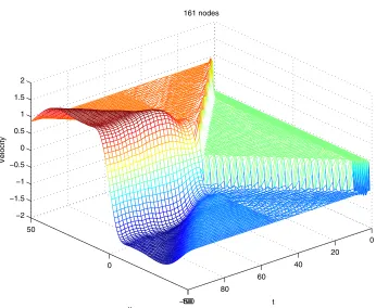
localised zone as shown in Fig. 20-Fig. 22. How-ever, unlike the case of local continuum model, the wave profiles are smooth. In Fig. 20(b), the profiles of stress indicate a complicated loading and unloading process after the initiation of strain localization. There are two narrow zones of high stress at the interfaces between the localized zone and the elastic regions. The standing wave causes the stress to rise in the narrow zones until the elas-tic limit is reached when sudden unloading occurs due to strain softening effect.

Finally, convergence of the present numerical pro-cedure is demonstrated in Fig. 23 where the non-local strain profiles (att=70.0) are displayed for a series of collocation points. As discretisation is refined, it can be seen that the bandwidth con-verges when the number of collocation points is about 160 while the peak non-local strain varies by only 2.3% when the number of collocation points increases from 161 to 241. The slight vari-ation of the peak non-local strain can be expected since the local strain at the centre of the band is singular.

5 Conclusion

An IRBFN meshless method is developed and used to simulate the dynamic strain localization of a bar of quasi-brittle material under dynamic tensile loading. Both local and non-local con-tinuum models are used to describe the material behaviour. The method incorporates a new geral and effective regularization method. The en-hanced IRBFN approach is able to alleviate the effect of noisy data and capture very well weak discontinuities typical of wave propagation and strain localisation. The present method is able to achieve these results using only uniformly dis-tributed collocation points and requiring no prior knowledge of the location of discontinuities.

Acknowledgement: This work is supported by the Australian Research Council. We would like to thank the referees for their helpful comments.

References

Armero, F.; Park, J. (2003): An analysis of strain localization in a shear layer under thermally coupled dynamic conditions. Part 1: Continuum thermoplastic models. international journal for numerical methods in engineering, vol. 56, pp. 2069–2100.

Askes, H.; Bodé, L.; Sluys, L. J.(1998): ALE nanalyses of localization in wave propagation problems. Mechanics of Coheshive-Frictional Materials, vol. 3, pp. 105–125.

Atluri, S.; Shen, S. (2002): The meshless lo-cal Petrov-Galerkin (MLPG) method:A simple & less-costly alternative to the finite element and the boundary element methods. CMES: Computer Modeling in Engineering & Sciences, vol. 3, pp. 11–51.

Atluri, S. N.; Zhu, T.(1998): A new meshless local Petrov-Galerkin (MLPG) approach in com-putational mechanics. Comput. Mech., vol. 22, pp. 117–127.

Batra, R. C.; Zhang, G. M. (2004): Anal-ysis of adiabatic shear bands in elasto-thermo-viscoplastic materials by Modified Smooth-Particle Hydrodynamics (SPH) method. Journal of Computational Physics, vol. 201, pp. 172–190.

Bazant, Z. P.; Belytschko, T. (1985): Wave propagation in a strain softening bar: exact solu-tion. journal of Engineering Mechanics (ASCE), vol. 111, pp. 381–398.

Bazant, Z. P.; Belytschko, T.; Chang, T. P.

(1984): Continuum theory for strain-softening.

journal of Engineering Mechanics (ASCE), vol. 110, pp. 1666–1691.

Driscoll, T. A.; Heryudono, A. R. H. (2007): Adaptive residual subsampling methods for ra-dial basis functions interpolation and collocation problems. Computers & Mathematics with Ap-plications, vol. 53, pp. 927–939.

−50 −40 −30 −20 −10 0 10 20 30 40 50 0

2 4 6 8 10

41 nodes

x

Non−local strain

−50 −40 −30 −20 −10 0 10 20 30 40 50

−1 0 2 4 6 8 10 12 14

81 nodes

x

Non−local strain

−50 −40 −30 −20 −10 0 10 20 30 40 50

−1 0 2 4 6 8 10 12 14

121 nodes

x

Non−local strain

−50 −40 −30 −20 −10 0 10 20 30 40 50

−1 0 2 4 6 8 10 12 14 16

161 nodes

x

Non−local strain

a) b)

c) _d)

2

1 3 4

5

1

1 ₁

2

2 ₂

3

3 ₃

4

4

4 5

5 5

Figure 22: Non-local continuum model: the evolution of non-local strain at time levels: 1(t =60.0) ; 2(t=70.0) ; 3(t=80.0) ; 4(t=90.0) ; 5(t=100.0) (the curve labels indicate time levels) (a) 41 points, (b) 81 points, (c) 121 points and (d) 161 points uniformly discretised.

vskip1em

−50 0 50

0 1 2 3 4 5 6 7

t = 70.0

x

Non−local strain

−50 0 50

0 1 2 3 4 5 6 7

t = 70.0

x

Non−local strain

a) b)

1 2 3 4

4 5

6

Han, Z. D.; Atluri, S. N.(2003): Truly Mesh-less Local Petrov-Galerkin (MLPG) Solutions of Traction & Displacement BIEs. CMES: Com-puter Modeling in Engineering & Sciences, vol. 4, no. 6, pp. 665–678.

Jung, J. H. (2007): A note on the Gibbs phe-nomenon with multiquadratic radial basis func-tions. Applied Numerical Mathematics, vol. 57, pp. 213–229.

Kansa, E. J.(1990): Multiquadrics – a scattered data approximation scheme with applications to computational fluid dynamics – II. Solutions to parabolic, hyperbolic and elliptic partial differen-tial equations. Computers & Mathematics with Applications, vol. 19, pp. 147–161.

Kansa, E. J.; Power, H.; Fasshauer, G. E.; Ling, L. (2004): A volumetric integral radial basis function method for time-dependent partial differential equations: I formulation. Engineer-ing Analysis with Boundary Elements, vol. 28, pp. 1191–1206.

Kim, D. W.; Liu, W. K.; Yoon, Y.; Belytschko, T.; Lee, S. (2007): Meshfree point colloca-tion method with intrisic enrichment for interface problems (in press). Computational Mechanics.

Krongauz, Y.; Belytschko, T.(1998): EFG ap-proximation with discontinuous derivatives. In-ternational Journal for Numerical Methods in En-gineering, vol. 41, pp. 1215–1233.

Le, P.; Mai-Duy, N.; Tran-Cong, T.; Baker, G.

(2007): A numerical study of strain localiza-tion in elasto-therno-viscoplastic materials using radial basis function networks. CMC: Comput-ers, Materials & Continua, vol. 5, pp. 129–150.

Li, S.; Liu, W. C. (2000): Numerical simula-tion of Strain localizasimula-tion in inelastic solids us-ing mesh-free method. International Journal for Numerical Methods in Engineering, vol. 48, pp. 1285–1309.

Ling, L.; Trummer, M. R. (2004): Multi-quadratic collocation method with integral formu-lation for boundary layer problems. Computers &

Mathematics with Applications, vol. 48, pp. 927– 941.

Madych, W. R.; Nelson, S. A. (1990): Mul-tivariate interpolation and conditionally positive definite functions, II. Mathematics of Compu-tation, vol. 54, pp. 211–230.

Mai-Cao, L.; Tran-Cong, T.(2005): A mesh-less IRBFN-based method for transient problems.

CMES: Computer Modeling in Engineering & Sciences, vol. 7, pp. 149–171.

Mai-Duy, N.(2005): Solving high order ordi-nary differential equations with radial basis func-tion networks. International Journal for Numeri-cal Methods in Engineering, vol. 62, pp. 824–852.

Mai-Duy, N.; Khennane, A.; Tran-Cong, T.

(2007): Computation of laminated compos-ite plates using indirect radial basis function net-works. CMC: Computers, Materials & Continua, vol. 5, pp. 63–77.

Mai-Duy, N.; Mai-Cao, L.; Tran-Cong, T.

(2007): Computation of transient viscous flows using indirect radial basis function net-works. CMES: Computer Modeling in Engineer-ing & Sciences, vol. 18, pp. 59–77.

Mai-Duy, N.; Tanner, R. I. (2005): Solving high order partial differential equations with indi-rect radial basis function networks. International Journal for Numerical Methods in Engineering, vol. 63, pp. 1636–1654.

Mai-Duy, N.; Tran-Cong, T.(2001): Numer-ical solution of differential equations using mul-tiquadric radial basic function networks. Neural Networks, vol. 14, pp. 185–199.

Mai-Duy, N.; Tran-Cong, T.(2005): An effi-cient indirect RBFN-based method for numerical solution of PDEs. Numerical Methods for Partial Differetial Equations, vol. 21, pp. 770–790.

Orr, M.(1995a): Local smoothing of radial basis function networks. In International Symposium on Artificial Neural Networks, Hsinchu, Taiwain.

Orr, M.(1995b): Regularisation in the selection of Radial Basis Function Centres. Neural com-putation, vol. 7, pp. 606–623.

Orr, M. (1996): Introduction to radial basis function networks. Tecnical report, Centre for Cognitive Science, University of Edinburgh, Ed-inburgh EH8 9LW, Scotland, 1996.

Patzák, B.; Jirásek, M. (2003): Process zone resolution by extended finite elements. Engineer-ing Fracture Mechanics, vol. 70, pp. 957–977.

Sluys, L. J.(1992): Wave propagation, localisa-tion and dipersion in softening solids. PhD thesis, Delft University of Technology, 1992.

Wen, P.; Hon, Y.(2007): Geometrically nonlin-ear alnalysis of Reissner-Mindlin plate by mesh-less computation. CMES: Computer Modeling in Engineering & Sciences, vol. 21, pp. 177–191.