A second-order continuity domain-decomposition technique based on integrated Chebyshev polynomials for two-dimensional elliptic problems

A second-order continuity domain-decomposition

technique based on integrated Chebyshev

polynomials for two-dimensional elliptic problems

N. Mai-Duy

and T. Tran-Cong

Computational Engineering and Science Research Centre (CESRC)

Faculty of Engineering and Surveying

The University of Southern Queensland, Toowoomba, QLD 4350, Australia

Submitted to

Applied Mathematical Modelling

, February 2007

Abbreviated title:

“A second-order continuity domain-decomposition technique”

∗_{Corresponding author: Telephone +61 7 4631 1324, Fax +61 7 4631 2526, E-mail}

AbstractThis paper presents a second-order (instead of the usual first-order) conti-nuity non-overlapping domain decomposition (DD) technique for numerically solving second-order elliptic problems in two-dimensional space. The proposed DD tech-nique uses integrated Chebyshev polynomials to represent the solution in subdo-mains. The constants of integration are utilized to impose continuity of the second-order normal derivative of the solution at the interior points of subdomain interfaces. To also achieve a C2 _{function at the intersection of interfaces, two additional}

un-knowns are introduced at each intersection point. Numerical results show that the present domain decomposition method yields a higher level of accuracy than con-ventional DD techniques based on differentiated Chebyshev polynomials.

Keywords: Non-overlapping domain decomposition; Second-order continuity; Collo-cation point; Integrated Chebyshev polynomials; Second-order elliptic problems

1

Introduction

Domain decomposition techniques (cf. [1], [2]) are designed to deal with large-scale problems. The problem domain is decomposed into several subdomains, and each subdomain can be analyzed separately. A discretization method used for solving each subdomain is similar to that for a single domain. The use of subdomains facilitates an improvement in the condition number of the system matrix resulting from the discretization of the governing equation. For spectral methods, domain decompositions can also be used for the purpose of handling complex geometries. With the recent emergence of parallel computers, the DD techniques have become more attractive because they allow the parallel implementation of discretization schemes.

com-puted solutions on contiguous regions. The choice between non-overlapping and overlapping subdomains has a profound effect on the computing strategy adopted.

In an overlapping domain technique, only continuity of the function is enforced. The interface solution is solved via an iterative procedure, in which nodal function values at interfaces are updated using previous approximate interior solutions of their neighbouring subdomain. The rate of convergence is an increasing function of the overlap.

In a non-overlapping domain method, continuity of the function and its normal derivative is imposed at selected points along the interfaces. The computed solution is thus considered to be C1 _{continuous across the interfaces. For the case of many}

subdomains, there are further complications due to the presence of interior inter-section points. There are two normal derivatives at an interior corner point, but one has only one equation to enforce their continuity. As a result, special treatment is required. Conventionally, one of these two normal derivatives is left out of the solution process [3].

Spectral methods (cf. [3], [4], [5]) have become increasingly popular in the compu-tation of continuum mechanics problems. For smooth problems, they feature the property of spectral accuracy. In the context of pseudospectral techniques, given a tensor product grid, integrated Chebyshev polynomials were found to be more accurate than differentiated Chebyshev polynomials especially for the solution of high-order problems ([6], [7]).

con-tinuity conditions at the interior corner points (two equations, three unknowns). Karageorghis [9] proposed a fully conforming spectral collocation scheme, where the approximate solution is C1 _{continuous not only at the interior points but also at}

both ends of the interfaces. Unlike DD techniques based on differential formulations (e.g. [3], [9], [10], [11]), the present integral DD technique achieves continuity in the second-order normal derivative of the solution everywhere on the interfaces.

An outline of the paper is as follows. A brief review of the integral collocation formulation using Chebyshev polynomials is given in Section 2. Section 3 describes the proposed DD technique based on integrated Chebyshev polynomials for second-order elliptic problems. Numerical results are presented in Section 4 to verify the formulation and to demonstrate the attractiveness of the proposed DD technique. Section 5 gives some concluding remarks.

2

The integral collocation formulation for single

domains

For simplicity, the integral formulation is presented in detail through the solution of a Poisson equation

∇2u=b(x, y), (1)

defined on a square domain −1≤x, y ≤1 with Dirichlet boundary conditions.

The problem domain is discretized using a tensor product grid formed by the Gauss-Lobatto points

xi =−cos

(i−1)π Nx−1

, i= 1,2,· · · , Nx (2)

yi =−cos

(i−1)π Ny −1

, i= 1,2,· · · , Ny. (3)

Along a grid line that runs parallel to thex−axis, the variableu and its derivatives with respect tox are approximated by

∂2_u ∂x2 =

Nx

X

k=1

akTk(x) = Nx

X

k=1

akIk(2)(x), (4)

∂u ∂x =

Nx

X

k=1

akI_k(1)(x) +c1, (5)

u=

Nx

X

k=1 akI

(0)

k (x) +c1x+c2, (6)

where a1, a2,· · · , aNx are expansion coefficients, c1 and c2 integration constants,

Ik(1)(x) =

R

Ik(2)(x)dx, I

(0)

k (x) =

R

Ik(1)(x)dx, and Tk(x) or Ik(2)(x) the Chebyshev

polynomial of the first kind defined as

Tk(x) = cos((k−1) arccos(x)). (7)

To have the same unknown coefficient vector as (6), expressions (4) and (5) are rewritten as

∂2_u ∂x2 =

Nx

X

k=1

akI_k(2)(x) +c10 +c20, (8)

∂u ∂x =

Nx

X

k=1

akIk(1)(x) +c11 +c20. (9)

vectors/matrices that are associated with a grid line (one-dimensional domain) and the whole set of grid lines (two-dimensional domain), respectively.

Since (6) contains two extra coefficientsc1andc2, one can add two extra equations to the system that converts the spectral space into the physical space. These additional equations can be utilized to represent the values of∂u/∂xand∂2_u/∂x2 _{at both ends}

of the line. The use of∂u/∂xand∂2_u/∂x2_{as extra information facilitates an effective}

implementation of Neumann boundary conditions and imposition of the differential equation on the boundaries, respectively. In the context of domain decompositions, it will be shown that satisfaction of the governing equation on the boundaries results in a C2 _{solution across the interfaces. The conversion system for the case of using} ∂2_u/∂x2 _{is thus described in detail here}

b C       b a c1 c2      =       b u

∂2_u1

∂x2

∂2_u

N x ∂x2     

, (10)

whereba= (a1, a2,· · ·, aNx)

T_{,ub= (u1, u2,· · ·, u} Nx)

T_{, andC}b_{is the conversion matrix}

of dimension (Nx+ 2)×(Nx+ 2) defined as

b C =    b H b K  

, (11)

in whichHb andKb are Nx×(Nx+ 2) and 2×(Nx+ 2) matrices that are constructed

using (6) for (x1, x2,· · · , xNx) and (8) for (x1, xNx), respectively. Assume that Cbis

invertible, solving (10) yields       b a c1 c2      = b

C−1

      b u

∂2_u 1

∂x2

∂2_u

Nx ∂x2     

Taking (12) into account, the evaluation of (8) and (9) at the grid points along an

x−line yields

d

∂k_u

∂xk =Db

(kx)

      b u

∂2_u 1

∂x2

∂2_u

Nx ∂x2     

, k = 1,2, (13)

where ∂ck_u

∂xk =

∂k_u

1

∂xk ,

∂k_u

2

∂xk ,· · · ,

∂k_u Nx

∂xk

T

, and Db(kx) _{= I}(k)_Cb−1 in which the matrices

I(k)_{are constructed via (9) fork = 1 and via (8) fork = 2 and they are of dimension} Nx×(Nx+ 2).

Expression (13) can be rewritten as

d

∂k_u

∂xk =Db

(kx) 1 ub+Db

(kx) 2

  

∂2_u1

∂x2

∂2_u

Nx

∂x2

 

, (14)

where Db(₁kx) and Db(₂kx) are the first Nx columns and the last two columns of the

matrix Db(kx)_{, respectively.}

The Chebyshev approximations for ∂k_u/∂xk _{(k = 1,2) over two-dimensional grids}

can be conveniently constructed by means of Kronecker tensor products [5]. Assume that the grid nodes are numbered from bottom to top and from left to right, the values of ∂k_u/∂xk _{at the grid points will be computed by}

g

∂k_u

∂xk =De

where

g

∂k_u

∂xk =

∂k_u1

∂xk ,

∂k_u2

∂xk ,· · · ,

∂k_u NxNy

∂xk

T

, (16)

e

u= (u1, u2,· · ·, uNxNy)

T_{, (17)}

e

D(kx)=Db(₁kx)⊗e1, (18)

el(kx)=Db₂(kx)⊗b1· 1b⊗

" d

∂2_u ∂x2

!

L

, ∂d 2_u ∂x2 ! R #! , (19)

in which⊗denotes the Kronecker tensor product,·the element-by-element product of two matrices,e1 the unit matrix of dimensionNy×Ny, b1the Nx×1 vector of all

ones, ∂c2_u

∂x2

L and

_c

∂2_u

∂x2

R the vectors of values of ∂2_u

∂x2 along the left and right sides

of the domain. It is straightforward to compute the two vectors∂c2_u

∂x2

L and

_c

∂2_u

∂x2

R

using the following relation

∂2_u

∂x2 =b− ∂2_u

∂y2. (20)

and henceel(kx) _{are known vectors.}

In a similar way, one finds the Chebyshev approximations for the first- and second-order derivatives of u with respect to y. The values of u at the interior points are determined by solving the following determinate system of algebraic equations

e

A(ip,ip)ue(ip) =fe(ip), (21)

where

e

A(ip,ip) =De(2

x) (ip,ip)+De

(2y)

(ip,ip), (22)

e

f(ip) =eb(ip)−el₍(2ipx))−el (2y)

(ip) −Ae(ip,bp)eu(bp), (23)

3

The proposed domain-decomposition technique

The problem domain can be irregular to the extent that it can be domain-decomposed into a number of regular domains where the use of tensor product grids is feasible. The solution procedure of a substructuring technique involves two main steps: (i) Find the solution on subdomain interfaces and (ii) Find the solution in subdomains. The present substructuring technique is based on the use of integrated Chebyshev polynomials to represent approximate solutions in subdomains. It provides a C2

continuity of the approximate solution across the interfaces. The method is first presented for the simplest case of two subdomains, and then extended to the case of multiple subdomains.

3.1

Two subdomains

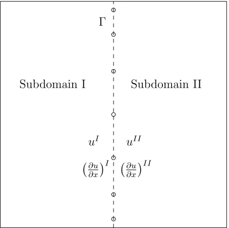
A simple domain decomposition for a rectangular domain is illustrated in Figure 1. On the interface Γ between two subdomainsI and II, one can choose unknown values in the form of a Dirichlet-Dirichlet type or a Neumann-Dirichlet type. The present work employs the Dirichlet-Dirichlet type

uI k =u

II k =u

Γ

k, k ={2,3,· · · , Ny−1}. (24)

These unknowns {uΓ

k} Ny−1

k=2 will be determined by matching the first-order normal

derivative ofu at the interface Γ

∂uk

∂x

I

=

∂uk

∂x

II

, k ={2,3,· · · , Ny−1}. (25)

Let f p denote the interior points on Γ. To form the interface system (25) (the so-called Schur complement system), one needs to compute the vectorf∂u

∂x

with each of two subdomains at f p in terms of nodal boundary values of u (i.e. e

u(bp)).

Using (15), the values of∂u/∂x along Γ are computed by

f

∂u ∂x

!

(f p)

=De(1_{(f p,bp}x) ₎u(_ebp)+De(1_{(f p,ip}x) ₎eu(ip)+el(1_{(f p}x)₎. (26)

Taking (21) into account, the second term on the right-hand side of (26) is replaced with

e

D₍(1_{f p,ip}x) ₎u_e(ip)=−De(1

x) (f p,ip)Ae−

1

(ip,ip)Ae(ip,bp)ue(bp)+De(1

x) (f p,ip)Ae−

1 (ip,ip)

eb(ip)−el(2

x) (ip) −el

(2y) (ip)

.

(27) In (26) and (27), there remain three terms, namelyel₍(1_{f p}x₎),el(2_(ipx₎)andel₍(2_ipy₎), which contain the values of

b−∂2u/∂t2 (28)

(t− is the direction tangent to a local boundary) at the interior points on the four sides of each subdomain. These values are known on the three actual boundaries, but unknown on the interface Γ. The following are two approaches proposed for the approximation of ∂2_u/∂t2 _{on Γ}

3.1.1 Approach 1

This approach uses differential collocation formulations and hence one can have

d

∂2_u ∂t2 =

d

∂2_u ∂y2 =D

2_bu=D2

where D is the differentiation matrix whose entries are explicitly known (see, e.g., [3], [4], [5]).

3.1.2 Approach 2

This approach is based on the integral collocation formulation

d

∂2_u ∂t2 =

d

∂2_u ∂y2 =Db

(2y)

      b u

∂2_u 1

∂y2

∂2_u

Ny ∂y2      = b

D(2y)

                uΓ 1 uΓ 2 · · · uΓ Ny

∂2_uΓ 1

∂y2

∂2_uΓ

Ny ∂y2                 , (30)

in which the values of ∂2_uΓ

1/∂y2 and ∂2uΓNy/∂y

2 _{are easily obtained using (1).}

For calculating the values of ∂2_u/∂t2 _{at the interior point on Γ, the first and last}

rows ofD2 in (29) and ofDb(2y) _{in (30) are removed.}

It can be seen that the two vectorsf∂u ∂x

I

(f p) and

f∂u

∂x

II

(f p) are now written in terms

of nodal boundary values of u. By substituting them into (25) and then imposing Dirichlet boundary conditions, one obtains a determinate system of equations for the interface unknown vectoruef p =

uΓ2, uΓ3,· · · , uΓNy−1

T

3.1.3 A C2 _{solution across the interface}

From the above process, i.e. (24), (25), (10) and (20), the following constraints are imposed at the interior points on the interface Γ

uI k=u

II

k , (31)

∂uk ∂x I = ∂uk ∂x II , (32)

∂2_u

k

∂x2

I

=bI k−

∂2_u

k

∂y2

I

, (33)

∂2_u

k

∂x2

II

=bIIk −

∂2_u

k

∂y2

II

, (34)

wherek = 2,3,· · · , Ny−1.

Consider (33) and (34). Approximations for∂2_u

∂y2

I

and∂2_u

∂y2

II

along the interface Γ are identical because they are based on the same information. On the other hand, one also hasbI

k=bIIk . The two equations (33) and (34) thus lead to

∂2_u

k

∂x2

I

=

∂2_u

k

∂x2

II

, k = 2,3,· · · , Ny−1. (35)

Hence, equations (31), (32) and (35) indicate that the present DD technique provides aC2 _{solution across the interface Γ.}

3.2

Multiple subdomains

The solution procedure for the case of two subdomains is now extended to the case of multiple subdomains. Special attention needs to be paid to the treatment for continuity conditions at the interior corner points.

In the case of many subdomains, this approach thus produces one unknown value at each interior corner point, and correspondingly one needs to add one additional equation to the interface system. Possible choices for this equation include

∂u ∂x L = ∂u ∂x R , (36) ∂u ∂y B = ∂u ∂y T , (37) 1 2

∂2_u ∂x2

L

+

∂2_u ∂x2 R + 1 2

∂2_u ∂y2

B

+

∂2_u ∂y2

T

=b, (38)

where L, R, B, T stand for left, right, bottom and top of the interior corner point, respectively. Among them, it can be seen that only (38) uses information from both

x− and y− directions. To investigate the effect of continuity order of the approx-imate solution at the interior corner points, (38) is chosen here. The computed solution is seen to beC2 _{continuous at the interior points on the interfaces and “C}0

continuous” at the interior corner points.

For Approach 2, there are three values (u, ∂2_u/∂x2 _{and ∂}2_u/∂y2_{) at each interior}

corner point as shown in (30). To achieve a C2 _{solution at an interior corner point,}

the basic idea here is to also consider the values of ∂2_u/∂x2 _{and ∂}2_u/∂y2 _{as two}

additional unknowns. Since the number of unknowns becomes greater (3 instead of 1), one can add the following three independent equations

∂u ∂x L = ∂u ∂x R , (39) ∂u ∂y B = ∂u ∂y T , (40)

∂2_u ∂x2 +

∂2_u

∂y2 =b, (41)

can be seen this treatment provides aC2 _{solution at the interior corner points. The}

accuracy of Approach 2 is expected to be better than that of Approach 1.

For problems with Neumann boundary conditions, a slight modification for the conversion process is required. The extra equation at a point on the actual boundary is utilized to implement a normal derivative boundary condition. Since the normal derivative∂u/∂n(n−the direction normal to the local boundary) is prescribed along the boundary, this equation does not introduce any new unknowns. The other extra equation at a point on the interface is employed as before and hence continuity of the second-order derivatives of u across the interface is maintained.

4

Numerical results

The grid size is defined as the minimum of average distances between the grid points in thex− and y−directions

h= min{Lx/(Nx−1), Ly/(Ny−1)}, (42)

whereLis the length of the side andN is the total number of points. The accuracy of a numerical solution is measured via a discrete relativeL2 error

Ne(f) =

v u u u u t

PM i=1

fi(e)−f

(a)

i

2

PM i=1

fi(e)

2 , (43)

whereM is the total number of collocation points, and f(e) _{and f}(a) _{the exact and}

4.1

Function approximation

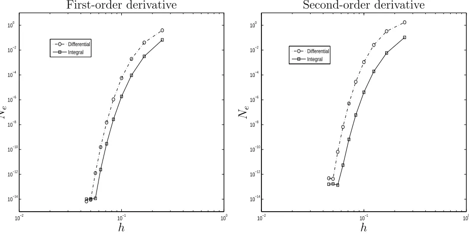
This section is concerned with a special class of function approximation. Apart from a given set of function nodal values, one also knows some nodal values of its derivatives. In this case, the use of the integral formulation can enhance the quality of the function approximation. This is demonstrated through the calculation of first-and second-order derivatives of the following function

y= sin(x), −1≤x≤1, (44)

where the values ofyat the whole set of grid points and the values ofd2_y/dx2 _{at the}

two boundary points are given. The numerical schemes used here are similar to those described in Approach 1 and Approach 2, respectively. In determining expansion coefficients, conventional differential formulations use the set of function values only, while the integral formulation takes all information into account. Results concerning

Ne(dy/dx) and Ne(d2y/dx2) are shown in Figure 2. Both formulations employ the

same sets of grid points. It can be seen that the integral formulation yields a higher degree of accuracy than the differential one.

4.2

Partial differential equations

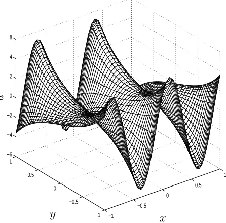
The present DD technique is verified through the solution of the following Poisson equation

defined on the square −1≤x, y ≤1, subject to Dirichlet boundary conditions

u=−sinh(2y), x=±1, (46)

u= sin(2πx) cosh(±2)−cos(2πx) sinh(±2), y=±1. (47)

The exact solution of (45)-(47) can be verified to be

u= sin(2πx) cosh(2y)−cos(2πx) sinh(2y), (48)

which is depicted in Figure 3.

The problem domain is divided into 2, 4, 9, 16, 25, 36 and 49 subdomains. For a fixed number of subdomains, various tensor product grids are employed to study the convergence behaviour of the method.

4.2.1 Comparison with conventional differential DD techniques

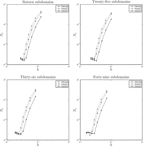
To assess the performance of the present integral DD technique, the obtained results are compared with those of conventional differential DD techniques. It is noted that conventional techniques yield only a C1 _{solution across the interfaces; the solution}

procedure used here is similar to that described in [3]. Figures 4 and 5 show plots of Ne(u) versus h. For a fixed number of subdomains, it can be seen that both

techniques yield spectral accuracy and the accuracy of Approach 1 (legend “Inte-gral(1)”) and Approach 2 (“Integral(2)”) is superior to that of the conventional one (“Differential”).

To study the influence of the C2 _{condition on the solution accuracy, the case of a}

and “Integral(2)”) are much wider than that for the single domain case (legends “Differential” and “Integral”). If one takes results obtained by the differential for-mulation as the basis, the integral forfor-mulation is seen to perform much better for the case of multiple subdomains than for the case of a single domain. It thus appears that the achievement of a C2 _{solution across the interfaces results in a significant}

improvement in accuracy.

4.2.2 Comparison of the performance of the integral DD technique

be-tween Approach 1 and Approach 2

The main difference between Approach 1 and Approach 2 is that a second-order continuity of the solution is achieved at every point on the interfaces for the latter, but only at the interior points on the interfaces for the former.

For the case of 2 subdomains, there are no interior corner points. Numerical results show that the performance of Approach 2 is similar to that of Approach 1 despite the fact that the former yields more accurate results than the latter for function approximation (Section 4.1). From Figure 4, there is no discernible difference of

Ne(u) between the two approaches.

For the case of 4 subdomains, there is only one interior corner point. The perfor-mance of Approach 2 is slightly better than that of Approach 1. However, it is still difficult to see the gap between two curves from the plot (Figure 4).

For the case of 9 subdomains and more, a number of interior corner points become noticeable. Approach 2 is found to be more accurate than Approach 1 by about two orders of magnitude.

intersec-tion points strongly affects the accuracy of the integral DD technique which is always better than differential DD techniques. Approach 2 is recommended for practical use.

5

Concluding remarks

In this paper, a domain decomposition technique which provides aC2_{, instead of the}

usual C1_{, solution for second-order elliptic problems is reported. This achievement}

of higher-order smoothness is due to satisfaction of the governing equation on the boundaries. Two approaches are proposed and studied in detail. The first approach satisfies a C2 _{condition of the solution at the interior points on the interfaces and} C0 _{at the interior corner points, while the second approach provides a C}2 _solution

at every point on the interfaces. Numerical results obtained show that

(i) both approaches outperform conventional DD techniques regarding accuracy, and

(ii) the performance of the second approach is far superior to that of the first ap-proach.

Acknowledgements

This research was supported by the Australian Research Council.

References

1. A. Quarteroni and A. Valli, Domain Decomposition Methods for Partial

Dif-ferential Equations, Clarendon Press, Oxford, 1999.

2. B.F. Smith, P.E. Bjorstad and W.D. Gropp, Domain Decomposition

Paral-lel Multilevel Methods for Elliptic Partial Differential Equations, Cambridge

3. C. Canuto, M.Y. Hussaini, A. Quarteroni and T.A. Zang, Spectral Methods in

Fluid Dynamics, Springer-Verlag, New York, 1988.

4. B. Fornberg, A Practical Guide to Pseudospectral Methods, Cambridge Uni-versity Press, Cambridge, 1998.

5. L.N. Trefethen, Spectral Methods in MATLAB, SIAM, Philadelphia, 2000.

6. N. Mai-Duy, An effective spectral collocation method for the direct solution of high-order ODEs, Communications in Numerical Methods in Engineering 22(6) (2006) 627–642.

7. N. Mai-Duy and R.I. Tanner, A spectral collocation method based on inte-grated Chebyshev polynomials for biharmonic boundary-value problems,

Jour-nal of ComputatioJour-nal and Applied Mathematics 201(1) (2007) 30–47.

8. N. Mai-Duy and T. Tran-Cong, An efficient domain-decomposition pseudo-spectral method for solving elliptic differential equations, Communications in

Numerical Methods in Engineering, accepted.

9. A. Karageorghis, A fully conforming spectral collocation scheme for second-and fourth-order problems, Computer Methods in Applied Mechanics and

En-gineering 126 (1995) 305–314.

10. A. Karageorghis, Conforming Chebyshev spectral methods for Poisson prob-lems in rectangular domains,Journal of Scientific Computing 8(2) (1993) 123– 133.

11. D. Funaro, A. Quarteroni and P. Zanolli, An iterative procedure with interface relaxation for domain decomposition methods, SIAM Journal of Numerical

Γ

Subdomain I Subdomain II

uI _uII ∂u

∂x

I _∂u ∂x

II

10−2 10−1 100

10−14

10−12

10−10

10−8

10−6

10−4

10−2

100

Differential Integral

h

Ne

First-order derivative

10−2 10−1 100

10−14

10−12

10−10

10−8

10−6

10−4

10−2

100

Differential Integral

h

Ne

Second-order derivative

−1 −0.5

0 0.5

1

−1 −0.5 0 0.5 1 −6 −4 −2 0 2 4 6

x y

u

10−2 10−1 100

10−15

10−10

10−5

100

Differential Integral

h

Ne

Single domain

10−2 10−1 100

10−15

10−10

10−5

100

Differential Integral(1) Integral(2)

h

Ne

Two subdomains

10−2 10−1 100

10−15

10−10

10−5

100

Differential Integral(1) Integral(2)

h

Ne

Four subdomains

10−2 10−1 100

10−15

10−10

10−5

100

Differential Integral(1) Integral(2)

h

Ne

Nine subdomains

Figure 4: Poisson equation. For each case, a number of tensor product grids, namely

5×5,7×7,· · · ,17×17, are employed. For the case of two subdomains, there is

no discernible difference of Ne between Integral(1) (Approach 1) and Integral(2)

10−2 10−1 100

10−15

10−10

10−5

100

Differential Integral(1) Integral(2)

h

Ne

Sixteen subdomains

10−2 10−1 100

10−15

10−10

10−5

100

Differential Integral(1) Integral(2)

h

Ne

Twenty-five subdomains

10−2 10−1 100

10−15

10−10

10−5

100

Differential Integral(1) Integral(2)

h

Ne

Thirty-six subdomains

10−2 10−1 100

10−15

10−10

10−5

100

Differential Integral(1) Integral(2)

h

Ne

Forty-nine subdomains

Figure 5: Poisson equation. For each case, a number of tensor product grids, namely