Rochester Institute of Technology
RIT Scholar Works
Theses Thesis/Dissertation Collections
12-2017
Image Down-Scaler Using the Box Filter Algorithm
Vaishnavi Parthipan
Follow this and additional works at:http://scholarworks.rit.edu/theses
This Master's Project is brought to you for free and open access by the Thesis/Dissertation Collections at RIT Scholar Works. It has been accepted for inclusion in Theses by an authorized administrator of RIT Scholar Works. For more information, please [email protected].
Recommended Citation
Image Down-Scaler Using The Box Filter Algorithm
by
Vaishnavi Parthipan
Graduate Paper
Submitted in partial fulfillment of the requirements for the degree of
Master of Science
in Electrical Engineering
Approved by:
Mr. Mark A. Indovina, Lecturer
Graduate Research Advisor, Department of Electrical and Microelectronic Engineering
Dr. Sohail A. Dianat, Professor
Department Head, Department of Electrical and Microelectronic Engineering
Department of Electrical and Microelectronic Engineering Kate Gleason College of Engineering
Rochester Institute of Technology Rochester, New York
I would like to dedicate my project work to my family members and friends who were
Declaration
I hereby declare that except where specific reference is made to the work of others, the
contents of this paper are original and have not been submitted in whole or in part for
consideration for any other degree or qualification in this, or any other University. This
paper is the result of my own work and includes nothing which is the outcome of work
done by others, except where specifically indicated in the text.
Vaishnavi Parthipan
Acknowledgements
I would like to thank my advisor, professor, Mark A. Indovina, for all of his constant
Abstract
One of the indispensable aspects of digital image processing is the requirement of varied
image resolutions. To achieve varied resolution, scaling comes into picture. Two important
applications of scaling is good pictorial quality for human interpretation and processing
of digital images for storage, transmission and for representation of autonomous machine
perception. This paper focuses on the transmission application. The size of the image if
reduced occupies less space in the communication medium thus reducing the bandwidth
requirement. And also the server space and the processing power of the image is reduced
greatly. The standard for digital television transmission over terrestrial, cable and satellite
networks is defined by Advanced Television Systems Committee (ATSC), with either 704
× 480 or 640 × 480 pixel resolutions, at 24, 30, or 60 progressive frames per second. This
paper proposes a monochrome and colored image down scaling core with memory banks
for accessing the image pixels. A 704 x 480 pixel resolution image was used. The core
has minimum complexity and was developed in Hardware Descriptive Language (HDL).
Contents
Declaration ii
Acknowledgements iii
Abstract iv
Contents v
List of Figures vii
List of Tables viii
1 Introduction 1
1.1 Organization . . . 3
2 Literature Review 4 3 Technical Overview 8 3.1 Bitmaps . . . 8
3.2 Color depth . . . 9
3.2.1 1-bit (black and white) . . . 9
3.2.2 8-bit grey . . . 9
3.2.3 24-bit RGB . . . 10
3.3 Resolution . . . 11
3.4 Aspect ratio . . . 12
4 Box Filter algorithm 13 5 Hardware Architecture 16 5.1 Register Bank Architecture . . . 16
5.1.0.1 REGISTER BANK - Horizontal input pixel register bank 16 5.1.0.2 REGISTER BANK - virtual pixel register bank . . . 18
Contents vi
5.3 Control Switch . . . 19
6 Design and Test-bench 22 6.1 Top-Level Design flow . . . 22
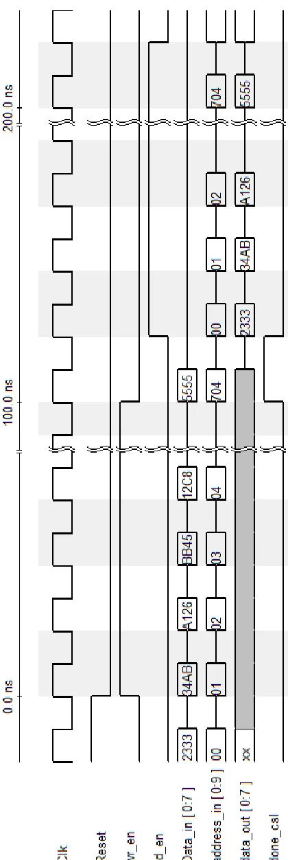
6.2 Timing diagram . . . 24
6.2.1 Register bank . . . 25
6.2.2 Filter . . . 25
6.3 Test-bench Setup . . . 25
6.4 Python Programs . . . 28
7 Result and Conclusions 29 7.1 Image Down-Scaler Module Implementation and Verification . . . 29
7.2 Implementation Results . . . 31
7.3 Conclusions . . . 34
References 35
I Image Down-Scaler Module Verilog Source Code I-1
I.1 Horizontal register bank .v file . . . I-1
I.2 Virtual register bank .v file . . . I-10
I.3 Filter: Down_scaler .v file . . . I-16
I.4 im_scaler RGB .v file . . . I-18
I.5 Horizontal register bank test-bench . . . I-24
I.6 Virtual register bank test-bench . . . I-27
I.7 Filter : Dow_scaler test bank test-bench . . . I-29
I.8 im_scaler RGB test-bench file . . . I-30
I.9 im_scaler Greyscale .v file . . . I-33
I.10 im_scaler Greyscale test-bench . . . I-39
II Python Script Files II-1
II.1 Image to bits conversion file . . . II-1
II.2 Python implementation of the Filter . . . II-2
List of Figures
3.1 8-bit gradient . . . 10
3.2 RGB color Format . . . 10
4.1 Box filter method . . . 14
5.1 Horizontal buffer . . . 17
5.2 Virtual buffer . . . 18
5.3 Filter: Pixel downscaler . . . 19
5.4 Ripple carry adder for two pixel . . . 20
5.5 Control switch . . . 21
6.1 Top-level Design . . . 23
6.2 Flow of data in the design . . . 24
6.3 Timing diagram for Register bank . . . 26
6.4 Timing diagram for filter . . . 27
7.1 Original image . . . 30
List of Tables
7.1 Area comparison of lower level blocks in 32nm Library (µm)2 . . . 31
7.2 Pre-Scan Netlist synthesis cell area (µm)2 . . . . 32
7.3 Post-Scan Netlist synthesis cell area (µm)2 . . . . 32
7.4 Pre-scan netlist synthesis Power Report . . . 33
7.5 Post-scan netlist synthesis Power Report . . . 33
7.6 Pre-scan netlist synthesis Timing Report . . . 33
Chapter 1
Introduction
Digitizing an image has many benefits in transmitting, processing, and storing the image
data [1]. Digital images are widely used in the field of consumer electronics and medical
industry. Digital television (DTV) is an advanced broadcasting technology for television
where digital image transmission and processing plays a vital role. Unlike earlier television
technology where video and audio were analog signals, DTV in contrast is used for television
signal transmission with sound channel and by digital encoding. After the evolution of
color television in 1950s, DTV marks one of the significant innovations. Digital television
provides broadcasters to offer television with better picture and sound quality along with
multiple channels of programming.
Different countries have different standards for broadcasting digital television.
Ad-vanced Television System Committee (ATSC) uses eight-level Vestigial Side-Band (8VSB)
for terrestrial broadcasting. This standard has been adopted by six countries: United
States, Canada, Mexico, South Korea, Dominican Republic and Honduras. Multiple
chan-nel transmission takes place in a single bandwidth. Due to the requirement of multi-chanchan-nel
2
the bandwidth for video communication is minimal and always in need for more. The never
ending growth in the area of digital communication fueled many communication algorithms
to meet the need of bandwidth. One such communication algorithm is scaling of images,
which helps to reduce the size before transmission.
ATSC uses 640"480-pixel or 702"480-pixel resolution for transmission over terrestrial
and satellite networks. Digital terrestrial broadcasting can be designed to work with
roof-top antennas but also with small antennas built into portable devices and for mobile
reception [2]. To reduce the bit rate while transmitting, the resolution of the images in
the video frames are reduced. At receiving end the image is interpolated by pixels to
reconstruct image to the size of destination display monitor. This paper concentrates on
the challenging and significant facet i.e., down scaling of image to address the bandwidth
need. The basic concept of image scaling is to re-sample a two-dimensional function on a
new sampling grid. There are various down-scaling algorithm available, out of which this
paper implements box filter for various reasons. Box filter algorithm is not for the images
perceived for visual content. It is mainly for the transmission purpose.
The box filter is a simple filter that can be efficiently calculated by storing partial
sums [3]. Another reason for choosing box-filter is the computational complexity. The
computational complexity is very low compared to other filters such as cubical and
bi-linear filters used for down-scaling. If implemented in an Application Specific Integrated
Circuit (ASIC), or a Field Programmable Gate Array (FPGA), the number of logic gates
required will be very less, but in contrast it needs more on chip memory register banks for
storage of the partial sum. The use of on-chip memories nowadays are expected to increase
continuously based on the future generation high performance and portable devices [4]. An
FPGA is an integrated circuit, which is configured after manufacturing using a Hardware
1.1 Organization 3
memory for storage of original pixels and the intermediate partial sum pixels. The down
scaling core is coded in HDL (Hardware Descriptive Language) and has been benchmarked
in a ASIC core module targeting 32 nm, 65nm, 90nm and 180nm technologies.
1.1 Organization
The organization of this paper is as follows: Chapter 2 discusses about the comparison
between different algorithm used for down-scaling, Chapter 3 gives an insight into the
Technical Concepts related to digital image down-scaling and Chapter 4 explains the
Al-gorithm used in this paper. Next, Chapter 5 explains the Hardware Implementation of
the algorithm, Chapter 6 discusses about the Design Flow and Test-bench and the final
Chapter 2
Literature Review
There are three main methods used for image down-scaling: bi-linear, bi-cubical and
Near-est neighbor algorithm. This section deals with these different methods and why box filter
is a better choice for image down-scaling.
One of the widely used algorithms for down-scaling is the cubical algorithm.
Bi-cubical interpolation is used in a two dimensional grid for interpolating pixels. This is
derived from the cubic interpolation. As the name depicts, the ’Bi’ in this algorithm
refers to computing two 1 dimension operations: vertical and horizontal computation. This
algorithm is used is for most of images, assuming the image is size not to small, or that this
image is not highly detailed, or if the edges of the image are to be kept smooth. Moreover
the contrast and artifacts are increased using the bi-cubic algorithm. The operation of
bi-cubic convolution requires the calculation of 16 weighted coefficients generated from
5
obtained from the Equation2.1.
c=
1−2|d|2+|d|3 , 0≤ |d|<1
4−8|d|+ 5|d|2 − |d|3 , 1≤ |d|<2
0 , 2≤ |d|
(2.1)
Then four virtual pixel(V0, V1, V2andV3) are calculated by either vertical or horizontal
interpolation as shown in Equation2.2.
3
X
i=0
Ai,j " vci (2.2)
where vciis the vertical co-efficient of one of the (4 " 4) pixels Ai,j.
As described in [5], the operation of this filter in addition to the calculation of the
weighted co-efficient, also requires the co-ordinates of the pixel. The number of adders
and multipliers used for implementing the co-efficient calculation are high. To achieve
bi-cubical interpolation with good results, a high number of resources are required. There
is additional hardware to satisfy the need of the complexity such as the Pixel co-ordinate
generator, horizontal and vertical pixel generator, and a virtual pixel buffer. The vertical
pixel generator stores the calculated intermediate pixel in the virtual pixel buffer. Since
most of the image doesn’t come with inbuilt memory, the number of memory reads and
writes are high. Memory reads are costly in certain cases. This is avoided in the proposed
box filter with register banks to store pixel values. If a scale factor of 2×2 is used with
bicubic interpolation, the hardware implementation of an image expansion method can be
significantly simplified [6].
Bi-cubic interpolation is a robust technique compared with other techniques such as the
6
less resources and are more feasible for implementation in sequential processors [8]. Due
to less complexitybox filter is faster compared to bi-cubic filter. Note that the bi-cubic
interpolation method is somewhat complicated as compared to bi-linear interpolation [9].
In contrast to the bi-cubic algorithm which takes 16 pixels (4"4) , the bi-linear algorithm
uses only 4 pixels (2 " 2) in account. Bi-linear is extension of linear interpolation. The
main motive is to perform linear interpolation in one direction and then repeat the same
in another direction. This method reduces the contrast of the image, and never produces
a satisfying image, combining a fuzzy overall look with jagged edges and motion artifacts
[10]. This algorithm takes the weighted average of the four closest pixels, and maps it to
the specified output co-ordinates. The speed at which the output pixels are calculated is
low compared to other techniques [11]. Apart from having the slow calculation unit, the
technique described in this paper has an extra graphical processing unit to accelerate the
process. The calculation time was faster but only after giving away resources. One other
disadvantage of using the bi-linear algorithm is that its more efficient for images with lesser
pixels. Since it computes the weighted average of (2 " 2) pixels, the amount of time it
would take to compute the entire image would be significantly high. The weight on each
of the 4 pixel values is based on the computed pixel’s distance (in 2D space) from each of
the known points.
Let us consider four pixelsR1,1,R1,2, R2,1 and R2,2 in a (x, y) co-ordinate system. Now
let Q1 be weighted average ofR1,1 and R2,1. Similarly Q2 be weighted average ofR2,1 and
R2,2. First, the Q1and Q2 values are calculated using the Equation 2.3 and 2.4. Here x1,
x2 ,y1 and y2 represent the position in the co-ordinate system.
7
Q2 = ((x2–x)/(x2–x1))∗R1,2+ ((x–x1)/(x2–x1))∗R2,2 (2.4)
Second, after the calculation of Q1 and Q2, the down-scaled pixel valueP is calculated
by the Equation2.5.
P = ((y2–y)/(y2–y1))∗Q1 + ((y–y1)/(y2–y1))∗Q2 (2.5)
So if we take a closer look at Equation 2.3 and 2.4, we see they deal with the x-axis
of the co-ordinate system. Thus, the interpolation happens in one direction and then the
interpolation is repeated in the other direction y, as given in Equation2.5. The paper [12]
uses the bi-linear algorithm and requires eight multiplications, three additions and four
subtractions.
One weakness of bi-linear, bi-cubic and related algorithms is that they sample a specific
number of pixels. When down scaling below a certain threshold, such as more than twice for
all bi-sampling algorithms, the algorithms will sample non-adjacent pixels, which results in
losing data and causes rough results. And these traditional downscaling algorithms mainly
address the aliasing problem [13].The trivial solution to this issue is box sampling, which
is to consider the target pixel a box on the original image, and sample all pixels inside the
box. This ensures that all input pixels contribute to the output. The major weakness of
this algorithm is that it is hard to optimize. But these two algorithms are useful when high
quality image is required. But one of the main drawback of such algorithm is the amount
of resources used. Where as other techniques are simpler and need less resources. The
common thing among all the three algorithms is after certain input latency, the pixel value
is calculated at the data rate. Area averaging or box filter on the other hand is simple,
Chapter 3
Technical Overview
This chapter gives an elementary introduction to bit-mapping, aspect ratio and resolution
aspect of an image.
3.1 Bitmaps
Bitmaps are defined as a rectangular mesh of cells called pixels. Each pixel in an image
carries the color of the designated co-ordinate in a image [14]. The value of the pixel in
each cell gives the color value. Bit maps are defined by only two characteristics namely
the number of pixels and the information content of the pixel (color depth). Apart from
the number of pixel and pixel content (two parameters), there are other parameters which
are derived from these two fundamental parameters.
The layout of the bitmap is generally aligned horizontally and vertically. In most cases
3.2 Color depth 9
3.2 Color depth
Each pixel contains information about the color of the image. This information content
is called color depth. Color depth refers to the number of bits used to represent color
information of either a single pixel or the number of bits of each color component of a
single pixel depending on the image format. Images with higher bit depths can encode
more shades or colors since there are more combinations of 0’s and 1’s available [15].
3.2.1 1-bit (black and white)
This is the smallest possible content that can be held by a pixel [14]. The bit 0 is represented
for white and 1 describes the black in that pixel. The resulting bitmap is called monochrome
or black and white image. Since there are only two values, the pixel can be used to represent
0 as black and 1 as white also.
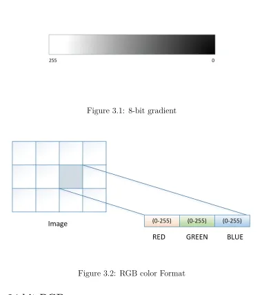
3.2.2 8-bit grey
In this case each pixel takes 8 bit or 1 byte of data to store the color value. Then the values
of the pixels will be from 0 to 255. If these different values are mapped on to a ramp of
1 to 8 bit, then these are called as greyscale images shown in Fig 3.1. 0 is normally black
and 255 white. The in-between values are the grey levels, for example, in a linear scale 127
would be a 50% grey level.
In any particular application the range of grey values can be anything, and it is most
common to map the levels 0-255 onto a 0-1 scale; some programs will map to a 0-65535
scale. Digital images requires, at a minimum an 8-bit per pixel where 256 discrete levels
3.2 Color depth 10
Figure 3.1: 8-bit gradient
Figure 3.2: RGB color Format
3.2.3 24-bit RGB
The 24-bit RGB format is used to represent a colored image. Here 8 bits are allocated to
each red, green, and blue component of a pixel. In each component the value of 0 refers
to no contribution of that color, 255 refers to fully saturated contribution of that color.
Since each component has 256 different states there are a total of 16777216 possible colors
as shown in Fig. 3.2.
[image:20.612.115.495.100.527.2] [image:20.612.132.481.302.451.2]3.3 Resolution 11
colored image. The greyscale image is represented in a 8-bit format and the colored image
is represented in 24-bit format.
3.3 Resolution
Pixels themselves don’t have a dimension, so the resolution attribute of bitmap comes in
the picture for visually viewing or printing. Resolution is normally specified in pixels per
inch but could be in terms of any other unit of measure. Most printing processes retain
the Pixels Per Inch (PPI) or Dots Per Inch (DPI) units for historical reasons. In digital
printing world, DPI is defines the amount of pixels that can be accommodated in line or
area within a span of 1 inch. PPI has similar definition to DPI, but here the amount of
pixel referred is in a digital image. The resolution may be specified as two numbers, the
horizontal and vertical resolution.
The information in the bitmap content is different from the perspective of resolution of
that image, given a constant color depth then the information content between different
bitmaps is only related to the number of pixels vertically and horizontally. The quality of
the image, when printed or displayed as digital image hugely depends on the resolution.
In-order to modify the overall image size the resolution of the image is changed.
As an example consider one bitmap which is 200 pixels horizontally and 100 pixels
vertically. If this bitmap was printed at a resolution of 100 DPI, then it would measure 2
inches by 1 inch. If however the same bitmap was printed at 200 DPI then it would only
3.4 Aspect ratio 12
3.4 Aspect ratio
The ratio of width to the height of an image is called aspect ratio. It is usually represented
by two numbers with a colon separation, like 4:3. If there are three different images say, 4
inches wide and 3 inches high, 4 mm wide and 3 mm high. All have the same aspect ratio.
This means the size of the image does not concern the aspect ratio. The international
standard aspect ratio for digital television is 16:9. This aspect ratio one of the wide screen
ratio that is supported by the [1]. Pixels are usually considered as a square, all though
they have other aspect ratios.
The image used in this paper is (704 ×480) pixels, which is 704 pixel horizontally
and 480 pixels vertically. Downsizing image and video content of resolutions 704 " 480,
640×480 and 320×240 are of interest as many mobile devices have displays with such
resolutions [17]. These resolutions translate to downsizing factors of 4/9 × 3/8, 4/9 × 1/3
Chapter 4
Box Filter algorithm
A box filter, also known as “moving average”, is a simple linear filter with a square (or
rectangular) kernel and all kernel coefficients equal and it is the quickest filter algorithm,
but it lacks smoothness of a Gaussian filter [18]. The number of logic gates required for
this algorithm is less, however in this paper register banks that are required to store the
partial sums increase the area required. These register banks are reused when compared to
the naive implementation where partial sums are not stored. Every time a partial sum is
necessary, it is recalculated on demand in such implementation. Higher resolution images
require more register banks, since the partial sum corresponds to the size of image width.
The computational complexity of image filtering depends on the complexity and size of
the filter. There are two different approaches for this filter : integral image algorithm [19]
and summed area algorithm [20]. In this paper we are using the summed area algorithm.
Before starting the explanation of the filter method, lets go through some terminologies.
Source image is the original image before scaling up/down. Target image refers to the scaled
image. The region of the target pixel in the source that are being calculated currently is
14
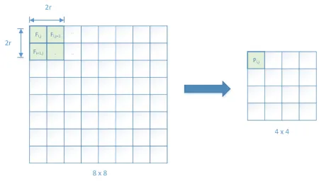
Figure 4.1: Box filter method
Box filter is a simplest linear filter. Each pixel calculated is the average of the pixel
values in a square (filter window) centered at that pixel. The difference between box filter
and other linear filter is that the rest of them use a weighted average. The calculation the
target pixel is by moving the averaging window either horizontally or vertically. In this
paper the window is moved horizontally as shown in Fig.4.1.
Let P be the pixel value of the targeted pixel. From Fig.4.1 it can be noted that the
window size is 2 " 2. Here the window size is an even number of rows and columns i.e,
2r " 2r, where r is the window radius. It is also possible to have odd number of rows
and columns. In that case the window size will be (2r + 1) " (2r+ 1). Let Fi,j, for
[image:24.612.82.532.101.364.2]15
independent of a filter radius [21]. The formula for the targeted pixel value is given by
Pi,j = m
X
k=0 m
X
l=0
wk,l Fi+k,j+l (4.1)
for i, j = (m+ 1), ....(n−m).
Let m = 1, then the window over which the averaging is carried out is 2 " 2 and Pi,jis
given by
Pi,j = W0,0 Fi,j + W0,1 Fi,j+1 + W1,0 Fi+1,j + W1,1 Fi+1,j+1 (4.2)
Here for the box filter the weights distributed for all the four pixels are equal. This
then becomes the average of the four pixels.
P = 1
(2r)2 Fi,j + Fi,j+1 + Fi+1,j + Fi+1,j+1 (4.3)
The implementation of the filter in this paper has 4 register banks to store the original
pixels and 2 register bank to store the partial sum of the pixels. One advantage of this
implementation is there is no memory access. As implemented in this paper, the resolution
is constant, thus the register banks to store the original pixel before calculation and to store
Chapter 5
Hardware Architecture
Detailed information about each block of the image scaler is explained here.
5.1 Register Bank Architecture
Considering the width of the image, the size of the register bank is decided. Here there
are two different register banks, one for storing the source pixels, i.e., input pixels, and the
second is used to store the intermediate pixels or virtual pixels that are used for further
down-scaling.
Let us discuss the two different register banks used here.
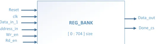
5.1.0.1 REGISTER BANK - Horizontal input pixel register bank
This register bank is used to store the pixel value in horizontal manner. The image is
read row by row. Each row contains 704 pixels. Therefore, there are 704 unpacked 8-bit
width register blocks for greyscale images, and 24-bit wide registers for colored images.
5.1 Register Bank Architecture 17
Figure 5.1: Horizontal buffer
register bank. This address is carried throughout the design, for storage of virtual pixels
as well as for the output pixel. The control signals wr_en and rd_en are active HIGH
signals. Apart from the write and read enabling operations, these signals are also used as
to synchronize operations between register banks. Fig. 5.1 shows the horizontal register
bank block diagram.
These control signal are driven by a switch that decides which register bank needs to
be written with input pixel values and which register bank needs to be read. More details
about the Control signal is given in the section5.3. There are total of four horizontal input
pixel buffers. A pair of register banks is used for the storage of the consecutive rows at a
given HIGH wr_en. Once these two registers are filled, the corresponding rd_en stroke is
enabled to read those registers. The pair of registers are written and read one after the
other. Total of 704 clock cycles is required to store two rows of pixels in a pair of register
banks. Once the register banks are filled, a Done_cs signal is asserted to indicate that the
entire register is filled with a row of pixels.
Now coming to the output part of the register bank, if the control signal toggles to
[image:27.612.177.442.141.215.2]5.2 Filter : Pixel down-scaler 18
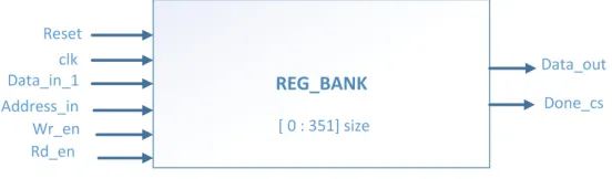
Figure 5.2: Virtual buffer
input. Thus, there is simultaneous read and write enabled in the block.
5.1.0.2 REGISTER BANK - virtual pixel register bank
These are similar to horizontal register banks but the size of number of registers varies.
The number of registers are half the number of registers used in horizontal buffers. When
the down-scaler processes each pair of horizontal register banks, it filters 2 " 2 pixels
producing 352 pixels. That is the reason for half the number of registers used in virtual
register banks. The virtual register bank block diagram is shown in the Fig. 5.2. The
address_in for the virtual register bank comes from the down-scaler. The wr_en and
rd_en signals are from the control block.
If the pixels stored in the virtual register banks are collected, they will produce an
image of size 352 " 240 pixels.
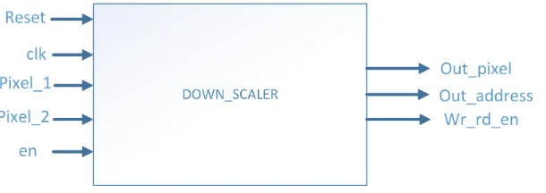
5.2 Filter : Pixel down-scaler
This block is used to downscale the input pixels. It takes two clock cycles to produce
the average of four pixels. This implementation is similar to the winscale algorithm [7]
where the filter window frame moves over the pixels that are to be averaged. But here
there is no concept of filter window, wherein here one pixel from each of the horizontal
[image:28.612.169.445.102.183.2]5.3 Control Switch 19
Figure 5.3: Filter: Pixel downscaler
adds. Once addition of four pixels are done, the filter then shifts the total sum to produce
a partial sum. The output produced is every other clock cycle. Meaning it takes two clock
cycle to produce the output. This filter apart from averaging also generates the output
address to store these pixels. This address is send to the virtual register bank for storage
of intermediate pixel. Pixel down-scaler block diagram is shown in the Fig. 5.3.
The input to the filter is from two horizontal register bank, so there are two filter for
the four horizontal register banks. And there is one filter for the two virtual register banks.
The net result is to down-scale sixteen pixels to have a resolution of 176 " 120 pixels is
achieved by a total of three filters.
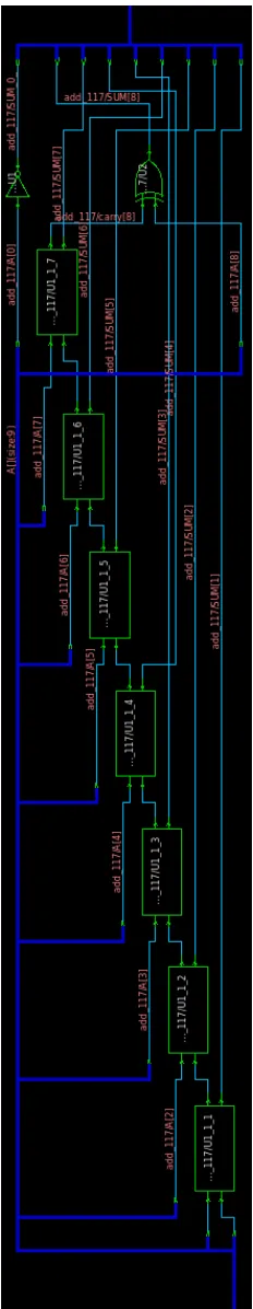
The enable signal is triggered from the test-bench, when high the two pixel that are
read will be added. The addition of the two pixels is synthesized as ripple carry adder.
These ripple carry adders are made up of half adders and full adders. The Fig. 5.4 shows
the ripple carry adder used to add the two incoming pixels.
5.3 Control Switch
Fig. 5.5shows the control switch block. The control switch produces the wr_en and rd_en
signals using two multiplexers that select which write or read signal needs to enabled, such
[image:29.612.158.463.101.209.2]5.3 Control Switch 20
[image:30.612.248.364.99.697.2]5.3 Control Switch 21
Figure 5.5: Control switch
all the write and read signals across the Image Down-Scaler module. The select signal, sel,
enables which read and write signals need to be executed. The select signal comes from
the test-bench. There are total of four wr_en signal lines, one for each horizontal register
block. This same wr_en signal is given to the virtual register bank, but wr_en are active
low for virtual register banks. In that way once the horizontal register banks fills with the
wr_en at active high, then when the wr_en goes low it triggers the virtual register bank
to write the intermediate pixel values. Similarly there are four rd_en signals that are used
[image:31.612.185.425.98.301.2]Chapter 6
Design and Test-bench
This section presents the top level design flow and the test-bench used for design
verifica-tion.
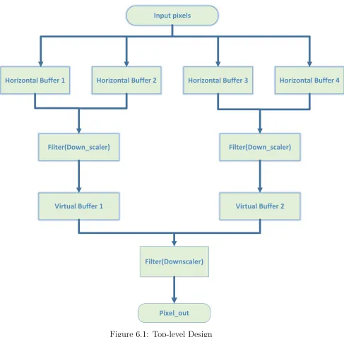
6.1 Top-Level Design flow
The top level design of the Image Down-Scaler module is shown in the Fig. 6.1.
As shown in the design two rows of pixel starting from the first row is given to the first
and second horizontal register bank. Once they are filled, the next set of registers (3 &
4) are fed with rows from the test-bench, and the rd_en signal is generated for the 1st &
2nd registers by the control signal block. The Fig. 6.2 shows the flow of data throughout
the design. When the second set of registers are being written, the filter starts reading the
first set of register values and starts computing the output, which is average of four pixel.
In Fig. 6.2 the writing into register is shown in green and the filter operation done before
virtual register is shown in red color. And when again the first set of registers are being
6.1 Top-Level Design flow 23
[image:33.612.78.565.155.632.2]6.2 Timing diagram 24
Figure 6.2: Flow of data in the design
These filtered values are store in virtual buffers 1 and 2 as shown in Fig. 6.1. When
both the virtual register banks are filled, the final down-scaler is enabled, this filters out
the last stage pixels. This is shown in purple color in Fig. 6.2.
Virtual buffer will store exactly half the pixel values compared to the horizontal buffer.
Now the filter following the virtual buffer receives input from the previous filter and stores
those values as they are computed. Once both the virtual buffer gets filled, the output is
generated by further averaging of the virtual pixels.
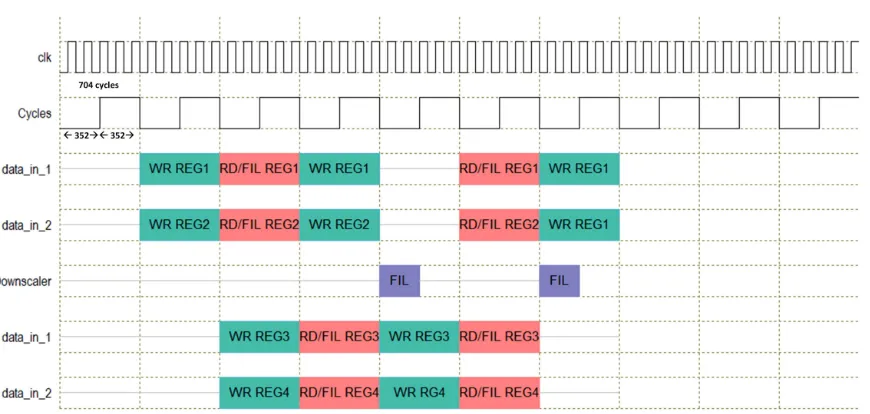
6.2 Timing diagram
The timing diagram explains the number of clock cycles each block takes for the
compu-tation. The Image Down-Scaler module is designed in such a way that it has to wait a
[image:34.612.93.528.101.308.2]6.3 Test-bench Setup 25
6.2.1 Register bank
Fig. 6.3 shows the timing diagram for the horizontal register bank and virtual register
bank. Since they are similar in operation this single timing diagram would explain the
working of both the register banks.
6.2.2 Filter
Fig.6.4 explains the timing diagram for the filter operation.
6.3 Test-bench Setup
The manipulation of the pixel value is in bits. The section gives detailed information about
the image to bits conversion, and vise-versa.
There are separate test-bench’s for verification of each lower level module. Apart from
the low level testing, there is a test-bench at the top level, which is setup in such a way
that it reads the pixel values in rows from a text file generated by a python script used to
convert images; details of this script are found in section 6.4. $readmemb is used to read
the binary pixel values from the text file. The text file is read at the start of the simulation
to initialize the data set register. Then a each clock edge a pixel is fed into the top level
module. Apart from the pixel value, the test-bench generates addresses ranging between
0-703. This address is generated in a loop, since they are a series of consecutive numbers.
The test-bench drives the data_in pixel and its corresponding address and the select
signal is driven every 704 cycles for the generating internal control signals. The full Image
6.3 Test-bench Setup 26
[image:36.612.203.413.94.720.2]6.3 Test-bench Setup 27
[image:37.612.218.397.150.612.2]6.4 Python Programs 28
6.4 Python Programs
There are three Python programs used in this project.
• The first one generates the bits from the image. Each pixel value is converted into
ASCII bit representation and stored in a text file. One single line represents the
value of single pixel. The text file is generated in this way so that it will be easy for
the $readmemb to store each pixel value in a data set register.
• The second one is used to convert the bits to an image. The collected output pixel
from the test-bench is read by this python script and converts it into image.
• Third one is the implementation of the box filter algorithm as a model for checking
operation of the hardware.
All the Python programs are given in Appendix II. Image pixel data are read and written
in Python by importing the Python Imaging Library (PIL) package. PIL adds the image
processing capability to the Python interpreter [22]. It has a powerful image processing
features and it also supports various image formats. The core image library is designed for
fast access to data stored in a few basic pixel formats. It should provide a solid foundation
Chapter 7
Result and Conclusions
7.1 Image Down-Scaler Module Implementation and
Verification
The Image Down-Scaler module is written in the Verilog Hardware Description Language
(HDL) designed at the Register Transfer Level (RTL). The lower and higher level modules
are synthesized using Synopsis Design Compiler with 32 nm, 65 nm, 90 nm and 180 nm
technology node from TMSC. The synthesis step is what transforms the RTL into a gate
level netlist, which is a physical description of the hardware consisting of logic gates,
standard cells, and their connections [23]. The synthesis is performed by inserting scan
chains through out the core, i.e., Design for Testability synthesis. The results of these
synthesis are reported in the below section7.2. The clock frequency used here is 250M Hz.
Before synthesis, the Image Down-Scaler module was simulated using the Cadence
Incisive Simulator. The SimVision Debug environment by Cadence helps to analyze the
design and test-bench in the verification process. After verifying the Image Down-Scaler
7.1 Image Down-Scaler Module Implementation and Verification 30
Figure 7.1: Original image
Figure 7.2: Downscaled to 352 " 240 image
using Synopsis synthesis tools. Once synthesized successfully, the resulting netlist was
simulated and verified. Though the code is successfully simulated and synthesized, it isn’t
pipe-lined to output the data every clock cycle. And the implementation can be more
effectively optimized by pipe-lining the Image Down-Scaler module completely. And the
image that is test does not render the output as expected. But the first level of down
scaling works where 704 " 480 is downscaled to 352 " 240 . The Fig. 7.1 shows
the original RGB color image, and the Fig. 7.2 shows the single stage downscaled image.
But the algorithm implemented in the software produces the image down scaling result as
[image:40.612.204.409.102.242.2] [image:40.612.235.377.271.373.2]7.2 Implementation Results 31
7.2 Implementation Results
This section gives the results for area, power, and timing for the four different technologies
mentioned in the section 7.1. The area distribution report results for the pre-scan netlist
are shown in Table 7.2 and for the post-scan netlist in Table 7.3. The pre-scan and
post-scan netlist are very similar. The main difference is due to the insertion of post-scan logic for
testing. Inserting scan logic changes the functionality of the design [24], hence there are
two different reports. Table7.4 shows the power report, as technology migrates to smaller
geometry leakage contribution to total power consumption increases faster than dynamic
power, indicating that leakage will be a major contributor to overall power consumption
[25].
For additional details, area of lower level block synthesized in 32 nm library technology
are given in the Table 7.1. This shows that the major amount of area is covered by the
register banks.
Table 7.1: Area comparison of lower level blocks in 32nm Library (µm)2
Technology
Node
Down-Scaler Horizontal register bank Virtual register bank
Combinational
Area
1403 615257 307296
Non-Combinational
Area
2601 1182006 591876
7.2 Implementation Results 32
Table 7.2: Pre-Scan Netlist synthesis cell area (µm)2
Technology
Node
im_scaler_32nm im_scaler_65nm im_scaler_90nm im_scaler_180nm
Combinational
Area
421722 157357 1908711 3076108
Non-Combinational
Area
603247 925288 3203283 5921817
Total Area 1024952 1082646 7108555 8997925
Table 7.3: Post-Scan Netlist synthesis cell area (µm)2
Technology
Node
im_scaler_32nm im_scaler_65nm im_scaler_90nm im_scaler_180nm
Combinational
Area
421722 157146 1908711 3071597
Non-Combinational
Area
775604 868562 3203283 7049836
7.2 Implementation Results 33
Table 7.4: Pre-scan netlist synthesis Power Report
Technology Node Internal Power Switching Power Dynamic Power Leakage Power
im_scaler_32nm 28.40mW 405.90µW 28.81mW 117.25mW
im_scaler_65nm 41.80mW 780.09µW 42.55mW 33.626µW
im_scaler_90nm 329.12mW 1.816mW 2.146mW 18.06mW
im_scaler_180nm 280.15mW 13.68mW 293.83mW 35.072µW
Table 7.5: Post-scan netlist synthesis Power Report
Technology Node Internal Power Switching Power Dynamic Power Leakage Power
im_scaler_32nm 23.40mW 405.90µW 24.29mW 128.22mW
im_scaler_65nm 45.96mW 804.63µW 46.77mW 31.79µW
im_scaler_90nm 4.14mW 3.54mW 7.68mW 22.09mW
im_scaler_180nm 320.70mW 12.84mW 333.55mW 40.33µW
Table 7.6: Pre-scan netlist synthesis Timing Report
Technology
Node
Arrival
Time (ns)
Slack (ns)
im_scaler_32nm 10.64 8.98
im_scaler_65nm 3.08 16.59
im_scaler_90nm 10.64 8.98
7.3 Conclusions 34
Table 7.7: Post-scan netlist synthesis Timing Report
Technology
Node
Arrival
Time (ns)
Slack (ns)
im_scaler_32nm 7.20 12.51
im_scaler_65nm 3.08 16.51
im_scaler_90nm 10.60 9.02
im_scaler_180nm 10.62 9.02
7.3 Conclusions
Thus, an Image Down-Scaler module with less computational complexity is implemented
in Verilog HDL. This core is synthesized with register banks to hold the pixel values, which
reduces the number of memory read and writes if the pixels were accessed from an external
memory. There is an increase in the area of this design because of the implementation of
the register banks. Note that the Image Down-Scaler module is not completely pipe-lined.
The data is output at certain intervals of time. Future work would be to fully pipe-line
References
[1] M. Petrou and C. Petrou, Image Processing : The Fundamentals. WILEY, 2010.
[2] C. Dosch, D. Hemingway, and W. Sami, Eds., Handbook on Digital Terrestrial
Tele-vision Broadcasti ng Networks and Systems Implementati. ITU, 2016.
[3] S. Wang and T. Maruyama, “An implementation method of box filter on fpga,”Field
Programmable Logic and Applications (FPL), 2016 26th International Conference,
Aug. 2016. [Online]. Available: 10.1109/FPL.2016.7577364
[4] S.M.Mehzabeen and I.Manju, “Efficient optimization of fpga on-chip memory for
im-age processing algorithm,”International Journal of Recent Technology and
Engineer-ing (IJRTE), vol. 2, May 2013.
[5] C. chi Lin, M. hwa Sheu, H. keng Chiang, C. Liaw, and Z. chuan Wu, “The
efficient vlsi design of bi-cubic convolution interpolation for digital image processing,”
Circuits and Systems, 2008. ISCAS 2008. IEEE International Symposium, May 2008.
[Online]. Available: 10.1109/ISCAS.2008.4541459
[6] A. Rangsikunpum, E. Leelarasmee, and S. Pumrin, “A design of sign video image
Engineering/Elec-References 36
tronics, Computer, Telecommunications and Information Technology (ECTI-CON), 2017 14th International Conference on, Jun. 2017.
[7] C.-H. Kim, S.-M. Seong, J.-A. Lee, and L.-S. Kim, “Winscale: an image-scaling
al-gorithm using an area pixel model,” IEEE Transactions on Circuits and Systems for
Video Technology, vol. 13, no. 6, pp. 549–553, June 2003.
[8] M. A. Nuno-Maganda and M. O. Arias-Estrada, “Real-time fpga-based architecture
for bicubic interpolation: An application for digital image scaling,” Reconfigurable
Computing and FPGAs, 2005. ReConFig 2005. International Conference, Feb. 2005.
[9] P. R. Rajarapollu and V. R. Mankar, “Bicubic interpolation algorithm implementation
for image appearance enhancement,” International Journal of Computer Science
And Technology, Jun. 2017. [Online]. Available: http://www.ijcst.com/vol8/8.2/
4-prachi-r-rajarapollu.pdf
[10] E. Callway, “Video scaling : Time to banish bilinear!” Hollywood, CA, USA, Oct.
2011.
[11] Y. Sa, “Improved bilinear interpolation method for image fast processing,”Intelligent
Computation Technology and Automation (ICICTA), 2014 7th International Conference, Oct. 2014. [Online]. Available: 10.1109/ICICTA.2014.82
[12] M. K. Daniel, V. A. Sophia, and C. J. Moses, “A comparative analysis of bilinear
based scalar algorithms,” IEEE, Mar. 2014.
[13] S. H. Junjie Liu, “L0-regularized image downscaling,” IEEE TRANSACTIONS ON
IMAGE PROCESSING, vol. 27, Mar. 2018. [Online]. Available: 10.1109/TIP.2017.
References 37
[14] P. Bourke, “A beginners guide to bitmaps,” renderings and models by Peter
Diprose and Bill Rattenbury Original November 1993. [Online]. Available:
http://paulbourke.net/dataformats/bitmaps/
[15] “A learning community for photographers,” Cambridge in color. [Online]. Available:
http://www.cambridgeincolour.com/tutorials/bit-depth.htm
[16] L. Walking, “Intoduction to digital resolution,” 2011. [Online]. Available: https:
//www.ala.org.au/wp-content/uploads/2011/10/Introducton-to-Resolution.pdf
[17] E.-L. Tan, W.-S. Gan, and S. Mitra, “Fast arbitrary resizing of images in the discrete
cosine transform domain,” IET sponsored by Institution of Engineering and
Technol-ogy, Feb. 2011.
[18] L. Alexey, “Tips & tricks: Fast image filtering algorithms,” in GraphiCon’2007, 2007.
[19] P. Viola and M. Jones, “Rapid object detection using a boosted cascade of simple
features,” Computer Vision and Pattern Recognition, 2001. CVPR 2001. Proceedings
of the 2001 IEEE Computer Society Conference, Dec. 2003.
[20] F. C. Crow, “Summed-area tables for texture mapping,” in Proc. ACM SIGGRAPH,
1984.
[21] R. Chandel and G. Gupta, “Image filtering algorithms and techniques: A review,”
International Journal of Advanced Research in Computer Science and Software Engineering, Oct. 2013. [Online]. Available: https://pdfs.semanticscholar.org/acc5/
3ba7ec21ff7eab60baf9506747c181012d6f.pdf
[22] C. Alex,Pillow (PIL Fork) Documentation. Fredrik Lundh and Contributors, 2015.
References 38
[23] S. L. Harris and D. M. Harris.,Digital Design and Computer Architecture, A. Edition,
Ed. Morgan Kaufmann, 2016.
[24] P. Rashinkar, P. Paterson, and L. Singh, SYSTEM-ON-A-CHIP VERIFICATION :
Methodology and Techniques, G. Martin and L. Rosenberg, Eds. KLUWER
ACADEMIC PUBLISHERS, 2002. [Online]. Available: http://www.ebooks.
kluweronline.com/
[25] P. Deepa and C. Vasanthanayaki, “Fpga based efficient on-chip memory for image
Appendix I
Image Down-Scaler Module Verilog
Source Code
I.1 Horizontal register bank .v file
1
2 module REG_BANK #(parameter width = 2 3 )
3 (
4 input r e s e t , 5 input c l k ,
6 input [width: 0 ]data_in, 7 input [ 9 : 0 ]a d d r e s s _ i n , 8 input wr_en,
9 input rd_en,
10 input test_mode , // DFT t e s t mode c o n t r o l
s i g n a l
I.1 Horizontal register bank .v file I-2
18 output scan_out1, // DFT scan chain output 1 19 output scan_out2, // DFT scan chain output 2 20 output scan_out3, // DFT scan chain output 3 21 output scan_out4, // DFT scan chain output 4 22 output reg done_cs,
23 output reg [width: 0 ] data_out
24 ) ;
25 reg [width: 0 ]reg_bank[ 0 : 7 0 3 ] ;
26 always@(posedge c l k or posedge r e s e t) 27 begin
28 i f(r e s e t)
29 begin
30 reg_bank[ 0 ] <= 0 ;reg_bank[ 1 ] <= 0 ;reg_bank[ 2 ] <= 0 ;reg_bank[ 3 ] <= 0 ;reg_bank[ 4 ] <= 0 ;reg_bank
[ 5 ] <= 0 ;reg_bank[ 6 ] <= 0 ;reg_bank[ 7 ] <= 0 ;
reg_bank[ 8 ] <= 0 ;reg_bank[ 9 ] <= 0 ;reg_bank[ 1 0 ] <= 0 ;reg_bank[ 1 1 ] <= 0 ;
31 reg_bank[ 1 2 ] <= 0 ;reg_bank[ 1 3 ] <= 0 ;reg_bank[ 1 4 ] <= 0 ;reg_bank[ 1 5 ] <= 0 ;reg_bank[ 1 6 ] <= 0 ;
reg_bank[ 1 7 ] <= 0 ;reg_bank[ 1 8 ] <= 0 ;reg_bank
[ 1 9 ] <= 0 ;reg_bank[ 2 0 ] <= 0 ;reg_bank[ 2 1 ] <= 0 ;
reg_bank[ 2 2 ] <= 0 ;
32 reg_bank[ 2 3 ] <= 0 ;reg_bank[ 2 4 ] <= 0 ;reg_bank[ 2 5 ] <= 0 ;reg_bank[ 2 6 ] <= 0 ;reg_bank[ 2 7 ] <= 0 ;
reg_bank[ 2 8 ] <= 0 ;reg_bank[ 2 9 ] <= 0 ;reg_bank
[ 3 0 ] <= 0 ;reg_bank[ 3 1 ] <= 0 ;reg_bank[ 3 2 ] <= 0 ;
reg_bank[ 3 3 ] <= 0 ;
33 reg_bank[ 3 4 ] <= 0 ;reg_bank[ 3 5 ] <= 0 ;reg_bank[ 3 6 ] <= 0 ;reg_bank[ 3 7 ] <= 0 ;reg_bank[ 3 8 ] <= 0 ;
reg_bank[ 3 9 ] <= 0 ;reg_bank[ 4 0 ] <= 0 ;reg_bank
[ 4 1 ] <= 0 ;reg_bank[ 4 2 ] <= 0 ;reg_bank[ 4 3 ] <= 0 ;
reg_bank[ 4 4 ] <= 0 ;
34 reg_bank[ 4 5 ] <= 0 ;reg_bank[ 4 6 ] <= 0 ;reg_bank[ 4 7 ] <= 0 ;reg_bank[ 4 8 ] <= 0 ;reg_bank[ 4 9 ] <= 0 ;
reg_bank[ 5 0 ] <= 0 ;reg_bank[ 5 1 ] <= 0 ;reg_bank
[ 5 2 ] <= 0 ;reg_bank[ 5 3 ] <= 0 ;reg_bank[ 5 4 ] <= 0 ;
reg_bank[ 5 5 ] <= 0 ;
35 reg_bank[ 5 6 ] <= 0 ;reg_bank[ 5 7 ] <= 0 ;reg_bank[ 5 8 ] <= 0 ;reg_bank[ 5 9 ] <= 0 ;reg_bank[ 6 0 ] <= 0 ;
reg_bank[ 6 1 ] <= 0 ;reg_bank[ 6 2 ] <= 0 ;reg_bank
I.1 Horizontal register bank .v file I-3
reg_bank[ 6 6 ] <= 0 ;
36 reg_bank[ 6 7 ] <= 0 ;reg_bank[ 6 8 ] <= 0 ;reg_bank[ 6 9 ] <= 0 ;reg_bank[ 7 0 ] <= 0 ;reg_bank[ 7 1 ] <= 0 ;
reg_bank[ 7 2 ] <= 0 ;reg_bank[ 7 3 ] <= 0 ;reg_bank
[ 7 4 ] <= 0 ;reg_bank[ 7 5 ] <= 0 ;reg_bank[ 7 6 ] <= 0 ;
reg_bank[ 7 7 ] <= 0 ;
37 reg_bank[ 7 8 ] <= 0 ;reg_bank[ 7 9 ] <= 0 ;reg_bank[ 8 0 ] <= 0 ;reg_bank[ 8 1 ] <= 0 ;reg_bank[ 8 2 ] <= 0 ;
reg_bank[ 8 3 ] <= 0 ;reg_bank[ 8 4 ] <= 0 ;reg_bank
[ 8 5 ] <= 0 ;reg_bank[ 8 6 ] <= 0 ;reg_bank[ 8 7 ] <= 0 ;
reg_bank[ 8 8 ] <= 0 ;
38 reg_bank[ 8 9 ] <= 0 ;reg_bank[ 9 0 ] <= 0 ;reg_bank[ 9 1 ] <= 0 ;reg_bank[ 9 2 ] <= 0 ;reg_bank[ 9 3 ] <= 0 ;
reg_bank[ 9 4 ] <= 0 ;reg_bank[ 9 5 ] <= 0 ;reg_bank
[ 9 6 ] <= 0 ;reg_bank[ 9 7 ] <= 0 ;reg_bank[ 9 8 ] <= 0 ;
reg_bank[ 9 9 ] <= 0 ;
39 reg_bank[ 1 0 0 ] <= 0 ;reg_bank[ 1 0 1 ] <= 0 ;reg_bank
[ 1 0 2 ] <= 0 ;reg_bank[ 1 0 3 ] <= 0 ;reg_bank[ 1 0 4 ] <= 0 ;reg_bank[ 1 0 5 ] <= 0 ;reg_bank[ 1 0 6 ] <= 0 ;
reg_bank[ 1 0 7 ] <= 0 ;reg_bank[ 1 0 8 ] <= 0 ;reg_bank
[ 1 0 9 ] <= 0 ;reg_bank[ 1 1 0 ] <= 0 ;
40 reg_bank[ 1 1 1 ] <= 0 ;reg_bank[ 1 1 2 ] <= 0 ;reg_bank
[ 1 1 3 ] <= 0 ;reg_bank[ 1 1 4 ] <= 0 ;reg_bank[ 1 1 5 ] <= 0 ;reg_bank[ 1 1 6 ] <= 0 ;reg_bank[ 1 1 7 ] <= 0 ;
reg_bank[ 1 1 8 ] <= 0 ;reg_bank[ 1 1 9 ] <= 0 ;reg_bank
[ 1 2 0 ] <= 0 ;reg_bank[ 1 2 1 ] <= 0 ;
41 reg_bank[ 1 2 2 ] <= 0 ;reg_bank[ 1 2 3 ] <= 0 ;reg_bank
[ 1 2 4 ] <= 0 ;reg_bank[ 1 2 5 ] <= 0 ;reg_bank[ 1 2 6 ] <= 0 ;reg_bank[ 1 2 7 ] <= 0 ;reg_bank[ 1 2 8 ] <= 0 ;
reg_bank[ 1 2 9 ] <= 0 ;reg_bank[ 1 3 0 ] <= 0 ;reg_bank
[ 1 3 1 ] <= 0 ;reg_bank[ 1 3 2 ] <= 0 ;
42 reg_bank[ 1 3 3 ] <= 0 ;reg_bank[ 1 3 4 ] <= 0 ;reg_bank
[ 1 3 5 ] <= 0 ;reg_bank[ 1 3 6 ] <= 0 ;reg_bank[ 1 3 7 ] <= 0 ;reg_bank[ 1 3 8 ] <= 0 ;reg_bank[ 1 3 9 ] <= 0 ;
reg_bank[ 1 4 0 ] <= 0 ;reg_bank[ 1 4 1 ] <= 0 ;reg_bank
[ 1 4 2 ] <= 0 ;reg_bank[ 1 4 3 ] <= 0 ;
43 reg_bank[ 1 4 4 ] <= 0 ;reg_bank[ 1 4 5 ] <= 0 ;reg_bank
[ 1 4 6 ] <= 0 ;reg_bank[ 1 4 7 ] <= 0 ;reg_bank[ 1 4 8 ] <= 0 ;reg_bank[ 1 4 9 ] <= 0 ;reg_bank[ 1 5 0 ] <= 0 ;
reg_bank[ 1 5 1 ] <= 0 ;reg_bank[ 1 5 2 ] <= 0 ;reg_bank
I.1 Horizontal register bank .v file I-4
44 reg_bank[ 1 5 5 ] <= 0 ;reg_bank[ 1 5 6 ] <= 0 ;reg_bank
[ 1 5 7 ] <= 0 ;reg_bank[ 1 5 8 ] <= 0 ;reg_bank[ 1 5 9 ] <= 0 ;reg_bank[ 1 6 0 ] <= 0 ;reg_bank[ 1 6 1 ] <= 0 ;
reg_bank[ 1 6 2 ] <= 0 ;reg_bank[ 1 6 3 ] <= 0 ;reg_bank
[ 1 6 4 ] <= 0 ;reg_bank[ 1 6 5 ] <= 0 ;
45 reg_bank[ 1 6 6 ] <= 0 ;reg_bank[ 1 6 7 ] <= 0 ;reg_bank
[ 1 6 8 ] <= 0 ;reg_bank[ 1 6 9 ] <= 0 ;reg_bank[ 1 7 0 ] <= 0 ;reg_bank[ 1 7 1 ] <= 0 ;reg_bank[ 1 7 2 ] <= 0 ;
reg_bank[ 1 7 3 ] <= 0 ;reg_bank[ 1 7 4 ] <= 0 ;reg_bank
[ 1 7 5 ] <= 0 ;reg_bank[ 1 7 6 ] <= 0 ;
46 reg_bank[ 1 7 7 ] <= 0 ;reg_bank[ 1 7 8 ] <= 0 ;reg_bank
[ 1 7 9 ] <= 0 ;reg_bank[ 1 8 0 ] <= 0 ;reg_bank[ 1 8 1 ] <= 0 ;reg_bank[ 1 8 2 ] <= 0 ;reg_bank[ 1 8 3 ] <= 0 ;
reg_bank[ 1 8 4 ] <= 0 ;reg_bank[ 1 8 5 ] <= 0 ;reg_bank
[ 1 8 6 ] <= 0 ;reg_bank[ 1 8 7 ] <= 0 ;
47 reg_bank[ 1 8 8 ] <= 0 ;reg_bank[ 1 8 9 ] <= 0 ;reg_bank
[ 1 9 0 ] <= 0 ;reg_bank[ 1 9 1 ] <= 0 ;reg_bank[ 1 9 2 ] <= 0 ;reg_bank[ 1 9 3 ] <= 0 ;reg_bank[ 1 9 4 ] <= 0 ;
reg_bank[ 1 9 5 ] <= 0 ;reg_bank[ 1 9 6 ] <= 0 ;reg_bank
[ 1 9 7 ] <= 0 ;reg_bank[ 1 9 8 ] <= 0 ;
48 reg_bank[ 1 9 9 ] <= 0 ;reg_bank[ 2 0 0 ] <= 0 ;reg_bank
[ 2 0 1 ] <= 0 ;reg_bank[ 2 0 2 ] <= 0 ;reg_bank[ 2 0 3 ] <= 0 ;reg_bank[ 2 0 4 ] <= 0 ;reg_bank[ 2 0 5 ] <= 0 ;
reg_bank[ 2 0 6 ] <= 0 ;reg_bank[ 2 0 7 ] <= 0 ;reg_bank
[ 2 0 8 ] <= 0 ;reg_bank[ 2 0 9 ] <= 0 ;
49 reg_bank[ 2 1 0 ] <= 0 ;reg_bank[ 2 1 1 ] <= 0 ;reg_bank
[ 2 1 2 ] <= 0 ;reg_bank[ 2 1 3 ] <= 0 ;reg_bank[ 2 1 4 ] <= 0 ;reg_bank[ 2 1 5 ] <= 0 ;reg_bank[ 2 1 6 ] <= 0 ;
reg_bank[ 2 1 7 ] <= 0 ;reg_bank[ 2 1 8 ] <= 0 ;reg_bank
[ 2 1 9 ] <= 0 ;reg_bank[ 2 2 0 ] <= 0 ;
50 reg_bank[ 2 2 1 ] <= 0 ;reg_bank[ 2 2 2 ] <= 0 ;reg_bank
[ 2 2 3 ] <= 0 ;reg_bank[ 2 2 4 ] <= 0 ;reg_bank[ 2 2 5 ] <= 0 ;reg_bank[ 2 2 6 ] <= 0 ;reg_bank[ 2 2 7 ] <= 0 ;
reg_bank[ 2 2 8 ] <= 0 ;reg_bank[ 2 2 9 ] <= 0 ;reg_bank
[ 2 3 0 ] <= 0 ;reg_bank[ 2 3 1 ] <= 0 ;
51 reg_bank[ 2 3 2 ] <= 0 ;reg_bank[ 2 3 3 ] <= 0 ;reg_bank
[ 2 3 4 ] <= 0 ;reg_bank[ 2 3 5 ] <= 0 ;reg_bank[ 2 3 6 ] <= 0 ;reg_bank[ 2 3 7 ] <= 0 ;reg_bank[ 2 3 8 ] <= 0 ;
reg_bank[ 2 3 9 ] <= 0 ;reg_bank[ 2 4 0 ] <= 0 ;reg_bank
I.1 Horizontal register bank .v file I-5
52 reg_bank[ 2 4 3 ] <= 0 ;reg_bank[ 2 4 4 ] <= 0 ;reg_bank
[ 2 4 5 ] <= 0 ;reg_bank[ 2 4 6 ] <= 0 ;reg_bank[ 2 4 7 ] <= 0 ;reg_bank[ 2 4 8 ] <= 0 ;reg_bank[ 2 4 9 ] <= 0 ;
reg_bank[ 2 5 0 ] <= 0 ;reg_bank[ 2 5 1 ] <= 0 ;reg_bank
[ 2 5 2 ] <= 0 ;reg_bank[ 2 5 3 ] <= 0 ;
53 reg_bank[ 2 5 4 ] <= 0 ;reg_bank[ 2 5 5 ] <= 0 ;reg_bank
[ 2 5 6 ] <= 0 ;reg_bank[ 2 5 7 ] <= 0 ;reg_bank[ 2 5 8 ] <= 0 ;reg_bank[ 2 5 9 ] <= 0 ;reg_bank[ 2 6 0 ] <= 0 ;
reg_bank[ 2 6 1 ] <= 0 ;reg_bank[ 2 6 2 ] <= 0 ;reg_bank
[ 2 6 3 ] <= 0 ;reg_bank[ 2 6 4 ] <= 0 ;
54 reg_bank[ 2 6 5 ] <= 0 ;reg_bank[ 2 6 6 ] <= 0 ;reg_bank
[ 2 6 7 ] <= 0 ;reg_bank[ 2 6 8 ] <= 0 ;reg_bank[ 2 6 9 ] <= 0 ;reg_bank[ 2 7 0 ] <= 0 ;reg_bank[ 2 7 1 ] <= 0 ;
reg_bank[ 2 7 2 ] <= 0 ;reg_bank[ 2 7 3 ] <= 0 ;reg_bank
[ 2 7 4 ] <= 0 ;reg_bank[ 2 7 5 ] <= 0 ;
55 reg_bank[ 2 7 6 ] <= 0 ;reg_bank[ 2 7 7 ] <= 0 ;reg_bank
[ 2 7 8 ] <= 0 ;reg_bank[ 2 7 9 ] <= 0 ;reg_bank[ 2 8 0 ] <= 0 ;reg_bank[ 2 8 1 ] <= 0 ;reg_bank[ 2 8 2 ] <= 0 ;
reg_bank[ 2 8 3 ] <= 0 ;reg_bank[ 2 8 4 ] <= 0 ;reg_bank
[ 2 8 5 ] <= 0 ;reg_bank[ 2 8 6 ] <= 0 ;
56 reg_bank[ 2 8 7 ] <= 0 ;reg_bank[ 2 8 8 ] <= 0 ;reg_bank
[ 2 8 9 ] <= 0 ;reg_bank[ 2 9 0 ] <= 0 ;reg_bank[ 2 9 1 ] <= 0 ;reg_bank[ 2 9 2 ] <= 0 ;reg_bank[ 2 9 3 ] <= 0 ;
reg_bank[ 2 9 4 ] <= 0 ;reg_bank[ 2 9 5 ] <= 0 ;reg_bank
[ 2 9 6 ] <= 0 ;reg_bank[ 2 9 7 ] <= 0 ;
57 reg_bank[ 2 9 8 ] <= 0 ;reg_bank[ 2 9 9 ] <= 0 ;reg_bank
[ 3 0 0 ] <= 0 ;reg_bank[ 3 0 1 ] <= 0 ;reg_bank[ 3 0 2 ] <= 0 ;reg_bank[ 3 0 3 ] <= 0 ;reg_bank[ 3 0 4 ] <= 0 ;
reg_bank[ 3 0 5 ] <= 0 ;reg_bank[ 3 0 6 ] <= 0 ;reg_bank
[ 3 0 7 ] <= 0 ;reg_bank[ 3 0 8 ] <= 0 ;
58 reg_bank[ 3 0 9 ] <= 0 ;reg_bank[ 3 1 0 ] <= 0 ;reg_bank
[ 3 1 1 ] <= 0 ;reg_bank[ 3 1 2 ] <= 0 ;reg_bank[ 3 1 3 ] <= 0 ;reg_bank[ 3 1 4 ] <= 0 ;reg_bank[ 3 1 5 ] <= 0 ;
reg_bank[ 3 1 6 ] <= 0 ;reg_bank[ 3 1 7 ] <= 0 ;reg_bank
[ 3 1 8 ] <= 0 ;reg_bank[ 3 1 9 ] <= 0 ;
59 reg_bank[ 3 2 0 ] <= 0 ;reg_bank[ 3 2 1 ] <= 0 ;reg_bank
[ 3 2 2 ] <= 0 ;reg_bank[ 3 2 3 ] <= 0 ;reg_bank[ 3 2 4 ] <= 0 ;reg_bank[ 3 2 5 ] <= 0 ;reg_bank[ 3 2 6 ] <= 0 ;
reg_bank[ 3 2 7 ] <= 0 ;reg_bank[ 3 2 8 ] <= 0 ;reg_bank
I.1 Horizontal register bank .v file I-6
60 reg_bank[ 3 3 1 ] <= 0 ;reg_bank[ 3 3 2 ] <= 0 ;reg_bank
[ 3 3 3 ] <= 0 ;reg_bank[ 3 3 4 ] <= 0 ;reg_bank[ 3 3 5 ] <= 0 ;reg_bank[ 3 3 6 ] <= 0 ;reg_bank[ 3 3 7 ] <= 0 ;
reg_bank[ 3 3 8 ] <= 0 ;reg_bank[ 3 3 9 ] <= 0 ;reg_bank
[ 3 4 0 ] <= 0 ;reg_bank[ 3 4 1 ] <= 0 ;
61 reg_bank[ 3 4 2 ] <= 0 ;reg_bank[ 3 4 3 ] <= 0 ;reg_bank
[ 3 4 4 ] <= 0 ;reg_bank[ 3 4 5 ] <= 0 ;reg_bank[ 3 4 6 ] <= 0 ;reg_bank[ 3 4 7 ] <= 0 ;reg_bank[ 3 4 8 ] <= 0 ;
reg_bank[ 3 4 9 ] <= 0 ;reg_bank[ 3 5 0 ] <= 0 ;reg_bank
[ 3 5 1 ] <= 0 ;reg_bank[ 3 5 2 ] <= 0 ;
62 reg_bank[ 3 5 3 ] <= 0 ;reg_bank[ 3 5 4 ] <= 0 ;reg_bank
[ 3 5 5 ] <= 0 ;reg_bank[ 3 5 6 ] <= 0 ;reg_bank[ 3 5 7 ] <= 0 ;reg_bank[ 3 5 8 ] <= 0 ;reg_bank[ 3 5 9 ] <= 0 ;
reg_bank[ 3 6 0 ] <= 0 ;reg_bank[ 3 6 1 ] <= 0 ;reg_bank
[ 3 6 2 ] <= 0 ;reg_bank[ 3 6 3 ] <= 0 ;
63 reg_bank[ 3 6 4 ] <= 0 ;reg_bank[ 3 6 5 ] <= 0 ;reg_bank
[ 3 6 6 ] <= 0 ;reg_bank[ 3 6 7 ] <= 0 ;reg_bank[ 3 6 8 ] <= 0 ;reg_bank[ 3 6 9 ] <= 0 ;reg_bank[ 3 7 0 ] <= 0 ;
reg_bank[ 3 7 1 ] <= 0 ;reg_bank[ 3 7 2 ] <= 0 ;reg_bank
[ 3 7 3 ] <= 0 ;reg_bank[ 3 7 4 ] <= 0 ;
64 reg_bank[ 3 7 5 ] <= 0 ;reg_bank[ 3 7 6 ] <= 0 ;reg_bank
[ 3 7 7 ] <= 0 ;reg_bank[ 3 7 8 ] <= 0 ;reg_bank[ 3 7 9 ] <= 0 ;reg_bank[ 3 8 0 ] <= 0 ;reg_bank[ 3 8 1 ] <= 0 ;
reg_bank[ 3 8 2 ] <= 0 ;reg_bank[ 3 8 3 ] <= 0 ;reg_bank
[ 3 8 4 ] <= 0 ;reg_bank[ 3 8 5 ] <= 0 ;
65 reg_bank[ 3 8 6 ] <= 0 ;reg_bank[ 3 8 7 ] <= 0 ;reg_bank
[ 3 8 8 ] <= 0 ;reg_bank[ 3 8 9 ] <= 0 ;reg_bank[ 3 9 0 ] <= 0 ;reg_bank[ 3 9 1 ] <= 0 ;reg_bank[ 3 9 2 ] <= 0 ;
reg_bank[ 3 9 3 ] <= 0 ;reg_bank[ 3 9 4 ] <= 0 ;reg_bank
[ 3 9 5 ] <= 0 ;reg_bank[ 3 9 6 ] <= 0 ;
66 reg_bank[ 3 9 7 ] <= 0 ;reg_bank[ 3 9 8 ] <= 0 ;reg_bank
[ 3 9 9 ] <= 0 ;reg_bank[ 4 0 0 ] <= 0 ;reg_bank[ 4 0 1 ] <= 0 ;reg_bank[ 4 0 2 ] <= 0 ;reg_bank[ 4 0 3 ] <= 0 ;
reg_bank[ 4 0 4 ] <= 0 ;reg_bank[ 4 0 5 ] <= 0 ;reg_bank
[ 4 0 6 ] <= 0 ;reg_bank[ 4 0 7 ] <= 0 ;
67 reg_bank[ 4 0 8 ] <= 0 ;reg_bank[ 4 0 9 ] <= 0 ;reg_bank
[ 4 1 0 ] <= 0 ;reg_bank[ 4 1 1 ] <= 0 ;reg_bank[ 4 1 2 ] <= 0 ;reg_bank[ 4 1 3 ] <= 0 ;reg_bank[ 4 1 4 ] <= 0 ;
reg_bank[ 4 1 5 ] <= 0 ;reg_bank[ 4 1 6 ] <= 0 ;reg_bank
I.1 Horizontal register bank .v file I-7
68 reg_bank[ 4 1 9 ] <= 0 ;reg_bank[ 4 2 0 ] <= 0 ;reg_bank
[ 4 2 1 ] <= 0 ;reg_bank[ 4 2 2 ] <= 0 ;reg_bank[ 4 2 3 ] <= 0 ;reg_bank[ 4 2 4 ] <= 0 ;reg_bank[ 4 2 5 ] <= 0 ;
reg_bank[ 4 2 6 ] <= 0 ;reg_bank[ 4 2 7 ] <= 0 ;reg_bank
[ 4 2 8 ] <= 0 ;reg_bank[ 4 2 9 ] <= 0 ;
69 reg_bank[ 4 3 0 ] <= 0 ;reg_bank[ 4 3 1 ] <= 0 ;reg_bank
[ 4 3 2 ] <= 0 ;reg_bank[ 4 3 3 ] <= 0 ;reg_bank[ 4 3 4 ] <= 0 ;reg_bank[ 4 3 5 ] <= 0 ;reg_bank[ 4 3 6 ] <= 0 ;
reg_bank[ 4 3 7 ] <= 0 ;reg_bank[ 4 3 8 ] <= 0 ;reg_bank
[ 4 3 9 ] <= 0 ;reg_bank[ 4 4 0 ] <= 0 ;
70 reg_bank[ 4 4 1 ] <= 0 ;reg_bank[ 4 4 2 ] <= 0 ;reg_bank
[ 4 4 3 ] <= 0 ;reg_bank[ 4 4 4 ] <= 0 ;reg_bank[ 4 4 5 ] <= 0 ;reg_bank[ 4 4 6 ] <= 0 ;reg_bank[ 4 4 7 ] <= 0 ;
reg_bank[ 4 4 8 ] <= 0 ;reg_bank[ 4 4 9 ] <= 0 ;reg_bank
[ 4 5 0 ] <= 0 ;reg_bank[ 4 5 1 ] <= 0 ;
71 reg_bank[ 4 5 2 ] <= 0 ;reg_bank[ 4 5 3 ] <= 0 ;reg_bank
[ 4 5 4 ] <= 0 ;reg_bank[ 4 5 5 ] <= 0 ;reg_bank[ 4 5 6 ] <= 0 ;reg_bank[ 4 5 7 ] <= 0 ;reg_bank[ 4 5 8 ] <= 0 ;
reg_bank[ 4 5 9 ] <= 0 ;reg_bank[ 4 6 0 ] <= 0 ;reg_bank
[ 4 6 1 ] <= 0 ;reg_bank[ 4 6 2 ] <= 0 ;
72 reg_bank[ 4 6 3 ] <= 0 ;reg_bank[ 4 6 4 ] <= 0 ;reg_bank
[ 4 6 5 ] <= 0 ;reg_bank[ 4 6 6 ] <= 0 ;reg_bank[ 4 6 7 ] <= 0 ;reg_bank[ 4 6 8 ] <= 0 ;reg_bank[ 4 6 9 ] <= 0 ;
reg_bank[ 4 7 0 ] <= 0 ;reg_bank[ 4 7 1 ] <= 0 ;reg_bank
[ 4 7 2 ] <= 0 ;reg_bank[ 4 7 3 ] <= 0 ;
73 reg_bank[ 4 7 4 ] <= 0 ;reg_bank[ 4 7 5 ] <= 0 ;reg_bank
[ 4 7 6 ] <= 0 ;reg_bank[ 4 7 7 ] <= 0 ;reg_bank[ 4 7 8 ] <= 0 ;reg_bank[ 4 7 9 ] <= 0 ;reg_bank[ 4 8 0 ] <= 0 ;
reg_bank[ 4 8 1 ] <= 0 ;reg_bank[ 4 8 2 ] <= 0 ;reg_bank
[ 4 8 3 ] <= 0 ;reg_bank[ 4 8 4 ] <= 0 ;
74 reg_bank[ 4 8 5 ] <= 0 ;reg_bank[ 4 8 6 ] <= 0 ;reg_bank
[ 4 8 7 ] <= 0 ;reg_bank[ 4 8 8 ] <= 0 ;reg_bank[ 4 8 9 ] <= 0 ;reg_bank[ 4 9 0 ] <= 0 ;reg_bank[ 4 9 1 ] <= 0 ;
reg_bank[ 4 9 2 ] <= 0 ;reg_bank[ 4 9 3 ] <= 0 ;reg_bank
[ 4 9 4 ] <= 0 ;reg_bank[ 4 9 5 ] <= 0 ;
75 reg_bank[ 4 9 6 ] <= 0 ;reg_bank[ 4 9 7 ] <= 0 ;reg_bank
[ 4 9 8 ] <= 0 ;reg_bank[ 4 9 9 ] <= 0 ;reg_bank[ 5 0 0 ] <= 0 ;reg_bank[ 5 0 1 ] <= 0 ;reg_bank[ 5 0 2 ] <= 0 ;
reg_bank[ 5 0 3 ] <= 0 ;reg_bank[ 5 0 4 ] <= 0 ;reg_bank
I.1 Horizontal register bank .v file I-8
76 reg_bank[ 5 0 7 ] <= 0 ;reg_bank[ 5 0 8 ] <= 0 ;reg_bank
[ 5 0 9 ] <= 0 ;reg_bank[ 5 1 0 ] <= 0 ;reg_bank[ 5 1 1 ] <= 0 ;reg_bank[ 5 1 2 ] <= 0 ;reg_bank[ 5 1 3 ] <= 0 ;
reg_bank[ 5 1 4 ] <= 0 ;reg_bank[ 5 1 5 ] <= 0 ;reg_bank
[ 5 1 6 ] <= 0 ;reg_bank[ 5 1 7 ] <= 0 ;
77 reg_bank[ 5 1 8 ] <= 0 ;reg_bank[ 5 1 9 ] <= 0 ;reg_bank
[ 5 2 0 ] <= 0 ;reg_bank[ 5 2 1 ] <= 0 ;reg_bank[ 5 2 2 ] <= 0 ;reg_bank[ 5 2 3 ] <= 0 ;reg_bank[ 5 2 4 ] <= 0 ;
reg_bank[ 5 2 5 ] <= 0 ;reg_bank[ 5 2 6 ] <= 0 ;reg_bank
[ 5 2 7 ] <= 0 ;reg_bank[ 5 2 8 ] <= 0 ;
78 reg_bank[ 5 2 9 ] <= 0 ;reg_bank[ 5 3 0 ] <= 0 ;reg_bank
[ 5 3 1 ] <= 0 ;reg_bank[ 5 3 2 ] <= 0 ;reg_bank[ 5 3 3 ] <= 0 ;reg_bank[ 5 3 4 ] <= 0 ;reg_bank[ 5 3 5 ] <= 0 ;
reg_bank[ 5 3 6 ] <= 0 ;reg_bank[ 5 3 7 ] <= 0 ;reg_bank
[ 5 3 8 ] <= 0 ;reg_bank[ 5 3 9 ] <= 0 ;
79 reg_bank[ 5 4 0 ] <= 0 ;reg_bank[ 5 4 1 ] <= 0 ;reg_bank
[ 5 4 2 ] <= 0 ;reg_bank[ 5 4 3 ] <= 0 ;reg_bank[ 5 4 4 ] <= 0 ;reg_bank[ 5 4 5 ] <= 0 ;reg_bank[ 5 4 6 ] <= 0 ;
reg_bank[ 5 4 7 ] <= 0 ;reg_bank[ 5 4 8 ] <= 0 ;reg_bank
[ 5 4 9 ] <= 0 ;reg_bank[ 5 5 0 ] <= 0 ;
80 reg_bank[ 5 5 1 ] <= 0 ;reg_bank[ 5 5 2 ] <= 0 ;reg_bank
[ 5 5 3 ] <= 0 ;reg_bank[ 5 5 4 ] <= 0 ;reg_bank[ 5 5 5 ] <= 0 ;reg_bank[ 5 5 6 ] <= 0 ;reg_bank[ 5 5 7 ] <= 0 ;
reg_bank[ 5 5 8 ] <= 0 ;reg_bank[ 5 5 9 ] <= 0 ;reg_bank
[ 5 6 0 ] <= 0 ;reg_bank[ 5 6 1 ] <= 0 ;
81 reg_bank[ 5 6 2 ] <= 0 ;reg_bank[ 5 6 3 ] <= 0 ;reg_bank
[ 5 6 4 ] <= 0 ;reg_bank[ 5 6 5 ] <= 0 ;reg_bank[ 5 6 6 ] <= 0 ;reg_bank[ 5 6 7 ] <= 0 ;reg_bank[ 5 6 8 ] <= 0 ;
reg_bank[ 5 6 9 ] <= 0 ;reg_bank[ 5 7 0 ] <= 0 ;reg_bank
[ 5 7 1 ] <= 0 ;reg_bank[ 5 7 2 ] <= 0 ;
82 reg_bank[ 5 7 3 ] <= 0 ;reg_bank[ 5 7 4 ] <= 0 ;reg_bank
[ 5 7 5 ] <= 0 ;reg_bank[ 5 7 6 ] <= 0 ;reg_bank[ 5 7 7 ] <= 0 ;reg_bank[ 5 7 8 ] <= 0 ;reg_bank[ 5 7 9 ] <= 0 ;
reg_bank[ 5 8 0 ] <= 0 ;reg_bank[ 5 8 1 ] <= 0 ;reg_bank
[ 5 8 2 ] <= 0 ;reg_bank[ 5 8 3 ] <= 0 ;
83 reg_bank[ 5 8 4 ] <= 0 ;reg_bank[ 5 8 5 ] <= 0 ;reg_bank
[ 5 8 6 ] <= 0 ;reg_bank[ 5 8 7 ] <= 0 ;reg_bank[ 5 8 8 ] <= 0 ;reg_bank[ 5 8 9 ] <= 0 ;reg_bank[ 5 9 0 ] <= 0 ;
reg_bank[ 5 9 1 ] <= 0 ;reg_bank[ 5 9 2 ] <= 0 ;reg_bank
I.1 Horizontal register bank .v file I-9
84 reg_bank[ 5 9 5 ] <= 0 ;reg_bank[ 5 9 6 ] <= 0 ;reg_bank
[ 5 9 7 ] <= 0 ;reg_bank[ 5 9 8 ] <= 0 ;reg_bank[ 5 9 9 ] <= 0 ;reg_bank[ 6 0 0 ] <= 0 ;reg_bank[ 6 0 1 ] <= 0 ;
reg_bank[ 6 0 2 ] <= 0 ;reg_bank[ 6 0 3 ] <= 0 ;reg_bank
[ 6 0 4 ] <= 0 ;reg_bank[ 6 0 5 ] <= 0 ;
85 reg_bank[ 6 0 6 ] <= 0 ;reg_bank[ 6 0 7 ] <= 0 ;reg_bank
[ 6 0 8 ] <= 0 ;reg_bank[ 6 0 9 ] <= 0 ;reg_bank[ 6 1 0 ] <= 0 ;reg_bank[ 6 1 1 ] <= 0 ;reg_bank[ 6 1 2 ] <= 0 ;
reg_bank[ 6 1 3 ] <= 0 ;reg_bank[ 6 1 4 ] <= 0 ;reg_bank
[ 6 1 5 ] <= 0 ;reg_bank[ 6 1 6 ] <= 0 ;
86 reg_bank[ 6 1 7 ] <= 0 ;reg_bank[ 6 1 8 ] <= 0 ;reg_bank
[ 6 1 9 ] <= 0 ;reg_bank[ 6 2 0 ] <= 0 ;reg_bank[ 6 2 1 ] <= 0 ;reg_bank[ 6 2 2 ] <= 0 ;reg_bank[ 6 2 3 ] <= 0 ;
reg_bank[ 6 2 4 ] <= 0 ;reg_bank[ 6 2 5 ] <= 0 ;reg_bank
[ 6 2 6 ] <= 0 ;reg_bank[ 6 2 7 ] <= 0 ;
87 reg_bank[ 6 2 8 ] <= 0 ;reg_bank[ 6 2 9 ] <= 0 ;reg_bank
[ 6 3 0 ] <= 0 ;reg_bank[ 6 3 1 ] <= 0 ;reg_bank[ 6 3 2 ] <= 0 ;reg_bank[ 6 3 3 ] <= 0 ;reg_bank[ 6 3 4 ] <= 0 ;
reg_bank[ 6 3 5 ] <= 0 ;reg_bank[ 6 3 6 ] <= 0 ;reg_bank
[ 6 3 7 ] <= 0 ;reg_bank[ 6 3 8 ] <= 0 ;
88 reg_bank[ 6 3 9 ] <= 0 ;reg_bank[ 6 4 0 ] <= 0 ;reg_bank
[ 6 4 1 ] <= 0 ;reg_bank[ 6 4 2 ] <= 0 ;reg_bank[ 6 4 3 ] <= 0 ;reg_bank[ 6 4 4 ] <= 0 ;reg_bank[ 6 4 5 ] <= 0 ;
reg_bank[ 6 4 6 ] <= 0 ;reg_bank[ 6 4 7 ] <= 0 ;reg_bank
[ 6 4 8 ] <= 0 ;reg_bank[ 6 4 9 ] <= 0 ;
89 reg_bank[ 6 5 0 ] <= 0 ;reg_bank[ 6 5 1 ] <= 0 ;reg_bank
[ 6 5 2 ] <= 0 ;reg_bank[ 6 5 3 ] <= 0 ;reg_bank[ 6 5 4 ] <= 0 ;reg_bank[ 6 5 5 ] <= 0 ;reg_bank[ 6 5 6 ] <= 0 ;
reg_bank[ 6 5 7 ] <= 0 ;reg_bank[ 6 5 8 ] <= 0 ;reg_bank
[ 6 5 9 ] <= 0 ;reg_bank[ 6 6 0 ] <= 0 ;
90 reg_bank[ 6 6 1 ] <= 0 ;reg_bank[ 6 6 2 ] <= 0 ;reg_bank
[ 6 6 3 ] <= 0 ;reg_bank[ 6 6 4 ] <= 0 ;reg_bank[ 6 6 5 ] <= 0 ;reg_bank[ 6 6 6 ] <= 0 ;reg_bank[ 6 6 7 ] <= 0 ;
reg_bank[ 6 6 8 ] <= 0 ;reg_bank[ 6 6 9 ] <= 0 ;reg_bank
[ 6 7 0 ] <= 0 ;reg_bank[ 6 7 1 ] <= 0 ;
91 reg_bank[ 6 7 2 ] <= 0 ;reg_bank[ 6 7 3 ] <= 0 ;reg_bank
[ 6 7 4 ] <= 0 ;reg_bank[ 6 7 5 ] <= 0 ;reg_bank[ 6 7 6 ] <= 0 ;reg_bank[ 6 7 7 ] <= 0 ;reg_bank[ 6 7 8 ] <= 0 ;
reg_bank[ 6 7 9 ] <= 0 ;reg_bank[ 6 8 0 ] <= 0 ;reg_bank
I.2 Virtual register bank .v file I-10
92 reg_bank[ 6 8 3 ] <= 0 ;reg_bank[ 6 8 4 ] <= 0 ;reg_bank
[ 6 8 5 ] <= 0 ;reg_bank[ 6 8 6 ] <= 0 ;reg_bank[ 6 8 7 ] <= 0 ;reg_bank[ 6 8 8 ] <= 0 ;reg_bank[ 6 8 9 ] <= 0 ;
reg_bank[ 6 9 0 ] <= 0 ;reg_bank[ 6 9 1 ] <= 0 ;reg_bank
[ 6 9 2 ] <= 0 ;reg_bank[ 6 9 3 ] <= 0 ;
93 reg_bank[ 6 9 4 ] <= 0 ;reg_bank[ 6 9 5 ] <= 0 ;reg_bank
[ 6 9 6 ] <= 0 ;reg_bank[ 6 9 7 ] <= 0 ;reg_bank[ 6 9 8 ] <= 0 ;reg_bank[ 6 9 9 ] <= 0 ;reg_bank[ 7 0 0 ] <= 0 ;
reg_bank[ 7 0 1 ] <= 0 ;reg_bank[ 7 0 2 ] <= 0 ;reg_bank
[ 7 0 3 ] <= 0 ;
94 data_out <= 0 ;
95 end
96 else
97 begin
98 <