RBF interpolation of boundary values in the BEM for heat transfer problems

(1)

RBF interpolation of boundary values in the BEM for

heat transfer problems

Nam Mai-Duy and Thanh Tran-Cong

Faculty of Engineering and Surveying,

University of Southern Queensland, Toowoomba, QLD 4350, Australia

January 2002. Revised 16 September 2002.

Invited paper for the special issue of theInternational Journal of Numerical Methods for Heat and Fluid Flow on the BEM

Corresponding author: Telephone +61 7 46312539, Fax +61 7 46 312526, [email protected]

(2)

Abstract

. This paper is concerned with the application of Radial Basis Function Net-works (RBFNs) as interpolation functions for all boundary values in the Boundary Ele-ment Method (BEM) for the numerical solution of heat transfer problems. The quality of the estimate of boundary integrals is greatly aected by the type of functions used to interpolate the temperature, its normal derivative and the geometry along the boundary from the nodal values. In this paper, instead of conventional Lagrange polynomials, inter-polation functions representing these variables are based on the `universal approximator' RBFNs, resulting in much better estimates. The proposed method is veried on prob-lems with dierent variations of temperature on the boundary from linear level to higher orders. Numerical results obtained show that the BEM with indirect RBFN (IRBFN) in-terpolation performs much better than the one with linear or quadratic elements in terms of accuracy and convergence rate. For example, for the solution of Laplace's equation in 2D, the BEM can achieve the norm of error of the boundary solution of O(10;5) by

using IRBFN interpolation while quadratic BEM can achieve a norm only ofO(10;2) with

the same boundary points employed. The IRBFN-BEM also appears to have achieved a higher eciency. Furthermore, the convergence rates are of O(h1:38) and O(h4:78) for the

quadratic BEM and the IRBFN-based BEM respectively, where h is the nodal spacing.

Keywords: boundary integral method, BEM, heat transfer problem, interpolation, indirect radial basis function network.

(3)

1 Introduction

Boundary Element Methods (BEMs) have become popular techniques for solving bound-ary value problems in continuum mechanics. For linear homogeneous problems, the solu-tion procedure of BEM consists of two main stages: (1) Estimate of the boundary solusolu-tion by solving Boundary Integral Equations (BIEs) and (2) Estimate of the internal solution by calculating the boundary integrals using the results obtained from the stage (1). The rst stage plays an important role since the solution obtained here provides sources to compute the internal solution. However, it can be seen that both stages involve the evalu-ation of boundary integrals, of which any improvements achieved result in the betterment of the overall solution to the problem. In the evaluation of boundary integrals, the two main topics of interest are how to represent the variables along the boundary adequately and how to evaluate the integrals accurately, especially in the cases where the moving eld point coincides with the source point (singular integrals). In the standard BEM Banerjee and Buttereld, 1981 Brebbia et al, 1984], the boundary of the domain of analysis is divided into a number of small segments (elements). The geometry of an element and the variation of temperature and temperature gradient over such an element are usually rep-resented by Lagrange polynomials, of which the constant, linear and quadratic types are the most widely applied. With regard to the evaluation of integrals, including weakly and strongly singular integrals, considerable achievements have been reported by, for example, Sladek and Sladek (1998). It is observed that the accuracy of solution by the standard BEM greatly depends on the type of elements used. On the other hand, Neural Networks (NN) which deal with interpolation and approximation of functions, have been developed

(4)

recently and become one of the main elds of research in numerical analysis (e.g. Haykin, 1999). It has been proved that NNs are capable of universal approximation e.g. Cybenko, 1989 Girosi and Poggio, 1990]. Interest in the application of NNs (especially the multi-quadric (MQ) Radial Basis Function Networks (RBFNs)) for numerical solution of PDEs has been increasing e.g. Kansa, 1990 Sharan et al, 1997 Zerroukat, 1998 Mai-Duy and Tran-Cong, 2001a,b, 2002]. In this study, `universal approximator' RBFNs are introduced into the BEM scheme to represent the variables along the boundary. Although RBFNs have an ability to represent any continuous function to a prescribed degree of accuracy, practical means to acquire sucient approximation accuracy still remain an open prob-lem. Indirect RBFNs (IRBFNs) which perform better than direct RBFNs in terms of accuracy and convergence rate (Mai-Duy and Tran-Cong, 2001a, 2002), are utilised in this work. Due to the presence of neural networks in boundary integrals, the treatment of the singularity in CPV integrals requires some modication in comparison with the standard BEM. The paper is organised as follows. In section 2, the IRBFN interpolation of functions is presented and its performance is then compared with linear and quadratic element results via a numerical example. Section 3 is to introduce the IRBFN interpola-tion into the BEM scheme to represent the variable in BIEs. In secinterpola-tion 4, some 2D heat transfer problems governed by Laplace's or Poisson's equations are simulated to validate the proposed method. Section 5 gives some concluding remarks.

(5)

2 Interpolation with IRBFN

The task of interpolation problems is to estimate a function y(s) for arbitrary s from the known value of y(s) at a set of points s(1)s(2)::: s(n) and therefore the interpolation

must model the function by some plausible functional form. The form is expected to be suciently general in order to be able to describe large classes of functions which might arise in practice. By far the most common functional forms used are based on polynomials (Press et al, 1988). Generally for problems of interpolation, universal approximators are highly desired in order to be able to handle large classes of functions. It has been proved that RBFNs which can be considered as approximation schemes, are able to approximate arbitrarily well continuous functions (Girosi and Poggio, 1990). The function y to be interpolated/approximated is decomposed into radial basis functions as

y(x) f(x) =

m

X

i=1

w(i)g(i)(

x) (1)

where m is the number of radial basis functions,fg (i)

gmi

=1 is the set of chosen radial basis

functions and fw (i)

gmi

=1 is the set of weights to be found. Theoretically, the larger the

number of radial basis functions used, the more accurate the approximation will be as stated in Cover's theorem (Haykin, 1999). However, the diculty here is how to choose the network's parameters such as RBF widths properly. Indirect RBFNs (IRBFNs) were found to be more accurate than direct RBFNs with relatively easier choice of RBF widths (Mai-Duy and Tran-Cong, 2001a, 2002) and will be employed in the present work. In this paper, only the problems in 2D are discussed. In view of the fact that the interpolation IRBFN method will be coupled later with the BEM where the problem dimensionality

(6)

is reduced by one, only the MQ-IRBFN for function and its derivatives (e.g. up to the second order) in 1D needs to be employed here and its formulation is briey recaptured as follows

y00(s) f00(s) =

m

X

i=1

w(i)g(i)(s) (2)

y0(s) f0(s) =

m

X

i=1

w(i)H(i)(s) + C

1 (3)

y(s) f(s) = Xm

i=1

w(i)H (i)

(s) + C1s + C2 (4)

where s is the curvilinear coordinate (arclength), C1 and C2 are constants of integration

and

g(i)(s) = ;

(s;c

(i))2 +a(i)2

1=2

(5)

H(i)(s) = Z

g(i)(s)ds = (s ;c

(i)) ;

(s;c

(i))2+a(i)2

1=2

2 + a(i)2

2 ln

(s;c (i)) +

;

(s;c

(i))2+a(i)2

1=2

(6)

H(i)

(s) =

Z

H(i)

(s)ds = ((s;c

(i))2+a(i)2)3=2

6 + a(i)2

2 (s;c (i))ln

(s;c (i)) +

;

(s;c (i))2+

a(i)2

1=2

;

a(i)2

2

;

(s;c

(i))2+a(i)2

1=2

(7)

in which fc (i)

gmi

=1 is the set of centres and fa

(i) gmi

=1 is the set of RBF widths. The RBF

width is chosen based on the following simple relation

a(i) =d(i)

where is a factor and d(i) is the minimum arclength between the ith centre and its

neighbouring centres. SinceC1 andC2are to be found, it is convenient to letw

(m+1) =C 1,

w(m+2) =C 2,H

(m+1)

=s and H(m+2)

= 1 in (4) which becomes

y(s) f(s) = m+2

X

i=1

w(i)H (i)

(s) (8)

H(i)

= RHS of (7) i = 1::: m (9)

H(m+1)

= s (10)

H(m+2)

= 1: (11)

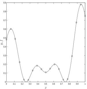
The detailed implementationand accuracy of the IRBFN method were reported previously (Mai-Duy and Tran-Cong, 2002). In all of numerical examples carried out in this paper, the value of is simply chosen to be in the range of 7 to 10. Before introducing the IRBFN interpolation into the BEM scheme, the performance of the IRBFN method and that of the element-based method are compared using the interpolation of the following function

y = 0:02(12 + 3s;3:5s 2

+ 7:2s3

)(1 + cos4s)(1 + 0:8sin3s)

(8)

where 0 s 1 (Figure 1). The accuracy achieved by each technique is evaluated via

the norm of relative error of the solution Ne dened by

Ne =

Pq

i=1(y(s (i))

;f(s (i)))2 Pq

i=1y(s (i))2

1=2

(12)

wherey(s(i)) andf(s(i)) are the exact and approximate solutions at the pointi respectively

and q is the number of test points. The performance of linear, quadratic and IRBFN

interpolations are assessed using four data sets of 13, 15, 17 and 19 known points. For each data set, the functiony is estimated at 500 test points. Note that the known and test points here are uniformly distributed. The results obtained using = 10 are displayed in Figure 2 showing that the IRBFN method achieves superior accuracy and convergence rate to the element-based method. The solution converges apparently asO(h1:95),O(h1:98)

and O(h9:47) for linear, quadratic and IRBFN interpolations respectively, where h is the

grid point spacing. At h = 0:06 which corresponds to a set of 19 grid points, the error norms obtained are 4:06e;2, 1:81e;2 and 1:98e;4 for linear, quadratic and IRBFN

schemes respectively.

(9)

3 A new interpolation method for the evaluation of

Boundary Integrals (BIs)

For heat transfer problems, the governing equations take the form

r

2u = b

x

2 (13)

u = u

x

2;u (14)

q

@u

@n = q

x

2;q (15)

whereu is the temperature, q is the temperature gradient across the surface,

n

is the unit outward normal vector, u and q are the prescribed boundary conditions, b is a known function of position and ;= ;u+ ;q is the boundary of the domain .

Integral Equation (IE) formulations for heat transfer problems are well documented in a number of texts Banerjee and Buttereld, 1981 Brebbia et al, 1984] where interested readers are referred for more details. Equations (13)-(15) can be reformulated in terms of integral equations for a given spatial point as follows

c()u() +Z

;

q(x)u(x)d; +

Z

b(x)u(x)d =

Z

;

u(x)q(x)d; (16)

where u is the fundamental solution to the Laplace equation, e.g. for a two dimensional

isotropic domain u = (1=2)ln(1=r) in which r is the distance from the point to the

current point of integration x, q =@u=@n, c() = =2 with being the internal angle

of the corner in radians if is a boundary point and c() = 1 if is an internal point. Note

(10)

that the volume integral here does not introduce any unknowns because the function b is given and furthermore it can be reduced to boundary integrals by using the Particular Solution (PS) techniques (Zheng et al, 1991) or the Dual Reciprocity Method (DRM) (Partridge et al, 1992). Without loss of generality, the following discussions are based on Equation (16) with b = 0 (Laplace's equation).

For the standard BEM, the numerical procedure for (16) involves a subdivision of the boundary ;into a number of small elements. On each element, the geometry and the variation of u and q are assumed to have a certain shape such as linear and quadratic ones. The study on interpolation of function in section 2 shows that the IRBFN inter-polation achieves an accuracy and convergence rate superior to the linear and quadratic element-based interpolations. The question here is whether the employment of IRBFN interpolation in the BEM scheme can improve the solution in terms of accuracy and convergence rate as in the case of function approximation. The answer is positive and substantiated in the remainder of this paper.

The rst issue to be considered is about the implementation of singular integrals when IRBFNs are present within integrands. The dierence between IRBFN interpolation and Lagrange-type interpolation is that in the present IRBFN interpolation, none of the basis functions are null at the singular point (the point where the eld point x and the source point coincide) and hence the corresponding integrands obtained are not regular. Consequently, at the singular point all CPV integrals associated with the IRBFN weights are singular and cannot be evaluated by using directly the hypothesis of constant potential over the whole domain as in the case of standard BEM. To overcome this diculty, the

(11)

treatment of singular CPV integrals needs to be slightly modied. The BIEs can be written in the following form (Tanaka et al, 1994 and Hwang et al, 2002)

u()

Z

;

"" !0

q(x)d; + CPV

Z

;

q(x)u(x)d; =

Z

;

u(x)q(x)d; (17)

where ;"is part of a circle that excludes its origin (or the singular point) from the domain

of analysis. Assume that the temperature u(x) is constant unit on the whole domain, i.e. u() = u(x) = 1, and hence the gradient q(x) is everywhere zero. Equation (17) then simplies to

Z

;""!0

q(x)d; =

;CPV Z

;

q(x)d;: (18)

Substitution of (18) into (17) yields

CPV Z

;

q(x)(u(x)

;u())d; =

Z

;

u(x)q(x)d;: (19)

The CPV integral is now written in the non-singular form where standard Gaussian quadrature can be applied. For weakly singular integrals, some well-known treatments such as logarithmic Gaussian quadrature and Telles' transformation technique (Telles, 1987) can be applied directly as in the case of standard BEM.

The second issue is concerned with the employment of the IRBFNs in the BEM scheme to represent the variables in boundary integrals. In the present method, the boundary ; of the domain of analysis is also divided into a number of segmentsNs, i.e. ; =PN

s

j=1;j

which are 1D domains to be represented by networks. Note that the size of segment ;j

(12)

can be much larger than the size of elements in the standard BEM provided that the associated boundary is smooth and the prescribed boundary conditions are of the same type. Equation (19) can be written in the discretised form as

Ns X j=1 Z ; j

q(x)(u

j(x);ul())d;j =

Ns X j=1 Z ; j

u(x)q

j(x)d;j (20)

where subscript j denotes general segments and the subscript l indicates the segment containing the source point . The variation of temperature u and gradient q on segment ;j is now represented by IRBF networks in terms of the curvilinear coordinate s as

(Equation (9))

uj =

mj+2 X

i=1

w(i)

ujH(i)

j (s) (21)

qj =

mj+2 X

i=1

w(i)

qjH(i)

j (s) (22)

wheres 2;j, mj +2 is the number of IRBFN weights,fw (i)

ujg

mj+2

i=1 and fw

(i)

qjg

mj+2

i=1 are the

sets of weights of networks for the temperatureu and temperature gradient q respectively. Similarly, the geometry can be interpolated from the nodal value by using IRBFNs as

x1j =

mj+2 X

i=1

w(i)

x1jH (i)

j (s) (23)

x2j =

mj+2 X

i=1

w(i)

x2jH (i)

j (s): (24)

(13)

Substitution of (21) and (22) into (20) yields Ns X j=1 Z ; j q (s) mj+2 X i=1

w(i)

ujH(i)

j (s);

ml+2 X

i=1

w(i)

ulH(i)

l ()

!

d;j

= Ns X

j=1 Z

;j

u(s)

mj+2 X

i=1

w(i)

qjH(i)

j (s)

!

d;j (25)

or, Ns X j=1 ( mj+2 X i=1

w(i)

uj Z ; j q

(s)H(i)

j (s)d;j

!

;

ml+2 X

i=1

w(i)

ul Z ; j q

(s)H(i)

l (s)d;j

! )

= Ns X

j=1

mj+2 X

i=1

w(i)

qj

Z

;

j

u(s)H

(i)

j (s)d;j

!

(26)

wheremj which is the number of training points on the segment j, can vary from segment to segment. Equation (26) is formulated in terms of the IRBFN weights of networks for u and q rather than the nodal values of u and q as in the case of standard BEM. Locating the source point at boundary training points results in the underdetermined system of algebraic equations with the unknown being the IRBFN weights. Thus, the system of equations obtained which can have many solutions, needs to be solved in the general least squares sense. The preferred solution is the one whose values are smallest in the least squares sense (i.e. the norm of components is minimum). This can be achieved by using Singular Value Decomposition technique (SVD). The procedural ow chart can be briey summarised as follows

1. Divide the boundary into a number of segments over each of which the boundary is smooth and the prescribed boundary conditions are of the same type

(14)

2. Apply the IRBFN for approximation of the prescribed physical boundary conditions in order to obtain IRBFN weights which are the boundary conditions in the weight space

3. Form the system matrices associated with IRBFN weightswu and wq

4. Impose the boundary conditions obtained from the step 2 and then solve the system for IRBFN weights by SVD technique

5. Compute the boundary solution by using the IRBFN interpolation

6. Evaluate the temperature and its derivatives at selected internal points

7. Output the results.

Note that for the numerical solution of Poisson's equations using the BEM-PS approach, the particular solution is rst found by expressing the known functionb as a linear combi-nation of radial basis functions and the volume integral is then transformed into boundary integrals (Zheng et al, 1991). However, the rst stage of this process produces a certain error which is separate from the error in the evaluation of boundary integrals. In order to conne the error of solution only to the evaluation of BIs, the following numerical exam-ples of heat transfer problems governed by Laplace's equations or by Poisson's equations are chosen where the associated analytical particular solutions exist for the latter.

(15)

4 Numerical examples

In this section, the proposed method is veried and compared with the standard BEM on heat transfer problems governed by Laplace's or Poisson's equations. In order to make the BEM programs general in the sense that they can deal with any types of boundary conditions at the corners, all BEM codes here with linear, quadratic and IRBFN interpolations employ discontinuous elements at the corner. The extreme boundary point at the corner is shifted into the element by a 1=4 of the length of the element. Integrals are evaluated by using standard Gaussian quadrature for regular cases and logarithmic Gaussian quadrature or Telles' quadratic transformation (Telles, 1987) for weakly singular cases with 9 integration points. For the purpose of error estimation and convergence study, the error norm dened in (12) will be utilised here with the function y being the temperature u and its normal derivative q in the case of the boundary solution, or the temperatureu in the case of the internal solution.

4.1 Boundary geometry with straight lines

It can be seen that the linear interpolation is able to represent exactly the geometry for a straight line and hence on the straight line segment the IRBFN interpolation needs only to be used for representing the variation of temperature and gradient.

(16)

4.1.1 Example 1

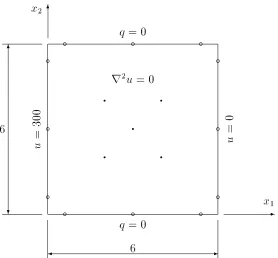
Consider a square closed domain whose dimensions are taken to be 6 units by 6 units as depicted in Figure 3. The temperature on the left and right edges is maintained at 300 and 0 respectively while the homogeneous Neumann conditions q = 0 are imposed on the other edges. Inside the square the steady state temperature satises Laplace's equation. The analytical solution is

u(x1x2) = 300 ;50x

1:

This is a simple problem where the variation of temperature is linear. It can be seen that the use of linear interpolation is the best choice for this problem. Both linear and IRBFN ( = 10) interpolations are employedand the corresponding BEM results on the boundary and at some internal points are displayed in Table 1 showing the proposed method works as well as the linear-BEM. Signicantly, the IRBFN-BEM works increasingly better than the linear-BEM as the number of boundary points increases which seems to indicate that the IRBFN-BEM does not suer numerical ill-conditioning as in the case of the standard BEM. Note that in the case of the IRBFN interpolation, each edge of the square domain and the boundary points on it become the domain and training points of the network associated with the edge respectively. It is expected that the IRBFN-BEM approach performs better in dealing with higher order variations of temperature, which is veried in the following examples.

(17)

4.1.2 Example 2

The problem is to nd the temperature eld such that

r

2u = 0 inside the square 0

x 1

0 x 2

(27)

u(x1) = sin(x1) on the top edge (0 x

1

) (28)

u(x1x2) = 0 on the other three sides. (29)

The exact solution of this problem is given by (Snider, 1999)

u(x1x2) = 1

sinh() sin(x1)sinh(x2):

This is a Dirichletproblem for which the essential boundary condition is imposed along the boundary. Using discontinuous boundary elements at the corner for the case of standard BEM or shifting the training points at the corner into adjacent segments for the case of IRBFN-BEM allow the correct description of multi-valued gradient q at the corner. In the case of IRBFN interpolation, each side of the square domain becomes the domain of network and the boundary points on it are utilised as training points. To study the convergence of the present method, four boundary point densities, namely 54, 74,

94 and 114, and = 7 are employed. Some internal points are selected at (=3=3),

(=32=3), (=2=2), (2=3=3) and (2=32=3). The performance of the BEM with linear, quadratic and IRBFN interpolations is assessed using error norms of the boundary solution and the internal solution. The boundary solution is displayed in Figure 4 showing that the proposed method is the most accurate one with higher convergence rate achieved.

(18)

With these given boundary point densities, the solution converges asO(h2:24),O(h2:04) and

O(h3:83) for linear, quadratic and IRBFN interpolations respectively. Ath = 0:31 which

corresponds to the boundary point density of 114, error norms obtained are 1:27e;2,

1:17e;2 and 2:80e;5 for linear, quadratic and IRBFN interpolations respectively. The

internal results are recorded in Table 2 showing the IRBFN-BEM achieves a solution accuracy better than the linear/quadratic-BEM results by several orders of magnitude.

4.1.3 Example 3

The problem is to nd the temperature eld such that

r

2u = 0 inside the square 0

x 1

0 x 2

(30)

u(x2) = sin

3

(x2) on the right edge (0 x

2

) (31)

u(x1x2) = 0 on the other three sides. (32)

The analytical solution of this problem (Snider, 1999) is

u(x1x2) =

3

4sinh() sin(x2)sinh(x1) ;

1

4sinh(3) sin(3x2)sinh(3x1):

The shape of this solution is more complicated than the one in the previous example and provides a good test for the present method. The boundary point densities are chosen to be 94, 114, 134 and 154. The selected internal points are (=3=3), (=32=3),

(=2=2), (2=3=3) and (2=32=3). The proposed method here also performs much better than the standard BEM and similar remarks as mentioned in Example 2 apply.

(19)

With = 7, error norms of the boundary solution and the internal solution are displayed in Figure 5 and Table 3 respectively. The rates of convergence of the boundary solution are of O(h2:14), O(h1:38) and O(h4:78) for linear, quadratic and IRBFN interpolations

respectively. Ath = 0:07 which corresponds to the boundary point density of 154, the

achieved error norms are 3:91e;2, 2:79e;2 and 6:88e;5 for linear, quadratic and IRBFN

interpolations respectively. The accuracy of the internal solution by the present method is also better, by several orders of magnitude, than the ones by linear and quadratic BEMs. Furthermore, the CPU time requirements for the two methods are compared in Table 4. The structures of the MATLAB codes are the same and therefore it is believed that the higher eciency achieved by the IRBFN-BEM is due to the fact that the number of segments (elements) used in the IRBFN-BEM is signicantly less than that used in the standard BEM, resulting in a better vectorised computation for the former (MATLAB's internal vectorisation).

4.2 Boundary geometry with curved and straight segments

Neural networks are employed here to interpolate not only the variables u and q by using (21) and (22) but also the geometry of curved segments by using (23) and (24). All

quantities in the boundary integrals such as u, q and d;are represented by IRBFNs

necessarily in terms of the curvilinear coordinate (arclength) s. Special attention here is given to the transformation of the quantityd;from rectangular to curvilinear coordinates

(20)

where the use of a Jacobian is required as follows d; = @x1 @s 2 + @x2 @s 2 !

1=2

ds (33)

in which the derivatives ofx1 and x2 on the segment ;j can be expressed in terms of basis

function H (6) as

@x1j

@s =

mj+2 X

i=1

w(i)

x1jH (i)

j (s) (34)

@x2j

@s =

mj+2 X

i=1

w(i)

x2jH (i)

j (s): (35)

Clearly, these derivatives can be calculated straightforwardly once the interpolation of the function is done after solving (23)-(24). For more details covering the calculation of derivative functions by IRBFNs, the reader is referred to Mai-Duy and Tran-Cong (2002). Normally, the orders of IRBFN approximation for the boundary geometry and the variation of u and q are chosen to be the same. However, they can be dierent and are discussed shortly.

4.2.1 Example 4

Consider the boundary value problem governed by Laplace equation

r 2

u = 0

(21)

as depicted in Figure 6. The domain of analysis is one quarter of the ellipse and the boundary conditions are

u = 0

on OA and BO and

@u

@n =;

a2 ;b

2

(a4x 2

2+b 4x

2

1) 1=2x

1x2

on AB witha and b being the half lengths of the major and minor axes respectively. This

problem with a = 10 and b = 5 was solved by quadratic BEM (Brebbia and Dominguez,

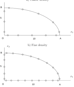
1992) using 5 and 10 quadratic elements with two selected internal points being (2, 2) and (4, 3.5). For the present method, the boundary is divided into 3 segments (two straight lines and one curve) and the training points are taken to be the same as the boundary nodes used in the case of quadratic BEM. Thus the densities are 5, 5 and 3 on segments OA, AB and BO respectively which corresponds to the case of 5 quadratic elements and densities 9, 9 and 5 corresponding to the case of 10 quadratic elements. In order to compare the present results with the results by quadratic BEM (Brebbia and Dominguez, 1992) and the exact solution, some values of function u are extracted and the errors obtained by the two methods are displayed in Tables 5 and 6 which show that the present method yields better accuracy. For example, with 4 digit scaled xed point, for the coarse density the range of the error is (0.02%-0.2%) and (0.84%-2.32%) for IRBFN-BEM and quadratic BEM respectively while for the ne density the error range is (0.00%-0.02%) and (0.02%-0.14%) for IRBFN-BEM and quadratic BEM respectively.

(22)

4.2.2 Example 5

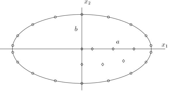
The distribution of functionu in an ellipse with a semi-major axis a = 2 and a semi-minor axis b = 1 is described by

r 2u =

;2 (36)

subject to the condition u = 0 along the boundary ;. The exact solution is

u(x1x2) = ;0:8

x2 1

a2 + x 2

2

b2 ;1

:

This problem is governed by Poisson's equation and hence the BEM with PS can be applied here for obtaining numerical solution. The solution u can be decomposed into a homogeneous part uH _{and a particular solution part} _uP _as

u = uH ₊_uP_:

The particular solution to equation (36) can be veried to be

uP ₌

;

x2 1+x

2

while the complementary one satises the Laplace's equation r

2uH = 0 with boundary

condition uH ₌;uP on ;. The latter is to be solved by BEM. Partridge et al (1992) used

this approach to solve the problem in which 16 linear boundary elements are employed and the solution obtained was displayed at 7 internal points. In the present method,

(23)

the boundary ;is divided into 2 segments as shown in Figure 7. Four data densities,

namely 92, 112, 132 and 152, and = 8 are employed here to simulate the

problem. Error norms of the boundary solution obtained are 0.0105, 0.0037, 9:4436e;4

and 5:8135e;4 for the four densities respectively with the convergence rate achieved being

O(N(;5:9289)), whereN is the number of training boundary points employed (Figure 8). In

order to compare with the linear BEM (Partridge, 1992), the solution at 7 internal points is also computed by the present method and the corresponding error norms obtained are 0.0063, 0.0026, 8:0387e;4 and 3:4900e;5 for the four densities respectively. Hence with

the coarse density of 92 that corresponds to 16 linear boundary elements, the present

method achieves the error norm of 0.0063, while linear BEM achieves only Ne = 0:0109. The latter number is calculated by the present authors using the table shown in Partridge et al (1992). Numerical result for the nest density is displayed in Table 7.

4.2.3 Interpolation for geometry and boundary variables

In the last two examples, the IRBFN interpolations for the geometry and the variables u and q have the same order, i.e. the training points used are the same for both cases. However, the order of IRBFN interpolation can be chosen dierently for the geometry and the variables u and q in order to be able to obtain high quality solutions with as low as possible a cost. The geometry is usually known and hence the number of training points for the geometry interpolation can be estimated. It is emphasised that the size of the nal system of equations only depends on the order of IRBFN interpolation for the variables u and q and hence in the case of highly curved boundary, it is recommended that the order

(24)

of IRBFN interpolation can be chosen higher for the geometry than for the variables u andq. The problem in the last example is solved again with increasing number of training points for the geometry interpolation. The density of training points employed is 92

for the variables u and q while they are 122 and 142 for the geometry. The solution

is improved as shown in Table 8. For example, the error norm of the boundary solution decreases from 0.0105 for the normal case (the same order) to 9:5093e;4 and 8:2902e;4

for increasing order of geometry interpolation.

5 Concluding remarks

In this paper, the introduction of Indirect RBFN interpolation into the BEM scheme to represent the variables in BIEs for numerical solution of heat transfer problems is imple-mented and veried successfully. Numerical examples show that the proposed method considerably improves the estimate of the boundary integrals resulting in better solutions not only in terms of the accuracy but also in terms of the rate of convergence. The CPV integral is written in the non-singular form where standard Gaussian quadrature can be applied while the weakly singular integrals are evaluated by using the well-known numer-ical techniques as in the case of standard BEM. The method can be extended to problems of viscous ows which will be carried out in future work.

Acknowledgement

This work is supported by a Special USQ Research Grant (Grant No 179-310) to Thanh Tran-Cong. This support is gratefully acknowledged. The authors would like to thank the referees for their helpful comments.

(25)

References

Banerjee, P.K. and Buttereld, R. 1981. Boundary Element Methods in Engineering

Science. McGraw-Hill, London

Brebbia, C.A. and Dominguez, J. 1992. Boundary Elements: An Introductory Course.

Computational Mechanics Publications, Southampton

Brebbia, C.A., Telles, J.C.F. and Wrobel, L.C. 1984. Boundary Element Techniques:

Theory and Applications in Engineering. Springer-Verlag, Berlin

Cybenko, G. 1989. Approximation by superpositions of sigmoidal functions. Mathemat-ics of Control Signals and Systems,

2

, 303-314

Girosi, F. and Poggio, T. 1990. Networks and the best approximation property. Biolog-ical Cybernetics,

63

, 169-176

Haykin, S. 1999. Neural Networks: A Comprehensive Foundation. Prentice-Hall, New

Jersey

Hwang, W.S., Hung, L.P. and Ko, C.H. 2002. Non-singular boundary integral formu-lations for plane interior potential problems. International Journal for Numerical Methods in Engineering,

53

(7), 1751-1762

Kansa, E.J. 1990. Multiquadrics- A scattered data approximation scheme with appli-cations to computational uid-dynamics-II. Solutions to parabolic, hyperbolic and elliptic partial dierential equations. Computers and Mathematics with Applica-tions,

19

(8/9), 147-161

(26)

Mai-Duy, N. and Tran-Cong, T. 2001a. Numericalsolution of dierential equations using multiquadric radial basis function networks. Neural Networks,

14

(2), 185-199 Mai-Duy, N. and Tran-Cong, T. 2001b. Numerical solution of Navier-Stokes equations

using multiquadric radial basis function networks. International Journal for Nu-merical Methods in Fluids,

37

, 65-86

Mai-Duy, N. and Tran-Cong, T. 2002. Mesh-free radial basis function network methods with domain decomposition for approximation of functions and numericalsolution of Poisson's equations. Engineering Analysis with Boundary Elements,

26

(2), 133-156 Partridge, P.W., Brebbia, C.A. and Wrobel, L.C. 1992. The Dual Reciprocity Boundary

Element Method. Computational Mechanics Publications, Southampton

Press, W.H., Flannery, B.P., Teukolsky, S.A. and Vetterling, W.T. 1988. Numerical

Recipes in C: The Art of Scientic Computing. Cambridge University Press, Cam-bridge

Sharan, M., Kansa, E.J. and Gupta, S. 1997. Application of the multiquadric method for numerical solution of elliptic partial dierential equations. Journal of Applied Science and Computation,

84

, 275-302

Sladek, V. and Sladek, J. 1998. Singular Integrals in Boundary Element Methods. Com-putational Mechanics Publications, Southampton

Snider, A. D. 1999. Partial Dierential Equations: Sources and Solutions. Prentice-Hall, Upper Saddle River, NJ 07458

(27)

Tanaka, M., Sladek, V. and Sladek, J. 1994. Regularization techniques applied to bound-ary element methods. Applied Mechanics Reviews,

47

, 457-499

Telles, J.C.F. 1987. A self-adaptive co-ordinate transformation for ecient numerical evaluation of general boundary element integrals. International Journal for Numer-ical Methods in Engineering,

24

, 959-973

Zerroukat, M., Power, H. and Chen, C.S. 1998. A numerical method for heat transfer problems using collocation and radial basis functions. International Journal for Numerical Methods in Engineering,

42

, 1263-1278

Zheng, R., Coleman, C.J. and Phan-Thien, N. 1991. A boundary element approach for non-homogeneous potential problems. Computational Mechanics,

7

, 279-288

(28)

Table 1: Example 1 - Error norms Nes of IRBFN-BEM and linear-BEM solutions. The

selected internal points are (2,2), (2,4), (3,3), (4,2) and (4,4). In the rst row,nm means

n boundary points per segment and m segments. The number of boundary elements in each case results in the same total number of boundary points.

Boundary points 34 44 54 64

Linear elements 8 12 16 20

Error norm of the boundary solution

Linear-BEM 3.01e-7 3.08e-7 3.72e-7 4.30e-7

IRBFN-BEM 7.22e-6 1.17e-6 4.33e-7 1.60e-7 Error norm of the internal solution

Linear-BEM 1.86e-7 1.43e-7 1.22e-7 1.07e-7

IRBFN-BEM 3.97e-6 4.07e-7 1.57e-7 5.17e-8

(29)

Table 2: Example 2 - Error norms Nes of the internal solution obtained by BEM with

dierent interpolation techniques. The IRBFN-BEM yields a solution more accurate than the linear/quadratic-BEM one by several orders of magnitude.

Linear 2.96e-2 1.25e-2 6.90e-3 4.30e-3

Quadratic 2.80e-3 5.90e-4 1.82e-4 7.66e-5

IRBFN 1.27e-5 4.79e-7 1.49e-7 3.40e-8

(30)

Table 3: Example 3 - Error norms Nes of the internal solution obtained by BEM with

dierent interpolation techniques. The IRBFN-BEM yields a solution more accurate than the linear/quadratic-BEM one by several orders of magnitude.

Linear 6.60e-3 4.20e-3 2.90e-3 2.20e-3

Quadratic 3.25e-4 1.74e-4 7.84e-5 4.09e-5

IRBFN 2.79e-6 1.91e-6 7.97e-7 9.64e-7

(31)

Table 4: Example 3: CPU times (s) used to obtain the boundary solution and the total solution by Linear-BEM and IRBFN-BEM. The code is written in the MATLAB language (version R11.1 by The MathWorks, Inc.), which is run on a 548-MHz Pentium PC. Note that MATLAB language is interpretative.

Mesh Linear-BEM IRBFN-BEM

boundary solution total solution boundary solution total solution

99 1:98 4.57 2:07 2.19

1111 3:02 8.39 3:08 3.27

1313 4:29 13.88 4:27 4.63

1515 5:78 21.56 5:70 6.33

(32)

Table 5: Example 4 - Comparison of the error obtained by the present IRBFN-BEM ( = 7) and the quadratic BEM using the same boundary nodes (5 quadratic elements).

x1 x2 u u Error(%) u Error(%)

Exact IRBFN-BEM Quadratic BEM

8.814 2.362 -12.489 -12.514 0.20 -12.779 2.32

6.174 3.933 -14.570 -14.579 0.06 -14.839 1.85

3.304 4.719 -9.356 -9.354 0.02 -9.435 0.84

2.000 2.000 -2.400 -2.404 0.17 -2.431 1.29

4.000 3.500 -8.400 -8.413 0.15 -8.472 0.86

(33)

Table 6: Example 4 - Comparison of the error obtained by the present IRBFN-BEM ( = 7) and the quadratic BEM using the same boundary nodes (10 quadratic elements).

x1 x2 u u Error(%) u Error(%)

Exact IRBFN-BEM Quadratic BEM

8.814 2.362 -12.489 -12.487 0.02 -12.506 0.14

6.174 3.933 -14.570 -14.568 0.01 -14.576 0.04

3.304 4.719 -9.356 -9.355 0.01 -9.363 0.07

2.000 2.000 -2.400 -2.400 0.00 -2.399 0.04

4.000 3.500 -8.400 -8.400 0.00 -8.402 0.02

(34)

Table 7: Example 5 - The boundary solution obtained by the present IRBFN-BEM using

the density of 152. Although no symmetry condition was imposed in the numerical

model, the results obtained are accurately symmetrical. Owing to symmetry,the displayed results corresponds to only a quarter of the elliptical domain.

Coordinates Exact Computed

x1 x2 Gradient q Gradient q

1.997 0.056 -0.804 -0.802

1.950 0.223 -0.857 -0.859

1.802 0.434 -1.001 -1.000

1.564 0.623 -1.177 -1.178

1.247 0.782 -1.347 -1.347

0.868 0.901 -1.483 -1.483

0.445 0.975 -1.570 -1.570

0.000 1.000 -1.600 -1.600

(35)

Table 8: Example 5 - Error norms obtained by the present method with increasing order of the IRBFN interpolation for the geometry. The densities of IRBFN interpolation are 92 for the boundary variables and 92, 122 and 142 for the geometry.

Ne 92 122 142

boundary solution 0.0105 9:5093e;4 8:2902e;4

internal solution 0.0063 1:5961e;4 9:8966e;5

(36)

0 0.1 0.2 0.3 0.4 0.5 0.6 0.7 0.8 0.9 1 0

0.1 0.2 0.3 0.4 0.5 0.6 0.7 0.8 0.9

x

y

f

Figure 1: Interpolation of function y = 0:02(12 + 3x;3:5x

2+ 7:2x3)(1 + cos4x)(1 +

0:8sin3x) from a set of grid points. Legends |: exact function,: grid point.

[image:36.612.152.453.39.348.2]

(37)

10−1 10−4

10−3 10−2 10−1

Grid Point Spacing

Ne

Figure 2: Interpolation of function y = 0:02(12 + 3x;3:5x

2+ 7:2x3)(1 + cos4x)(1 +

0:8sin3x): The rate of convergence with grid point spacing renement. Legends: linear, 2: quadratic and4: IRBFN. The solution converges apparently as O(h

1:95),O(h1:98) and

O(h9:47) for linear, quadratic and IRBFN interpolations respectively, where h is the grid

point spacing.

[image:37.612.151.451.42.350.2]

(38)

u=3

00

u=0

q = 0 q = 0

6

x2

-x1

6

?

6 6

r 2u = 0

Figure 3: Example 1 - Geometry, boundary conditions, boundary points and internal points.

[image:38.612.114.392.213.471.2]

(39)

100 10−5

10−4 10−3 10−2 10−1 100

h

Ne

Figure 4: Example 2 - Error norm Ne of the boundary solution versus boundary point

spacing h obtained by BEM with dierent interpolation techniques. Legends 4: linear,

2: quadratic and : IRBFN. With the given boundary point densities of 54, 74,

94 and 114, the rate of convergence appears to be O(h

2:24),O(h2:04) andO(h3:83) for

linear, quadratic and IRBFN interpolations respectively as depicted by solid lines. The proposed method achieves accuracy and convergence rate superior to the element-based method.

[image:39.612.149.453.37.285.2]

(40)

10−1 100 10−5

10−4 10−3 10−2 10−1 100

h

Ne

Figure 5: Example 3 - Error norm Ne of the boundary solution versus boundary point

spacingh obtained from BEM with dierent interpolation techniques. Legends 4: linear, 2: quadratic and : IRBFN. With the given boundary point densities of 94, 114,

134 and 154, the rate of convergence appears to beO(h

2:14),O(h1:38) andO(h4:78) for

linear, quadratic and IRBFN interpolations respectively as depicted by solid lines. The proposed method achieves accuracy and convergence rate superior to the element-based method.

[image:40.612.149.453.38.284.2]

(41)

O A B

10 5

O _A

B

10 5

x1

x2

x1

x2

a) Coarse density