Theses Thesis/Dissertation Collections
7-2018
Exploring High Level Synthesis to Improve the
Design of Turbo Code Error Correction in a
Software Defined Radio Context
Bradley E. Conn
Follow this and additional works at:https://scholarworks.rit.edu/theses
This Thesis is brought to you for free and open access by the Thesis/Dissertation Collections at RIT Scholar Works. It has been accepted for inclusion in Theses by an authorized administrator of RIT Scholar Works. For more information, please [email protected].
Recommended Citation
Software Defined Radio Context
Software Defined Radio Context
Bradley E. Conn
July 2018
A Thesis Submitted in Partial Fulfillment of the Requirements for the Degree of
Master of Science in
Computer Engineering
Software Defined Radio Context
Bradley E. Conn
Committee Approval:
Dr. Sonia Lopez Alarcon Advisor Date
RIT, Department of Computer Engineering
Dr. Marcin Lukowiak Date
RIT, Department of Computer Engineering
Dr. Andres Kwasinski Date
With the ever improving progress of technology, Software Defined Radio (SDR) has
become a more widely available technique for implementing radio communication.
SDRs are sought after for their advantages over traditional radio communication
mostly in flexibility, and hardware simplification. The greatest challenges SDRs face
are often with their real time performance requirements. Forward error correction
is an example of an SDR block that can exemplify these challenges as the error
correction can be very computationally intensive. Due to these constraints, SDR
im-plementations are commonly found in or alongside Field Programmable Gate Arrays
(FPGAs) to enable performance that general purpose processors alone cannot achieve.
The main challenge with FPGAs however, is in Register Transfer Level (RTL)
de-velopment. High Level Synthesis (HLS) tools are a method of creating hardware
descriptions from high level code, in an effort to ease this development process. In
this work a turbo code decoder, a form of computationally intensive error correction
codes, was accelerated with the help of FPGAs, using HLS tools. This accelerator was
implemented on a Xilinx Zynq platform, which integrates a hard core ARM processor
alongside programmable logic on a single chip.
Important aspects of the design process using HLS were identified and explained.
The design process emphasizes the idea that for the best results the high level code
should be created with a hardware mindset, and written in an attempt to describe a
hardware design. The power of the HLS tools was demonstrated in its flexibility by
providing a method of tailoring the hardware parameters through simply changing
values in a macro file, and by exploration the design space through different data
types and three different designs, each one improving from what was learned in the
previous implementation. Ultimately, the best hardware implementation was over
56 times faster than the optimized software implementation. Comparing the HLS
Signature Sheet i
Dedication ii
Abstract iii
Table of Contents v
List of Figures viii
List of Tables 1
1 Introduction 2
1.1 Introduction . . . 2
1.1.1 Software Defined Radio . . . 2
1.1.2 Turbo Codes . . . 3
1.1.3 Field Programmable Gate Arrays . . . 4
1.1.4 High Level Synthesis . . . 4
1.2 Related Works . . . 5
2 Software Defined Radio 8 2.1 Software Defined Radio . . . 8
2.1.1 Common Radio Principals . . . 9
2.1.2 Ideal SDR . . . 10
2.1.3 Open Source SDR C and C++ Libraries . . . 11
3 Turbo Codes 13 3.1 Turbo Code Error Correction . . . 13
3.1.1 Turbo Code Encoder . . . 14
3.1.2 Turbo Code Decoder . . . 15
3.1.3 Implementations . . . 23
4 High Level Synthesis Guidelines 26 4.1 Understand The Tool Offerings . . . 27
4.1.1 IDE Features . . . 27
4.1.3 Data Types and Libraries . . . 29
4.2 Coding Style . . . 30
4.2.1 Bounded Loop Iterators . . . 31
4.2.2 Being Explicit Where Possible . . . 32
4.2.3 Single Return Point . . . 35
4.3 Write Code That Emulates Hardware . . . 36
5 HLS MAX-MAP Implementation 39 5.1 High Level Designs . . . 39
5.1.1 Software . . . 40
5.1.2 Hardware Design 1: Initial Sliding Window . . . 41
5.1.3 Hardware Design 2: Replicated Hardware . . . 46
5.1.4 Hardware Design 3: Fully Pipelined . . . 50
5.2 Design Trade-off Analysis . . . 53
5.3 Low level implementations . . . 56
5.3.1 Calculation Units . . . 57
5.3.2 Circular Buffer . . . 58
5.3.3 Dependencies . . . 58
5.3.4 Data Types . . . 59
5.4 Flexibility . . . 62
5.5 Accelerator Integration . . . 63
5.5.1 Accelerator Interface . . . 63
5.5.2 Issues Running On The Board . . . 67
6 Results 69 6.1 Zynq Platform . . . 69
6.2 Designs used for testing . . . 70
6.2.1 Parameters . . . 71
6.3 Hardware vs Software . . . 72
6.3.1 Software Designs . . . 72
6.3.2 Hardware vs Software . . . 73
6.3.3 Hardware Resource Utilizations . . . 77
6.4 HLS vs Manually Optimized Design . . . 79
7 Conclusion and Future Work 83 7.1 Conclusions . . . 83
7.3 Future Work . . . 85
Bibliography 86
8 Appendix 89
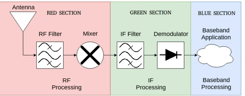
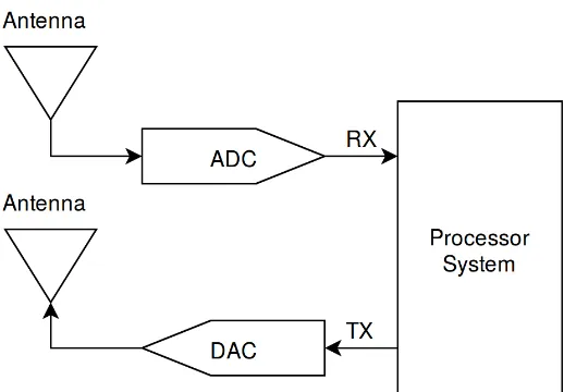
2.1 An example superheterodyning receiver to display the partitioning of the RF, IF, and baseband signals. An SDR can sample at any of the points along the path. . . 10 2.2 The ideal SDR receiver and transmitter made up of an antenna,
AD-C/DAC and processing system. . . 11
3.1 A simplified example of how turbo codes are integrated into radio com-munication. . . 13 3.2 An example of a memory 2 Recursive Systematic Convolutional (RSC)
Encoder. . . 14 3.3 An example of a turbo code encoder containing two RSC encoders. . 14 3.4 A high level view of the turbo code decoder consisting of MAP
de-coders, interleavers, deinterleavers, and a hard decision maker. The bold lines highlight the feedback loop present in the turbo decoder. . 15 3.5 The state machine representing the example RSC encoder. The
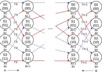
en-coder memory is shown in the parenthesis. Inputs of zero are shown as dotted lines, and inputs of one are shown with full lines. The input and output format is represented as input/output marked on the transition lines. . . 16 3.6 This diagram represents a trellis with 5 states over 4 bits. The red
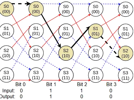
lines represent an input bit of one and the dotted blue lines represent and input bit of zero. . . 16 3.7 This diagram shows an example of how an encoded sequence can be
represented with the trellis. The bolded black lines represent a path that the sequence could take. . . 17 3.8 This diagram shows how the Gamma, Alpha, and Beta terms are
rep-resented in the trellis. The Gamma terms are the state transitions represented by the Γn in the diagram. The Alpha terms are denoted
byAn and move left to right. The Beta terms are denoted by BN and
move right to left. . . 20 3.9 Bit Error Rate performance of a MAX-MAP turbo code decoder with
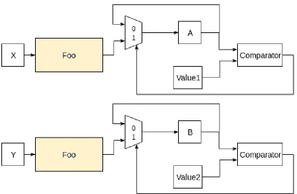
4.1 Illustration of the hardware interpretation when mutual exclusion is not proven. In this case two separate foo units are required. . . 33 4.2 Illustration of the hardware interpretation when mutual exclusion is
proven. In this case one foo unit can be shared. . . 34 4.3 Example of resulting hardware from listing 4.7 . . . 37 4.4 Example of resulting hardware from listing 4.8 . . . 38
5.1 The high level flow of data for the original MAP decoder. The N inputs represents the entire block of information received. Each of the terms are calculated separately in their entirety before continuing to the next calculations. . . 40 5.2 The sliding window approach shown on a trellis structure. In this
example a window of 5 and a hop of 2 is used. . . 42 5.3 The high level hardware design for the initial sliding window approach.
N represents the number of inputs in the block, W represents the num-ber of inputs in the window, and H represents the amount to hop by for each window. Each of the inner loops is pipelined in this design. . 43 5.4 The second high level hardware design. This is the same as the
pre-vious design except with multiple parallel Beta Calculation Units. In this diagram nB represents the number of parallel Beta Calculation Units, N represents the number of inputs in the block, W represents the number of inputs in the window, and H represents the amount to hop by for each window. Again each of the inner loops is pipelined in this design. . . 47 5.5 The third high level hardware design. This design also has parallel Beta
Calculation Units but is different in that the entire design is pipelined instead of just the inner loops so each of the calculation units have the ability to run in parallel. In this diagram nB represents the number of parallel Beta Calculation Units, N represents the number of inputs in the block, W represents the number of inputs in the window, and H represents the amount to hop by for each window. . . 50 5.6 The fixed point BER performance compared to the floating point BER
performance. . . 61 5.7 The MAX MAP decoder integration using the Axi interface on the
5.8 The MAX MAP decoder integration using the BRAM interface on the Zynq board. . . 68
6.1 Simplified diagram of how the turbo code decoder and MAX-MAP Decoder accelerator is connected on the Zynq hardware. . . 70 6.2 Performance of the memory 3 hardware accelerator implementations
over the best software implementation. Block Size: 3200 Bits, Trellis Size: 8 States, Window Size: 32 Bits, Window Hop : 8 Bits, Beta Calculation Units: 4 Units . . . 75 6.3 Performance of the memory 4 hardware accelerator implementations
over the best software implementation. Block Size: 3200 Bits, Trellis Size: 16 States, Window Size: 32 Bits, Window Hop : 8 Bits, Beta Calculation Units: 4 Units . . . 75 6.4 The values that change in a single line to create unique
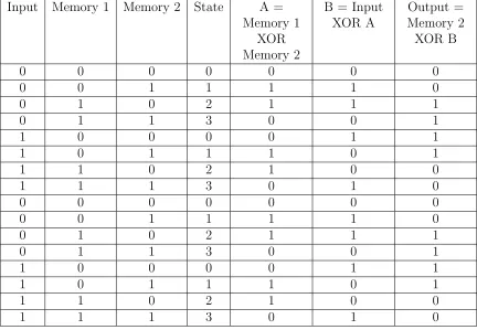
3.1 Truth table representation of the RSC encoder shown previously. . . . 19
6.1 ZCU102 Processor Specifications . . . 70
6.2 ZCU102 Programmable Logic Specifications . . . 70
6.3 Modifiable Implementation Parameters . . . 72
6.4 Value of Parameters which Remained Constant . . . 72
6.5 Memory 3 encoder software results . . . 73
6.6 Memory 4 encoder software results . . . 73
6.7 Optimized Software Results . . . 74
6.8 Memory 3 Hardware Results . . . 74
6.9 Memory 4 Hardware Results . . . 74
6.10 Memory 3 Resource Usage Table . . . 78
6.11 Memory 4 Resource Usage Table . . . 78
6.12 Throughput Table . . . 81
6.13 Memory 2 Hardware Results . . . 81
Introduction
1.1
Introduction
1.1.1 Software Defined Radio
The ever increasing power of digital technology as well as newly developed tools
have allowed software defined radio (SDR) to grow from an idea to a reality. SDRs
provide many advantages over traditional hardware radios including, flexibility,
cus-tomizability, longevity, reliability, and repurposability to name a few. SDR is a way
of implementing typical radio communication hardware, such as mixers, filters, gain
controllers, modulators, demodulators, using software.
The flexibility of SDR might be the most compelling aspect of the concept. SDRs
often allow a wide range of frequencies ranging from KHz to GHz to be used in a
single radio, which is uncommon for hardware radios. More importantly, SDRs can
potentially implement any protocol, or a range of protocols at once. In a common cell
phone for example, one might find different hardware specifically for Bluetooth, Wifi,
GPS, and GSM or CDMA communication. With SDR, all of these could potentially
be implemented in one, eliminating the need for separate dedicated hardware for the
different protocols.
The upgradability, reconfigurability, and repurposability are also enticing aspects
bugs, or change to suit entirely new applications. Additionally, this can also occur
remotely, which can have numerous benefits.
Reliability is another significant aspect of SDRs. Increased reliability can occur as
there is limited component tuning required, there are fewer components that can fail,
such as diodes or capacitors, and parameter differences, such as temperature change
or manufacturing variations, are limited.
Cost saving is another element that can be considered for SDRs. Cost savings
can occur as software can easily be reused for free, cutting down on design time
and material cost. This eliminates the need for expensive new hardware designs,
enabling low cost research development and testing. Additionally to this, little to no
maintenance is required.
Although SDRs have numerous advantages they also has very challenging
disad-vantages. The biggest one is that SDRs require a lot of processing power, increasing
power consumption, and potentially increasing cost. The technology behind it, such
as processors, Analog to Digitl Conveters (ADCs), and Digital to Analog Converters
(DACs), are not always fast enough for SDR applications. Additionally, the software
code can quickly become very complex.
1.1.2 Turbo Codes
One interesting SDR component is the error correction code block. Specifically, turbo
code error correction. Turbo codes are a widely used form of forward error
correc-tion that provides near channel capacity performance[1]. Their uses can be seen
from low signal to noise deep space satellites to real time cell phone communication.
For instance, the Long Term Evolution (LTE) standard uses turbo codes for error
correction[2] which requires low latency, and high reliability. Most implementations
of turbo codes can be found in integrated circuits due to their real time constraints
requirements however they pose a significant challenge for SDRs, but remain an
im-portant aspect for radio communication.
1.1.3 Field Programmable Gate Arrays
Even though software defined radios are accessible like never before, many
applica-tions are not able to run on truly general purpose processors alone. SDRs often require
accelerators in the forms of Digital Signal Processors (DSPs) or Field Programmable
Gate Arrays (FPGAs). FPGAs allow custom digital hardware functionality to be
implemented, and can be reconfigured to implement new functionality when desired.
They are particularly interesting for software defined radios due to their ability to
ac-celerate specific tasks. Turbo codes provide a great module for FPGA acceleration for
their complexity, computational requirements, and frequent use described previously.
Using an FPGA can have the advantage that the implementation can be tailored to
the application requirements, handling different parameters such as latency, resource
usage, power consumption, and accuracy.
1.1.4 High Level Synthesis
Even with the tremendous performance improvements FPGAs can provide, the most
daunting aspect is developing for them. Development can be long and difficult. An
ever evolving method for developing for FPGAs is through the use of High Level
Syn-thesis (HLS) tools. HLS provides a design flow in which algorithms are implemented
using high level languages such as C or C++. These implementations get interpreted
by the HLS tools, which generate Register Transfer Level (RTL) models of the
algo-rithm in a hardware description language such as VHDL or Verilog. This removes the
developer from many of the low level nuances required by manually optimized designs,
which comes at the cost of complete customization. Manually optimized designs will
Addi-tionally, manually optimized designs require developers with knowledge of hardware
description languages whereas HLS can be used with only knowledge of high level
language. This opens the benefits of FPGAs to a new user base many times larger
than those with Hardware Description Language (HDL) knowledge. The decreased
development time allows for extensive exploration into the design space with much
less effort. Alongside this, the verification is greatly simplified, as higher level code
can be written more easily for the different test cases, and tested in software as well
as RTL simulation from the same tests files.
For the best results, a design process should be followed which describes the
hardware desired in a way that is effective for HLS translation. This paper examines
an approach to accelerate turbo code decoding with an FPGA using HLS tools. The
design process behind it is explored and the trade offs are analyzed. It also exemplifies
the advantages, flexibility and customization with significantly less development time
than that of a manual optimized hardware design.
1.2
Related Works
Previous research has explored the idea of implementing turbo code decoding in the
context of SDR. In [3-8] the hardware capabilities are considered when implementing
the decoder. Moreover, the implementation of the algorithm is tailored to take
ad-vantage of the specific hardware platform. In [3], [4], and [5], DSP are used as the
underlying hardware, while in [6] a GPU is used, in [7] a CPU is used, and in [8]
mul-tiprocessor systems are used. Even with these carefully considered implementations,
the performances achieved may still not be enough.
Although ASIC design for turbo codes is a commonly researched topic [9], and
can achieve the highest performance, the lack of flexibility does not lend itself to
SDR. Because of this, FPGA implementations are popular for implementing turbo
designs and turbo code FPGA designs can be used independent of the platform for
implementation. Much of the research in this domain relates to improving the
algo-rithm by reducing the computational intensity, reducing the resource requirements,
and improving the throughput. These techniques commonly focus on using the log
domain to reduce the computational intensity [10], and use a sliding window [11]
or other parallel implementations [12] to reduce resource requirements and improve
throughput. Even still, the actual hardware implementation is not easy to create,
and exploring new design techniques can be a difficult and time consuming task.
High Level Synthesis has been studied to see its effectiveness compared to
tradi-tional manual development [13, 14, 15], and has been specifically used for SDR
imple-mentation [16]. In [16] an SDR implementing the Zigbee protocol is constructed using
HLS. This work provides a proof of concept for the ability of HLS for SDR
imple-mentations. A manually optimized design was used as the baseline, and was created
in conjunction with the HLS to verify functionality. HLS has also been leveraged for
Error Correction Codes. In [17] a turbo code decoder is implemented. This work
takes a C implementation and attempts to implement it on an FPGA using HLS for
simulation purposes, and to gain an understanding of how quick development can be
achieved. The implementation does not come from a hardware design and does not
take advantage of any of the standard hardware techniques for effectively
implement-ing turbo codes such as a Slidimplement-ing Window technique. As such the implementation is
not very optimized.
Low Density Parity Check (LDPC) codes are a competing code for forward error
correction code that also approaches the Shannon limit and is computationally
com-plex. HLS has been utilized to implement LDPC codes in several works [18] [19] [20].
In [18] three different HLS tools are compared and demonstrate performance within
the same order of magnitude as manually optimized designs. In [19] two LDPC
greater than state or the art designs which are compared. In [20] Vivado HLS tools
are examined to see their effectiveness when implementing LDPC codes. The paper
discusses the mapping of the code to the hardware in detail and demonstrates the
Software Defined Radio
2.1
Software Defined Radio
Software Defined Radio (SDR) has become an increasingly attractive radio
implemen-tation. The flexibility, reliability, and upgradability provide distinct advantages over
traditional radio hardware configurations. SDR allows a single platform to be used
for many different radio applications and protocols. SDR uses software to implement
radio components that are usually implemented in hardware. This allows incredible
opportunity for numerous different applications and protocols to work on a single
piece of hardware, whereas hardware radios are limited by the fixed architecture used
for its implementation.
One of the first well known software defined radios was the product of the
De-partment of Defense and went by the name of Speakeasy [21]. Speakeasy was
pro-grammable waveform, multiband, multimode radio, capable of emulating more than
15 existing military radios. It proved the concept that the same hardware can be
used for many different forms of radio communication through different software.
A simple example of a potential SDR application can be seen in modern day
smartphones. Smartphones can communicate over many different protocols such as
GSM, Wifi, and Bluetooth. Generally, to implement these protocols there is specific
piece of hardware could cover a range of protocols at once.
One of the most compelling uses of software defined radio is in satellite
commu-nication. Main satellites fail over time due to hardware maintenance issues. This
probability is drastically decreased with SDR as there are less hardware components
to fail. Along with this, as technology moves forward over the years, a satellite can
still benefit from the software radio advancements, without ever needing to
physi-cally access the satellite, something not possible with hardware radios. This
updat-ing benefit can be seen in two examples. First, the Mars Recon Orbiter updatupdat-ing its
communication to use to Adaptive Data Rates, allowing much faster more efficient
communication[22]. Second, Voyager updated its Error Correction Code (ECC) after
launch which was critical to continued mission success[23].
2.1.1 Common Radio Principals
In order to understand typical SDR implementations it is helpful to have an
standing of some common radio principals. This is particularly helpful for
under-standing the partitioning between the hardware and where the software starts.
2.1.1.1 Heterodyning and Superheterodyning
Heterodyning and superheterodyning are common techniques found in most radio
communication today. Heterodyning mixes two frequencies to make a new frequency.
Often this is a carrier frequency mixed with a signal to create a modulated signal, or
to demodulate a signal. Superheterodyning is used in receiving radio communication,
and takes the Radio Frequency (RF) signal and uses heterodyning to convert it into
an Intermediate Frequency (IF) signal. From here more processing is completed and
it is converted to the baseband signal. There are a few reasons why this approach
is taken. First, if processing such as filtering and amplification are done at the high
Figure 2.1: An example superheterodyning receiver to display the partitioning of the RF, IF, and baseband signals. An SDR can sample at any of the points along the path.
a radio can be tuned to different frequencies, it brings it to a common frequency for
further processing, eliminating the challenges that various frequencies pose. This is
typically accomplished by varying the oscillator that is used for heterodyning, and
keeping all of the tuning hardware constant for a fixed frequency. From here after
processing the signal is demodulated to obtain the baseband signal. A potential
radio reciever can be seen in Figure 2.1. In the figure, the RED SECTION shows the
processing in the RF signal, the GREEN SECTION shows the processing in the IF
signal, and the BLUE SECTION shows the baseband signal. The filters and amplifiers
are used to eliminate aliasing and unwanted frequencies, and tune the desired signal
to make it stronger.
2.1.2 Ideal SDR
Software defined radio requires some way for the software to interact with the real
RF world. Analog to Digital Converters (ADCs) and Digital to Analog Converters
(DACs) are used to convert the signal from RF to digital and digital to RF. Thus, the
perfect SDR transmitter would have three components. A processing system, a DAC,
Figure 2.2: The ideal SDR receiver and transmitter made up of an antenna, ADC/DAC and processing system.
antenna, an ADC, and a processing system. This SDR setup can be seen in Figure
2.2. DACs and ADCs in reality are limited, and thus limit the frequencies that can
be captured. Even if this weren’t an issue, processing systems do not have unlimited
computational power. This causes a typical SDR to have more hardware than an
ideal SDR would have. Many SDR receivers implement much of the superheterodyne
receiver shown in Figure 2.1 where the sampling is done at any point along that data
path. It can be done in the RF, IF, baseband or later as desired.
2.1.3 Open Source SDR C and C++ Libraries
Different libraries were examined to see which was the best candidate to integrate
with FPGA acceleration using HLS. The following is a small synopsis of three of the
libraries examined to see how suited they were for the requirements.
2.1.3.1 GNU Radio
GNU Radio is one of the most widely used SDR libraries available. It provides many
signal processing blocks that can be connected together and used to create SDRs.
prototyping. The library is mainly written in C++, with many of the user tools being
written in python. The SDR implementations can run with actual hardware, or in a
simulated environment. Leveraging HLS with GNU radio can be difficult as it relies
on dynamic memory and pointers, has its own data passing mechanism, has its own
scheduler, and has many external dependencies. These overheads are not well suited
for HLS and could be difficult to overcome.
2.1.3.2 Liquid DSP
Liquid DSP is a lightweight open source library for DSP written in C. It was designed
to be a standalone framework for embedded SDR implementations with minimal
ex-ternal dependencies, and minimal overhead. It provides blocks that are scalable,
flexible, and dynamic. The library provides no underlying infrastructure for
connect-ing components, managconnect-ing memory, or proprietary datatypes. That is left to the user
to handle, to eliminate unnecessary overhead and keep it light weight. It compiles
using CMAKE which may take some converting to be compatible with HLS tools.
2.1.3.3 CSDR
CSDR is a library written in C that was created for the cost effective RTL2832U-SDR
dongles. It is a comparatively small library and is restricted to receiving transmission
only as the RTL2832U-SDR dongles are incapable of transmitting. As such, it is a
very simple library with decent code documentation. This library was used for the
Turbo Codes
3.1
Turbo Code Error Correction
Turbo codes provide a technique for error correction with near Shannon limit
perfor-mance that can often be found in the context of SDR. Turbo codes are iteratively
decodable codes allowing them to be customized for accuracy and latency. The codes
consist of an encoder and a decoder, with the encoder being relatively simple, and
the decoder being much more complex. A simplified system integration can be seen
in Figure 3.1. In this figure, a bit sequence gets encoded by a turbo code encoder,
modulated, sent over a noisy channel, demodulated, error corrected using a turbo
code decoder, and a bit sequence is recovered. The Encoder and the Decoder blocks
are used to represent the turbo codes.
Figure 3.1: A simplified example of how turbo codes are integrated into radio
Figure 3.2: An example of a memory 2 Recursive Systematic Convolutional (RSC) En-coder.
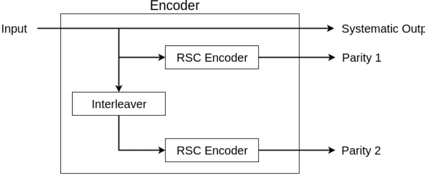
Figure 3.3: An example of a turbo code encoder containing two RSC encoders.
3.1.1 Turbo Code Encoder
Turbo code encoding at the lowest level uses a Recursive Systematic Convolutional
(RSC) encoder. An example is shown in Figure 3.2. An RSC encoder takes an input
sequence of bits and produces two output sequences of bits of equal length. One
sequence exactly matches the input sequence, known as the systematic bits, and the
other sequence is the parity bits, or redundant information used to help recover the
input sequence. The recursive aspect of RSC encoders uses a feedback which creates
[image:27.612.107.526.300.473.2]Figure 3.4: A high level view of the turbo code decoder consisting of MAP decoders, interleavers, deinterleavers, and a hard decision maker. The bold lines highlight the feedback loop present in the turbo decoder.
will continue to have the parity bits change even if in the presence of a long string of
the same bit values which is beneficial for error correction.
Multiple RSC encoders can be concatenated in parallel to increase the amount
of parity information. In order to decorrelate the redundancy bits from the two
encoders, an interleaver is used at the input of the second RSC encoder to change
the order of the bits. This is done for each subsequent RSC encoder. The additional
RSC encoders systematic outputs do not provide new information and are ignored.
An example turbo code encoder with two RSC encoders can be seen in Figure 3.3.
This example encoder is used for the remainder of this section.
3.1.2 Turbo Code Decoder
In this example the turbo code decoder contains two Maximum A Posteriori (MAP)
decoders, otherwise called Bahl, Cocke, Jelinek, and Raviv (BCJR) decoders [24].
Each MAP decoder is used for one parity sequence.
The outputs of the MAP decoders are used as inputs to the subsequent decoders
Figure 3.5: The state machine representing the example RSC encoder. The encoder memory is shown in the parenthesis. Inputs of zero are shown as dotted lines, and inputs of one are shown with full lines. The input and output format is represented as input/output marked on the transition lines.
Figure 3.6: This diagram represents a trellis with 5 states over 4 bits. The red lines
[image:29.612.109.542.402.670.2]increases so does the confidence in the output. When the desired number of iterations
through the feedback loop is met, both outputs are fed into a hard decision maker
which gives the final output.
The MAP decoder makes up the complex part of this algorithm. It constitutes
the majority of the decoder, and relies heavily on the trellis structure. A trellis is a
time-invariant state machine used to represent an RSC encoder. The truth table for
every possible state for the previous RSC encoder can be seen in Table 3.1. A state
machine can be extracted from this truth table. The state machine representation
can be seen in Figure 3.5. The RSC encoder used has a memory of two bits, or four
possible states, as seen in the figure. This state machine over time makes up the
trellis. The trellis used for this example can be seen in Figure 3.6. Examining the
figure shows the four states at each time interval, along with the transitions between
each time interval. When encoding, a single path is taken through the trellis, where
a new parity bit is produced at each step. An example of this is displayed through
Figure 3.7. The MAP decoder uses this trellis structure which represents how the
input sequence was encoded, and tries to find the path taken using the systematic
sequence and the parity sequence.
The MAP decoder calculates the Log Likelihood Ratio (LLR) for each bit, or in
other words the probability a bit is a 0 or a 1. The LLR is calculated as
LLR(uk|y) = log
P(uk = 1|y)
P(uk = 0|y)
, (1)
here P(uk = 1|y) is the probability that the bit uk is 1 given the entire information
sequence, y, has been received and where P(uk = 0|y) is the probability that the
Table 3.1: Truth table representation of the RSC encoder shown previously.
Input Memory 1 Memory 2 State A = Memory 1
XOR Memory 2
B = Input XOR A
Output = Memory 2 XOR B
0 0 0 0 0 0 0
0 0 1 1 1 1 0
0 1 0 2 1 1 1
0 1 1 3 0 0 1
1 0 0 0 0 1 1
1 0 1 1 1 0 1
1 1 0 2 1 0 0
1 1 1 3 0 1 0
0 0 0 0 0 0 0
0 0 1 1 1 1 0
0 1 0 2 1 1 1
0 1 1 3 0 0 1
1 0 0 0 0 1 1
1 0 1 1 1 0 1
1 1 0 2 1 0 0
1 1 1 3 0 1 0
expressed using three terms as follows
LLR(uk|y) = ln
P
(αk−1(s0)γ(s0, s)βk(s))
P
(αk−1(s0)γ(s0, s)βk(s))
, (2)
where αk−1(s0) is the probability that the trellis is in state s0 at t = k −1, starting
fromt= 0 and moving forward in time, whereβk(s) is the probability that the trellis
is in state s at t = k, starting from t = N and moving backwards in time, and
where γk(s0, s) is the probability that if the trellis is in state s0 at time t =k−1, it
moves to state s att =k. The γ terms are branch transition probabilities known as
the branch metrics. The α terms are computed recursively moving forward in time,
called forward recursion, and theβ terms are computed recursively moving backward
in time, called backward recursion.
Figure 3.8: This diagram shows how the Gamma, Alpha, and Beta terms are represented in the trellis. The Gamma terms are the state transitions represented by the Γn in the
diagram. The Alpha terms are denoted byAn and move left to right. The Beta terms are
denoted by BN and move right to left.
Figure 3.8 displays each of the terms by labeling pieces of the trellis. In the figure the
gamma terms are represented by the transitions between the states, while the Alpha
terms are represented by the states going forward, and the Beta terms are represented
by the states going backwards.
The branch metrics or gamma terms are calculated
γk(s0, s) =Ckexp (
1
2(Lcykuk+ukL(uk) +Lc
n
X
i=1
ykixki)), (3)
where uk is the trellis input, L(uK) is the extrinsic information from the previous
MAP decoder, Lc is the channel reliability, n is the number of bits being considered
bit or parity bit), xk is the trellis output, and Ck is a constant that gets divided out
later and can be ignored.
The forward recursion or alpha terms are calculated
αk(s) = αk−1(s0)γk(s0, s), (4)
where α0 is initialized
α0(s) =
1, if s= 0
0, otherwise.
The backward recursion or beta terms are calculated
βk−1(s)) =βk(s0)γk(s0, s), (5)
where βk−1 is initialized
βk−1(s) =
1, if s= 0
0, otherwise.
The MAP decoding algorithm requires long, resource intensive exponential
func-tions, and a large number of multiplication functions. Improvements using the log
domain can greatly reduce the complexity without sacrificing any accuracy [10].
Us-ing the log domain, exponentials can be removed, the large amount of multiplications
can become additions, and additions can become the max* operation seen in equation
3.
max∗(a, b) = max(a, b) +ln(1 +e−|a−b|), (6)
This variation is commonly referred to as the MAX-LOG-MAP algorithm. Further
simplifications can be made while still maintaining exceptional results by using the
a small 8 value look up table[25]. The decoder can be simplified even further by
ignoring the correction factor entirely. This is commonly referred to as the
MAX-MAP algorithm. For simplicity, the MAX-MAX-MAP variant of the algorithm was used
for the FPGA acceleration.
The Γ terms in the log domain can be computed as follows
Γk(s0, s) =
1
2ukL(uk) +
Lc
2
n
X
i=1
ykixki (7)
The alpha terms in the log domain can be computed as follows
log(αk(s)) =Ak(s) = max∗
s0 (Ak−1(s
0
) + Γk(s0, s)), (8)
where A0 is initialized
A0(s) =
0, if s= 0
−∞, otherwise.
The beta terms in the log domain can be computed as follows
log(βk−1(s)) =Bk−1(s) = max∗
s0 (Bk(s
0
) + Γk(s0, s)), (9)
where Bk−1 is initialized
Bk−1(s) =
0, if s= 0
−∞, otherwise.
Upon completion of all of three of these terms, the extrinsic information or LLR
can be calculated in the log domain as
L(uk|y) = max∗
(s0,s)foruk=1(Ak−1(s
0
− max∗
(s0,s)foruk=0(Ak−1(s
0) + Γ
k(s0, s) +Bk(s)), (10)
Again, this extrinsic information is used in subsequent decoders to improve the
reli-ability of the error correction.
The outputs of the MAP decoders are fed to the hard decision maker.
uk =
1, if L(uk|y)1+L(uk|y)2+Lc∗uk >0
0, otherwise.
The two outputs are added together along with the systematic bit multiplied by the
channel reliability. If the value is positive it is considered a 1 otherwise it is a zero.
The equation can be seen in the Equation above.
3.1.3 Implementations
There are many variants of the MAP decoder which have implementation
advan-tages. Each of the variants were implemented one by one. Initially, the regular
MAP decoder was implemented in software. The psuedocode for the MAP decoder
can be seen in Appendix A. Then the LOG-MAP implementation was created,
fol-lowed by the MAX-LOG-MAP implementation, MAX-LOG-LUT-MAP, and finally
the MAX-MAP implementation. The LOG-MAP variant is the same as the MAP
decoder but using the log domain. The MAX-LOG-MAP decoder is the same as the
LOG-MAP decoder but uses the max* operator in place of the log function. The
MAX-LOG-LUT-MAP is the same as the MAP-LOG-MAP but uses a look up table
for the correction factor in place of calculating the max* correction factor. Finally,
the MAX-MAP is the same as the MAX-LOG-LUT-MAP but ignores the correction
factor entirely. The psuedocode for the MAX-MAP decoder can be seen in appendix
B.
research. Supporting code was written to test the turbo code decoder, including the
different variants of the MAP decoder. This code produced random sequences of
data, created interleaver patterns used for encoding and decoding of data, encoded
the data using the turbo code encoder, added Gaussian noise to the signal, ran the
turbo code decoder, recorded the decoding time, calculated the BER of the output,
and printed the results with their corresponding input parameters. The block size
and trellis size were compile time macros, but the testing framework allowed simple
iterations through some run time parameters as well. The SNR start, stop, and step
amounts, the number of turbo decoder iteration start, stop, and step amounts, and
the number of simulations per parameter were all run time specified, allowing for
many parameters to be checked in a single run. The turbo code decoder using the
MAX-MAP decoder results can be seen in Figure 3.9. This figure clearly shows that
performance of the error correction improves with increased iterations and approaches
High Level Synthesis Guidelines
The goal of HLS tools is to facilitate the design process of hardware implementations
on the FPGA by translating a software description of an algorithm into a hardware
description language implementation. Taking software designed for sequential
exe-cution will likely not produce hardware implementations that are competitive with
the ideal manually optimized designs. Instead, to maximize the effectiveness when
utilizing HLS tools, it is important to take special care in the design approach, and to
develop the software implementation with a hardware-centric mindset. This involves
starting with a hardware design in mind and writing code that attempts to emulate
it. Additionally, it involves adapting the coding style to the HLS requirements, which
is not always in agreement with software best practices. In this work, important
aspects of this design process are identified in order to use the HLS tool effectively.
One of the goals of this research was to identify the necessary aspects of HLS that
lead to hardware comparable in terms of performance to manually optimized designs.
Three different points of interest were identified to be very important and can be seen
as guidelines that lead to good implementation.
1. A good understanding of the tools.
2. Having a coding style that is effective for HLS.
emulate it.
This section will discuss these point at a general level and provide some examples.
After this, the implementation of the algorithm is discussed in detail.
4.1
Understand The Tool Offerings
An understanding of what is offered from the tools, and how the tools work in terms
of synthesis, are essential elements necessary to take advantage of HLS. In the case
of Vivado HLS that means understanding the available implementation choices such
as directives, data types, and interfaces, and when to use them. It also means being
able to read and understand HLS reports, and being able to analyze the output using
the different analysis tools provided.
4.1.1 IDE Features
Vivado HLS has many features that can greatly enhance productivity and shorten
development time. Some of these features include analysis tools which explain the
mapping between the high level code and cycle by cycle operation, resource usage,
timing information, and different simulation methods.
4.1.2 Directives
Arguably the most significant aspect of Vivado HLS to understand is the directives.
As mentioned previously, using HLS to compete with hand coded RTL
implemen-tations is not as simple as selecting a function to synthesize. Part of the reasoning
behind this is that there are many things that can be done in hardware that cannot
be expressed in high level code alone. To accommodate for this HLS tools can be
provided with directives. Directives are extensions of C and C++ that guide the
very impactful in HLS hardware designs, and thus greatly affecting performance and
resource utilization:
• Pipelining directive allows fine grained parallelism by increasing utilization of
hardware. It is used to pipeline loops, allowing future iterations of for loops to
start before the previous ones have finished, increasing utilization and
through-put. Pipelining isn’t always free however. When pipelining a loop, all sub loops
and sub functions may be unrolled completely which can dramatically increase
resource usage.
• Dataflow directive allows coarse grained parallelism across functions or loops
which increasing utilization of hardware. Dataflow will place a FIFO buffer
between functions or between loops enabling subsequent functions or loops to
receive and work with data before the previous function or loop has finished.
• Loop unrolling allows parallelism in loops by replicating hardware. This can be
very effective, allowing single cycle computations, but can be costly in terms of
resources.
• Array partitioning reduces access contention by splitting an array at the
hard-ware level, which provides more parallel ports for access. The Array Partitioning
directive requires intimate knowledge of the hardware design, and data access
patterns, but without it severe penalties can be faced. For large arrays, block
RAM is most commonly used as storage. Although this is often the appropriate
method to use, block RAM only has two ports per block that can be used data
access each cycle. This can be a huge bottleneck in a design. Partitioning splits
the arrays among different blocks, allowing for more ports to access the memory
at once. Arrays can be partitioned completely allowing for fully parallel access,
• Inlining removes the hierarchy of the function call which in turn allows the
tools more freedom to optimize. This can be quite effective for increasing
per-formance, but can be more confusing for analysis.
• Interface specifies how the ports are created. This is a very significant directive
when it comes to system integration as it directs how the data is passed into
and out of the accelerator, and how it is interacted with.
• Dependence provides the tools with more information enabling false
dependen-cies to be removed, which allows pipelining or improved pipelining. The tools
choose functionality over performance and thus sometimes see dependencies
that are not required. Eliminating those false or not required dependencies can
enhance pipelining performance.
4.1.3 Data Types and Libraries
Xilinx provides arbitrary precision libraries which let the user have more control
over data types. With these libraries a user can select the bit widths of data types,
which can be very useful for minimizing resources, or creating data types larger than
can be specified using native C or C++ types. These libraries are also useful for
implementing fixed point data types. Fixed point data types are common in hardware
designs as replacements for floating point as they can be calculated much faster and
more efficiently.
In addition to that there are also other libraries provided by Xilinx that can be
leveraged for effective implementations. Some of these libraries include DSP, Math,
4.2
Coding Style
When writing the code for the hardware it is important to have a coding style tailored
to hardware. In other words, when implementing a design it is best not to have a
software perspective in mind, but instead think about what hardware will be created
from the high level code. For example in software, it is good practice to avoid branches
when possible as branch penalties can play a huge factor in slowing performance.
Branches behave differently when consider for HLS. Using HLS, an if statement
will usually be interpreted as a multiplexor in hardware. Multiple multiplexors or
larger multiplexors do not face the same penalties as branch penalties. It is this
kind of thinking, and understanding of what hardware the tools will interpret from
the code that will guide good coding style and implementations. This can be a
difficult mindset to adjust to at first, but is vital for good results. Along with this,
there are many restrictions on coding styles as some things are not synthesizable.
Some of the unsynthesizable aspects include operating system calls, STL functions,
function pointers, and pointers without compile time size definitions. In addition to
this recursion is not allowed, and pointer casting is very limited.
There are several ideas that come to mind for guiding good code. Code should be
explicit and well defined. The tools will not optimize the hardware unless it can prove
optimization will not break functionality. Being explicit provides more information
and allows more optimizations to occur. Also keeping the control flow simple and
avoiding complex code will produce better results. More complex control flow leads
to higher resource usage requirements as well as longer latency delays. Understanding
the building block of the FPGA such as FlipFlops, LUTs, DSP48s, or block RAM,
and coding to take advantage of their properties can be beneficial as well.
A few examples taken from [26] of how to take advantage of these ideas in coding
4.2.1 Bounded Loop Iterators
Bounding loops with a maximum number of iterations and using break statements
for early termination will allow the tools to run optimizations that arent possible
with dynamic for loops. Again the tools do not break functionality, so if a variable is
specified as an 32 bit int but it only ever loops a maximum of 200 times, depending
on how its written, the tools may not be able to prove that the counter never goes
over 200 and thus will unnecessarily use 32 bit variables to count. These longer 32
bit variables take up more resources and take longer to evaluate than 8 bit variables.
With perfectly defined loops the bit widths of the data path and control signals can
be optimized.
Listing 4.1: Example code which does not provide definitive boundaries for the for loop
resulting in subpar HLS results.
1 # define MAX 200
2 int total(int in_array[MAX] , int size){
3 int total=0;
4 for(int i=0; i<size; i++){
5 total = total + in_array[i] ;
6 }
7 return total;
8 }
Listing 4.2: Example code with bounded loops and an early conditional break statement
which allows the HLS to optimize the implementation.
1 # define MAX 200
2 int total(int in_array[MAX] , int size){
4 for(int i=0; i<MAX; i++){
5 total = total + in_array[i] ;
6 if (i == size) {
7 break;
8 }
9 }
10 return total;
11 }
4.2.2 Being Explicit Where Possible
This bring about the point of being explicit and allowing the tools to make
optimiza-tions. For example, although the tools will interpret if statements as multiplexors,
it does not mean if statements should be used without consideration. The tools
will optimize where possible by sharing resources. In the example below there are
two if statements that could be written using if else instead. Using two separate if
statements will duplicate the foo hardware as the tools cannot prove the paths are
mutually exclusive. Figure 4.1 shows a simplified idea of potential hardware that
could be created from the description. As can be seen in the figure, the foo hardware
is duplicated.
Listing 4.3: Example code disregarding potential mutual exclusion which restricts the
tools from optimizing.
1 if (A == Value1)
2 A = Foo(X) ;
3 if (B == Value2)
4 B = Foo(Y) ;
Figure 4.2: Illustration of the hardware interpretation when mutual exclusion is proven. In this case one foo unit can be shared.
The following listing provides more information that can be taken advantage of
to enhance hardware implementation. A simplified idea of the hardware that could
be created from this high level code can be seen in Figure 4.2. This figure has a more
complicated control path but enables a single foo hardware unit to be implemented
which may be very beneficial.
Listing 4.4: Example code being explicit and displaying mutual exclusion which allows
the tools to optimize further. In this case by sharing resources.
1 if (A == Value1)
2 A = Foo(X) ;
3 else if (B == Value2)
4 B = Foo(Y) ;
Written this way, mutual exclusion is proven, and resource sharing optimizations
applied more widely in design.
4.2.3 Single Return Point
Another good design practice is using a single return point. This can lower the
complexity of the control path, and allows for the pipeline stages to be balanced
better. This is beneficial for resource usage, latency, and debugging. If there is
more than one possible exit point, flags can be used to skip extra computation. The
example below first shows code that can return early which should try to be avoided
for HLS. After this an alternative method of using flags is shown.
Listing 4.5: Example code showing multiple return points in a function which should be
avoided for good HLS coding style.
1 if (exit_early == true) {
2 return A;
3 }
4 A = A + B;
5 return A;
Listing 4.6: Example code showing how flags can be used to easily bypass sections of code
and cleanly create a single return point.
1 flag_add_B = true;
2 if (exit_early == true) {
3 flag_add_B = false;
4 }
5 if (flag_add_B == true) {
6 A = A + B;
7 }
Although this code can be simplified further, the coding style of using flags to
bypass sections of code has shown to be effective for more complex examples.
4.3
Write Code That Emulates Hardware
One of the most significant aspects for HLS implementations that achieve near hand
coded performance is writing code that tries to emulate a hardware design. This
is very important as this type of coding doesn’t always make sense from a software
standpoint but is vital for good results. Software that achieves the same functional
equivalency can likely be completed in a more straightforward implementation with
fewer lines of code, but gives very different hardware results. For example increasing
parallelism at the hardware level can lead to code which has a complex control flow,
and calls the same function multiple times, which has no software benefit.
Addition-ally, this may introducing extra variables or extra buffers that are unnecessary in
software.
One example of this can be seen in a simplified case that was encountered through
this work. In this case, dataflow and pipelining were not applicable due to the nature
of the dependencies. The software functionality is capable of being expressed as shown
in the listing below. The subsequent hardware created can be seen in Figure 4.3. The
figure demonstrates how the code will produce hardware that runs sequentially.
Listing 4.7: Example code showing how hardware performance can be limited due to data
dependencies on a single buffer.
1 for (LOOP) {
2 ACQUIRE_DATA(A) ;
3 USE_DATA(A) ;
Figure 4.3: Example of resulting hardware from listing 4.7
occur in parallel to increase performance. To do this, a pingpong buffer scheme
could be used. In this case, the acquire data function would use one buffer, while
the use data buffer would use another buffer, and they would swap buffers for each
loop. Code to represent this hardware can be seen in the listing below. The hardware
representing of this can be seen in Figure 4.4. This figure clearly shows the two
functions can run in parallel by removing the dependencies between them.
Listing 4.8: Example code showing how parallel functions could be used to reduce the
memory access limitations.
1 // I n i t i a l i z a t i o n
2 ACQUIRE_DATA(B) ;
3 Toggle = true;
4
Figure 4.4: Example of resulting hardware from listing 4.8
6 if Toggle {
7 ACQUIRE_DATA(A) ;
8 USE_DATA(B) ;
9 }
10 else {
11 ACQUIRE_DATA(B) ;
12 USE_DATA(A) ;
13 }
14 Toggle = !Toggle;
15 }
16 // c l e a n u p
As can be seen when comparing both code listings, the pingpong buffer scheme
adds complexity to the code which would not add any benefit during software
ex-ecution. The hardware on the other hand would be significantly different, gaining
the ability for the functions to occur in parallel. This is only a simple example, but
HLS MAX-MAP Implementation
The turbo code decoder is the complex part of turbo code error correction. Within
the turbo code decoder, the complex, compute intensive piece of the algorithm is
the MAP decoder. This was chosen to undergo FPGA acceleration. In this case,
the MAX-MAP variant of the MAP decoder described previously, was used as it
contains many benefits for hardware implementation. This chapter describes the
implementation details of the MAX-MAP decoder for targeting HLS. The high level
hardware designs are explored first, followed by the low level building blocks that
made up the implementation.
5.1
High Level Designs
The explanation of the implementation is easiest to comprehend from the top-down,
looking at the high level design approach. Furthermore, starting with the software
implementation, and moving through the hardware designs provides insight into the
thought process that was behind the implementations, and demonstrates the ability
to easily explore the design space. Ultimately, there were three different hardware
designs that were created, building off what was learned from previous
Figure 5.1: The high level flow of data for the original MAP decoder. The N inputs rep-resents the entire block of information received. Each of the terms are calculated separately in their entirety before continuing to the next calculations.
5.1.1 Software
At the topmost level, the block diagram software implementation can be seen. The
regular software flow of data through a MAX-MAP decoder can be seen in Figure
5.1. This figure shows the algorithm being broken down into 4 main functions, each
one representing one of the terms of the algorithm. In this implementation, each of
these calculations occurs for the entire N inputs, which typically ranges from 40 to
6144 as specified in the LTE standard [27], before starting the next calculations. This
requires the entire input block to be received before continuing, and requires all of
Listing 5.1: Pseudo Code for the original software design.
1 MAP_decode(systematic[NUM_BITS] ,
2 parity[NUM_BITS] ,
3 extrinsic[NUM_BITS] ,
4 noise,
5 decoder_output[NUM_BITS] )
6 {
7 calculate_gamma(systematic[NUM_BITS] ,
8 parity[NUM_BITS] ,
9 extrinsic[NUM_BITS] ,
10 noise,
11 gamma_output[NUM_BITS] ) ;
12
13 calculate_alpha(gamma_output, alpha_output) ;
14
15 calculate_beta(gamma_output, beta_output) ;
16
17 calculate_LLR(gamma_output,
18 alpha_output,
19 beta_output,
20 decoder_output) ;
21 }
5.1.2 Hardware Design 1: Initial Sliding Window
The target hardware implementation for HLS uses a sliding window approach, which
is common for hardware designs. In this case, a sliding window approach means only
a number of bits are considered at one time, starting with the first bits and moving
to the later bits, rather than using the entire sequence at once. A visual example
of this using a trellis structure can be seen in Figure 5.2. Other than allowing for
Figure 5.2: The sliding window approach shown on a trellis structure. In this example a window of 5 and a hop of 2 is used.
the algorithm itself. On one hand, the Beta values can start to be calculated before
all of the bits are received, and thus before all the Gamma and Alpha calculations
are completed. Because of this, continuous streams of data are possible, instead
of requiring whole blocks at a time. Additionally, this approach allows for more
parallelism, and less resource usage as less information is needed at one time. This
approach is made possible by initializing the Beta values with either equal probability
of being in each state, or the most recently calculated Alpha values for each state.
This design takes a slight hit in accuracy as the starting state of the Beta values is
unknown. To reduce the effect of this imperfect initialization, the first Beta values
calculated are thrown away as they are not as accurate as the later values. They are
recalculated again later, requiring extra
The high level design of the sliding window implementation can be seen in Figure
5.3. It is important to note that the figure ignores the initialization and cleanup
re-quired for the sliding window approach, but is rere-quired for the actual implementation.
A significant aspect to the design is that to reduce the number of extra calculations,
instead of having the window slide and produce one output per frame, it hops by
nested loops inside of it. Each iteration will produce H results, while N/H iterations
will produce outputs for all of the N inputs. In this design, the Gamma and Alpha
Calculation Units are combined as they can occur concurrently. These terms do not
require any extra calculations and thus loop H times. The results are then stored in
a buffer, where the Gamma results are passed to the the Beta Calculation hardware.
The Beta Calculation require the extra calculations and thus loops W times, using
only H results for the next hardware. The extrinsic values are then calculated using
all three buffers. This hardware loops H times and produces one output per loop.
Only the last H calculated Beta values are used in the extrinsic value calculation.
Listing 5.2: Pseudo Code for the original sliding window design.
1 MAP_decode(systematic[NUM_BITS] ,
2 parity[NUM_BITS] ,
3 extrinsic[NUM_BITS] ,
4 noise,
5 decoder_output[NUM_BITS] )
6 {
7
8 /∗ ∗ ∗ ∗ ∗ ∗ ∗ ∗ ∗ ∗ ∗ ∗ ∗ ∗ ∗ ∗ ∗ ∗ ∗ ∗ ∗ ∗ ∗ ∗ ∗ ∗ ∗ ∗ ∗ ∗ ∗ ∗ ∗ ∗ ∗ ∗ ∗ ∗ ∗ ∗ ∗
9 i n i t i a l i z a t i o n c o d e
10 ∗ ∗ ∗ ∗ ∗ ∗ ∗ ∗ ∗ ∗ ∗ ∗ ∗ ∗ ∗ ∗ ∗ ∗ ∗ ∗ ∗ ∗ ∗ ∗ ∗ ∗ ∗ ∗ ∗ ∗ ∗ ∗ ∗ ∗ ∗ ∗ ∗ ∗ ∗ ∗ ∗/
11
12 for NUM_BITS/WINDOW_HOP {
13
14 // C a l c u l a t e t h e new gamma and a l p h a g o i n g f o r w a r d s i n t i m e
15 for WINDOW_HOP {
16 //PIPELINE
17 # pragma HLS p i p e l i n e I I=xx
18 new_gamma = calculate_gamma(systematic[bit] , parity[bit] , ←
19 bit++;
20 gamma_buffer_write(new_gamma) ;
21
22 new_alpha = calculate_alpha(last_alpha, gamma_buffer, ←
-trellis) ;
23 alpha_buffer_write(new_alpha) ;
24 last_alpha = new_alpha;
25 }
26
27 // C a l c u l a t e b e t a t e r m s g o i n g b a c k w a r d s i n t i m e
28 // i n i t i a l i z e from t h e l a s t c a l c u l a t e d a l p h a
29 last_beta = last_alpha;
30
31 //Go t h r o u g h t h e e n t i r e window l e n g t h f o r t h e Beta t e r m s
32 for WINDOW {
33 //PIPELINE
34 # pragma HLS p i p e l i n e I I=xx
35 new_beta = calculate_beta(last_beta, gamma_buffer, trellis←
-) ;
36 beta_buffer_write(new_beta) ;
37 last_beta = new_beta;
38 }
39
40 // C a l c u l a t e E x t r i n s i c LLRs
41 for WINDOW_HOP {
42 //PIPELINE
43 # pragma HLS p i p e l i n e I I=xx
44 result = calculate_extrinsic(gamma_buffer, alpha_buffer, ←
-beta_buffer, trellis) ;
45 decoder_output_write(result) ;
46 }
47 } // END f o r NUM BITS/WINDOW HOP
49 /∗ ∗ ∗ ∗ ∗ ∗ ∗ ∗ ∗ ∗ ∗ ∗ ∗ ∗ ∗ ∗ ∗ ∗ ∗ ∗ ∗ ∗ ∗ ∗ ∗ ∗ ∗ ∗ ∗ ∗ ∗ ∗ ∗ ∗ ∗ ∗ ∗ ∗ ∗ ∗ ∗
50 c l e a n u p c o d e
51 ∗ ∗ ∗ ∗ ∗ ∗ ∗ ∗ ∗ ∗ ∗ ∗ ∗ ∗ ∗ ∗ ∗ ∗ ∗ ∗ ∗ ∗ ∗ ∗ ∗ ∗ ∗ ∗ ∗ ∗ ∗ ∗ ∗ ∗ ∗ ∗ ∗ ∗ ∗ ∗ ∗/
52 }
Special buffers were necessary and are explicitly shown in this design. The buffers
only hold one window size of data. This enables the hardware design to use much
less resources than storing the entire block of all the terms.
From the analysis of our design, unsurprisingly, the Beta calculations took most
computation time. This is due to the multiple times more calculations being required
than the Gamma and Alpha calculations. Two different directions were explored from
this point.
5.1.3 Hardware Design 2: Replicated Hardware
The second design, shown in Figure 5.4, sought to alleviate the Beta Calculation Unit
bottleneck by replicating hardware, enabling parallel Beta Calculation Units. This
effectively hides the extra calculations. To accommodate for this approach, larger
buffers are required, as well as extra resources for the duplicated hardware. Still,
with this design only a single type of calculation unit could run at one time.
In this case, there are nB Beta Calculation Units. This requires nB times the
amount of new data to work with each loop. For this reason, the Gamma and Alpha
Calculation Units loop nB times as the previous version, represented by nB*H in
the figure. The individual Beta Calculation loops remain at W loops as they are
independent. Again nB times the amount of data per loop will be produced, requiring
the LLR Calculation Unit to loop nB times as the previous version as well, represented
by nB*H in the figure. As the inner loops is going through nB times as much data
per loop, the outer loop needs to run fewer times to handle the same amount of data
Listing 5.3: Pseudo Code for the second sliding window design with two Beta Calculation
Units.
1 MAP_decode(systematic[NUM_BITS] ,
2 parity[NUM_BITS] ,
3 extrinsic[NUM_BITS] ,
4 noise,
5 decoder_output[NUM_BITS] )
6 {
7
8 /∗ ∗ ∗ ∗ ∗ ∗ ∗ ∗ ∗ ∗ ∗ ∗ ∗ ∗ ∗ ∗ ∗ ∗ ∗ ∗ ∗ ∗ ∗ ∗ ∗ ∗ ∗ ∗ ∗ ∗ ∗ ∗ ∗ ∗ ∗ ∗ ∗ ∗ ∗ ∗ ∗
9 i n i t i a l i z a t i o n c o d e
10 ∗ ∗ ∗ ∗ ∗ ∗ ∗ ∗ ∗ ∗ ∗ ∗ ∗ ∗ ∗ ∗ ∗ ∗ ∗ ∗ ∗ ∗ ∗ ∗ ∗ ∗ ∗ ∗ ∗ ∗ ∗ ∗ ∗ ∗ ∗ ∗ ∗ ∗ ∗ ∗ ∗/
11
12 for NUM_BITS/ (WINDOW_HOP∗NUM_BETA_CALCULATION_UNITS) {
13
14 // C a l c u l a t e t h e new gamma and a l p h a g o i n g f o r w a r d s i n t i m e
15 for WINDOW_HOP∗NUM_BETA_CALCULATION_UNITS {
16 //PIPELINE
17 # pragma HLS p i p e l i n e I I=xx
18 new_gamma = calculate_gamma(systematic[bit] , parity[bit] , ←
-extrinsic[bit] , noise_param, trellis) ;
19 bit++;
20 gamma_buffer_write(new_gamma) ;
21
22 new_alpha = calculate_alpha(last_alpha, gamma_buffer, ←
-trellis) ;
23 alpha_buffer_write(new_alpha) ;
24 last_alpha = new_alpha;
25 }
26
27 // C a l c u l a t e b e t a t e r m s g o i n g b a c k w a r d s i n t i m e
29 last_beta = last_alpha;
30
31 //Go t h r o u g h t h e e n t i r e window l e n g t h f o r t h e Beta t e r m s
32 for WINDOW {
33 //PIPELINE
34 # pragma HLS p i p e l i n e I I=xx
35 new_beta1 = calculate_beta(last_beta1, gamma_buffer, ←
-trellis) ;
36 beta_buffer1_write(new_beta1) ;
37 last_beta1 = new_beta1;
38
39 new_beta2 = calculate_beta(last_beta2, gamma_buffer, ←
-trellis) ;
40 beta_buffer2_write(new_beta2) ;
41 last_beta2 = new_beta2;
42 }
43
44 // C a l c u l a t e E x t r i n s i c LLRs
45 for WINDOW_HOP {
46 //PIPELINE
47 # pragma HLS p i p e l i n e I I=xx
48 result1 = calculate_extrinsic(gamma_buffer, alpha_buffer, ←
-beta_buffer1, trellis) ;
49 decoder_output_write(result1) ;
50
51 result2 = calculate_extrinsic(gamma_buffer, alpha_buffer, ←
-beta_buffer2, trellis) ;
52 decoder_output_write(result2) ;
53 }
54 } // END f o r NUM BITS/WINDOW HOP
55
56 /∗ ∗ ∗ ∗ ∗ ∗ ∗ ∗ ∗ ∗ ∗ ∗ ∗ ∗ ∗ ∗ ∗ ∗ ∗ ∗ ∗ ∗ ∗ ∗ ∗ ∗ ∗ ∗ ∗ ∗ ∗ ∗ ∗ ∗ ∗ ∗ ∗ ∗ ∗ ∗ ∗
Figure 5.5: The third high level hardware design. This design also has parallel Beta Calculation Units but is different in that the entire design is pipelined instead of just the inner loops so each of the calculation units have the ability to run in parallel. In this diagram nB represents the number of parallel Beta Calculation Units, N represents the number of inputs in the block, W represents the number of inputs in the window, and H represents the amount to hop by for each window.
58 ∗ ∗ ∗ ∗ ∗ ∗ ∗ ∗ ∗ ∗ ∗ ∗ ∗ ∗ ∗ ∗ ∗ ∗ ∗ ∗ ∗ ∗ ∗ ∗ ∗ ∗ ∗ ∗ ∗ ∗ ∗ ∗ ∗ ∗ ∗ ∗ ∗ ∗ ∗ ∗ ∗/
59 }
5.1.4 Hardware Design 3: Fully Pipelined
A key feature of any hardware design is to utilize the hardware as much as possible.
One limitation of the second d