White Rose Research Online
eprints@whiterose.ac.uk
Universities of Leeds, Sheffield and York
http://eprints.whiterose.ac.uk/
This is the author’s post-print version of an article published in
Climate
Dynamics, 37 (7-8)
White Rose Research Online URL for this paper:
http://eprints.whiterose.ac.uk/id/eprint/77217
Published article:
Sedlar, J, Tjernstrom, M, Mauritsen, T, Shupe, MD, Brooks, IM, Persson, POG,
Birch, CE, Leck, C, Sirevaag, A and Nicolaus, M (2011)
A transitioning Arctic
surface energy budget: the impacts of solar zenith angle, surface albedo and
cloud radiative forcing.
Climate Dynamics, 37 (7-8). 1643 - 1660. ISSN
0930-7575
(will be inserted by the editor)
A transitioning Arctic surface energy budget: the impacts
of solar zenith angle, surface albedo and cloud radiative
forcing
Joseph Sedlar · Michael Tjernstr¨om ·
Thorsten Mauritsen · Matthew D. Shupe ·
Ian M. Brooks · P. Ola G. Persson · Cathryn
E. Birch · Caroline Leck · Anders Sirevaag ·
Marcel Nicolaus
Received: date / Accepted: date
Abstract Snow surface and sea-ice energy budgets were measured near 87.5N dur-ing the Arctic Summer Cloud Ocean Study (ASCOS), from August to early Septem-ber 2008. Surface temperature indicated 4 distinct temperature regimes, characterized by varying cloud, thermodynamic and solar properties. An initial warm, melt-season regime was interrupted by a 3-day cold regime where temperatures dropped from near zero to -7◦C. Subsequently mean energy budget residuals remained small and near
zero for 1 week until once again temperatures dropped rapidly and the energy budget residuals became negative. Energy budget transitions were dominated by the net
ra-J. Sedlar
Department of Meteorology, Stockholm University, Stockholm, Sweden Tel.: +46-816-2534
E-mail: josephs@misu.su.se M. Tjernstr¨om
Stockholm University, Stockholm, Sweden T. Mauritsen
Max Planck Institute for Meteorology, Hamburg, Germany M. D. Shupe
University of Colorado and NOAA-ESRL-PSD, Boulder, CO, USA I. M. Brooks
University of Leeds, Leeds, UK P. O. G. Persson
University of Colorado and NOAA-ESRL-PSD, Boulder, CO, USA C. E. Birch
University of Leeds, Leeds, UK C. Leck
Stockholm University, Stockholm, Sweden A. Sirevaag
University of Bergen and Bjerknes Center for Climate Research, Bergen, Norway M. Nicolaus
diative fluxes, largely controlled by the cloudiness. Variable heat, moisture and cloud distributions were associated with changing air-masses.
Surface cloud radiative forcing, the net radiative effect of clouds on the surface relative to clear skies, is estimated. Shortwave cloud forcing ranged between -50 W m−2and zero and varied significantly with surface albedo, solar zenith angle and cloud liquid water. Longwave cloud forcing was larger and generally ranged between 65-85 W m−2, except when the cloud fraction was tenuous or contained little liquid water; thus the net effect of the clouds was to warm the surface. Both cold periods occurred under tenuous, or altogether absent, low-level clouds containing little liquid water, effectively reducing the cloud greenhouse effect. Freeze-up progression was enhanced by a combination of increasing solar zenith angles and surface albedo, while inhibited by a large, positive surface cloud forcing until a new air-mass with considerably less cloudiness advected over the experiment area.
Keywords Arctic · Sea ice · Surface energy budget · Cloud radiative forcing ·
Shortwave radiation·Longwave radiation
1 Introduction
The Arctic has become a focal point for studying the Earth’s response to a changing climate (e.g. ACIA 2005; Overland et al 2008; Overland 2009), as it has witnessed amplified surface warming by roughly a factor of two compared to the global average (ACIA 2005; IPCC 2007), as well as warming aloft (Graversen et al 2008). A central focus is on the reduction of the perennial sea-ice (e.g. Lindsay and Zhang 2005; Serreze et al 2007; Overland 2009), especially since the record ice-loss of 2007 (e.g. Kay et al 2008; Zhang et al 2008a; Lindsay et al 2009). The debate over the primary forcings responsible for Arctic climate changes is reflected in the literature: Changes in the large-scale atmospheric circulation patterns (eg. Graversen 2006; Graversen et al 2008; Overland et al 2008; Zhang et al 2008b); radiative forcing due to changes in greenhouse gases (Serreze et al 2007; Graversen and Wang 2009); inflow of warm ocean water (e.g. Shimada 2006; Polyakov et al 2007) or a mixture of these causes. The climate change signal is amplified by feedbacks to the system associated with these forcings, such as the ice-albedo feedback (Perovich et al 2008) and altered cloud-radiative characteris-tics (Liu et al 2008; Kay et al 2008; Kay and Gettelman 2009). Climate forcings and feedbacks thus inherently influence the energy balances at the snow surface and within the sea ice.
In recent years, sea-ice extent has been readily observed by satellite. Direct, de-tailed observational data of the surface energy balance and the effects of clouds over the central Arctic Ocean are required to understand the complexity of ongoing pro-cesses. Observational data are often confined to intermittent experimental campaigns, although the knowledge gained from such experiments is invaluable (Ruffieux et al 1995; Nilsson et al 2001; Persson et al 2002; Birch et al 2009). Measurements of phys-ical processes such as turbulent heat fluxes, clouds and cloud-radiative interactions and the extent of the ice-albedo feedback are needed for process-oriented studies and to enhance the understanding of Arctic climate. Such physical processes govern the interactions among the sea ice, the ABL and the free troposphere (e.g. Curry et al 1996). Parameterizations of these processes for numerical modeling should be vali-dated against observational data from the central Arctic. However, due to the paucity of such data, the parameterizations tend to rely on lower-latitude observations for de-velopment and validation (Tjernstr¨om et al 2005), highlighting the importance of such data.
Cloud climatologies over the central Arctic Ocean generally show a maximum fre-quency of occurrence during the sunlit months (e.g. Curry et al 1996; Intrieri et al 2002b). The presence of cloud cover influences both the short- and longwave radia-tive fluxes at the surface, and the presence of a highly reflecradia-tive surface during times of low sun angles leads to a complex cloud-radiative interaction in the Arctic (Curry et al 1996). In this paper, we examine observations taken during the final stages of the 2008 sea-ice melt season from the Arctic Summer Cloud Ocean Study (ASCOS). We measured all energy fluxes at the snow surface and below the sea ice, and examine the snow surface and ice energy budgets from mid-August until early September. The timing of ASCOS allows a detailed investigation into the processes and physical con-straints related to, and forcing, the energy budget transitions in an Arctic high-latitude environment. We first provide a description of the instrumentation and methods used to calculate the energy budgets and cloud radiative forcing. The progression of the sur-face response to cloud radiative forcing is examined in detail, focusing on the dominant factors of importance for both short- and longwave radiative forcing. The paper closes with a discussion and conclusions drawn from the main results.
2 Experiment and data
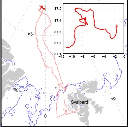
ASCOS contributed to the International Polar Year 2007-2009. The primary objective was to understand the processes leading to the formation and life-cycle of low-level clouds and the role they play in the surface energy budget of the high Arctic during the late summer to early fall transition. ASCOS was interdisciplinary, with science teams focused on meteorology, physical oceanography, atmospheric gas-phase chem-istry, aerosol chemistry and physics, and marine biology. It was the fourth, and largest, in a series of central-Arctic experiments which occurred during 1991 (Leck et al 1996), 1996 (Leck et al 2001) and 2001 (Leck et al 2004; Tjernstr¨om et al 2004). Like its predecessors, ASCOS was conducted onboard the Swedish icebreaker Oden. Oden left Svalbard on 2 August, returning on 9 September 2008. By 12 August, after a few brief open water and marginal ice zone research stations, Oden moored and drifted with a 3 x 6 km ice floe for nearly 21 days. The expedition track, from about N87◦21’ W01◦29’
A detailed description of ASCOS including the instrumentation and measurements is found in Tjernstr¨om et al. (in prep.). Onboard instrumentation used in this study includes a suite of ship-based remote-sensing instruments: a millimeter cloud radar (MMCR; Moran et al 1998), two ceilometer and visibility sensors and a dual wave-length (24/31 GHz) microwave radiometer (MWR) (Westwater et al 2001). The MMCR provides information on the reflectivity of cloud and precipitation particles. Its lowest range gate is at 105 m; clouds and fog below this height are not sensed. The theoretical minimum detectable signal is around -55 dBZ in the lowest few hundred meters, there-fore only very low concentrations of small droplets may not be detected. The MWR provides vertically integrated cloud liquid water path (LWP), employing a statistical bi-linear retrieval resulting in a 25 g m−2 uncertainty (Westwater et al 2001). This uncertainty includes instrument and calibration biases, which at times lead to a drift-ing baseline value. Thus occasional negative LWPs within the uncertainty range are observed. All remote-sensing instruments were operated continuously with very high data recovery. 6-hourly radiosonde profiles were also part of the continually operated onboard measurements.
During the ice drift, a row of masts and instruments were aligned on the ice ex-tending away from the ship to minimize both ship and instrument interference. Two masts, 15 and 30 m, were instrumented for micrometeorological measurements. The 15 m mast supported 5 levels of turbulence measurements from 0.94 to 15.4 m, along with aspirated sensors for profile measurements of mean temperature and humidity. The 30 m mast supported a single sonic anemometer. Sensible heat fluxes are available at all 6 flux-measurement levels, while latent heat fluxes from open-path gas analyzers were at 3.2 and 15.4 m. Turbulent heat fluxes were derived using eddy covariance techniques, with the wind measurements rotated into a consistent streamline-oriented coordinate system using the planar-fit method (Wilczak et al 2001). Data recovery for surface energy budget calculations was quite good, around 80% for sensible and latent heat fluxes. The primary data loss occurred when cold and humid conditions resulted in rime formation on the instruments, primarily during day of year (DoY) 234-236 and 243-245. Turbulent flux uncertainties are difficult to estimate but at least on the order of 10% (Andreas et al 2005). Raw data time series were checked and flagged for data quality prior to flux calculations.
Eight thermocouples measuring surface temperature and four thermocouples mea-suring in-ice temperature were deployed in the vicinity of four broadband radiometers. All themocouples were covered with white heat-shrink wrapping to minimize short-wave heating. Precision Solar Pyranometers (PSP) and Precision Infrared Radiometers (PIR) measuring down- and upwelling shortwave and longwave radiation were installed approximately 1.5 m above an undisturbed snow surface. Initially, two melt ponds were located within approximately 30 m from the radiometers but within the field of view of the instruments. These melt ponds gradually froze over and became covered with snow and rime during the deployment. The radiometers were calibrated against refer-ence radiometers prior to deployment. The factory-specified uncertainty for the PSPs are approximately 3% of incident shortwave radiation for zenith angles encountered during ASCOS, which is equivalent to 3 W m−2 based on median observations. The
2002) revealing a good correspondence throughout the deployment, with an average difference of 0.2±1◦C standard deviation. Also deployed on the ice was a phased-array
sodar system, observing the acoustic backscatter profiles associated with temperature variance up to ∼500 m. Two self-calibrating heat flux plates were buried
approxi-mately 0.05 m below the initial snow surface to measure the near-surface conductive heat flux. The upper faces of the plates were painted white to minimize absorption of shortwave radiation penetrating the upper snow cover. The uncertainty of these in-struments varied as the depth below the snow surface changed with melting, freezing and precipitation, but the absolute RMSE from the mean during the campaign was approximately 0.6 W m−2.
An ocean-observation site contained shortwave radiation sensors above and below approximately 1.8 m thick sea ice, as well as under-ice eddy correlation instruments for measurements of oceanic turbulent fluxes. The shortwave radiation measurements are based on three spectral radiometers spanning wavelengths from 320 to 950 nm with a spectral resolution of 3.3 nm, hence these instruments do not cover the full shortwave spectrum. Two spectral radiometers measure up- and downwelling radiation at the ice surface and one measures radiation transmitted through the sea ice (Nicolaus et al 2010). The under-ice turbulence measurements were obtained using so-called Turbu-lence Instrument Clusters (TICs) which comprise sensors for measuring 3-D velocity, temperature and conductivity (McPhee 2008). TICs were positioned at several levels on a rigid mast which was deployed through the ice and spanned the upper 10 m of the ocean boundary layer. In this study, measurements from the uppermost TIC at 2 m below the ice/ocean interface are used. Current velocities are rotated into a streamline coordinate system and the covariance of vertical deviatory velocity and temperature provide ocean turbulent fluxes (Sirevaag and Fer 2009) The uncertainty in ocean heat flux measurements is on the order of 1 W m−2, however, as with the atmospheric
turbulent fluxes, the variability within a given time period is often larger than the uncertainty.
The majority of on-ice instruments were operational from mid-day on 13 August; all turbulent flux measurements were operational by the 15th. Formation of rime on instruments was a problem primarily during DoYs 234-236 and 243-245. A careful record of the presence of rime and when it was removed was kept by the on-ice science crew. This record has later been used together with other criteria to screen and correct data in post-processing and data quality assurance. All measurement analysis is based on 10-min averaged variables unless noted otherwise.
3 Methods
An energy budget consists of all the components of energy into or out of a system, and the net budget, also referred to as the residual, identifies its respondent sensible and/or latent heating. Conventional energy budget calculations for land surfaces in-herently assume the surface to be an infinitesimally thin layer. This is adequate since all shortwave radiation is typically absorbed within a thin layer near the surface. How-ever, snow and sea ice are semi-transparent to shortwave radiation (Perovich 2005). The definition of the surface energy budget adopted for this study is:
similar to Intrieri et al [2002a]. Qsf cis the residual flux, R represents the net radiative
fluxes, with subscriptss andlcorresponding to short- and longwave, respectively. Hs
and Hl are the turbulent sensible and latent heat fluxes, while C is the conduction of
heat to the snow surface from the ice. Flux signs are defined according to their effect on the surface, positive when heating and negative when cooling, except for the tur-bulent fluxes that are defined traditionally upward such that positive corresponds to a cooling of the surface. In calculating this budget we have assumed that shortwave radiation does not penetrate through the snow, an assumption the authors know to be inaccurate. However, we choose to include this uncertainty rather than making an unsubstantiated guess at the shortwave transmission through the snow layer. Thus, our estimated surface residual will contain a positive, warm bias since we assume net shortwave radiation to be the actual forcing at the surface. Sensitivity tests with rea-sonable assumptions on shortwave radiation penetration (see Perovich 2005) indicated that although this assumption slightly affects the magnitude of the budget residual, it does not greatly alter the residual trends.
The energy budget for the ice, here defined as the entire slab of ice including the snow layer, is defined as:
Qice=Rs−Rsdo+Rl−Hs−Hl+Ho (2)
where Rsdois the downward shortwave radiation transmitted through the ice into the
upper ocean, and Hois the turbulent heat flux from the upper ocean to the ice. Here
the heat conduction near the top of the ice is excluded as it merely acts to redistribute heat. The transmission of shortwave radiation to the ocean is sensitive to snow and ice thickness, neither of which were recorded in detail during the ice drift although ice thickness varied at least between 1.5 and 5 m.
Clouds influence the amount of radiation reaching the surface through scatter-ing, reflecting and absorbing/emission of short- and longwave radiation (e.g. Stephens 1978). Surface cloud radiative forcing (CRF) can be thought of as the effect clouds have on the surface radiation budget.CRFcan be quantified by comparing the surface radiative fluxes under cloudy skies with the radiative fluxes under identical, but clear skies (Schneider 1972; Ramanathan et al 1989):
SW F =Rs(AS)−Rs(CS) (3)
LW F =Rl(AS)−Rl(CS) (4)
CRF=SW F+LW F (5)
whereSWF andLWF are short- and longwave forcing, respectively. Rsand Rlare net
radiative fluxes for all-sky (AS) and clear-sky (CS) conditions. PositiveCRFindicates an enhanced radiative flux warming the surface with the presence of clouds. Note the definition of CRF in Eq. 5 does not include effects on the turbulent heat fluxes at the surface such as in Intrieri et al [2002a]. In this paper, we are only concerned with isolating the instantaneous surfaceCRF component, although we are aware that changes in the radiative forcing will manifest changes in the remaining energy budget components.
unity), well-mixed greenhouse gas concentrations and thermodynamic and ozone pro-files as inputs. No background aerosol profile was used. Thermodynamic propro-files were interpolated to every hour from the radiosondes, resulting in 421 hourlyCRF calcula-tions.
Only 8 cases were identified as clear-sky cases from the vertically-pointing remote sensing suite. Using Eqs. 3 and 4, the mean biases of SWF and LWF during these cases are 13 W m−2 and -4 W m−2, respectively. The LWF bias can be explained by the hemispheric view of the instruments, allowing clouds that were not detected by the fields-of-view of the vertically-pointing remote sensors to alter the observed fluxes. The upward-looking PSP was prone to significant icing for approximately 20% of the hourlyCRF calculations, coinciding with most of the clear-sky cases; the downward-facing PSP remained considerably more ice-free, although not entirely ice-free. There-fore, during times of icing, surface albedo was linearly interpolated in time between radiometer cleanings, and the downward-facing PSP was used to estimate the down-welling shortwave irradiance. Thus, the clear-skySWF is likely biased high since the downward-facing PSP was not perfectly clean, and corrections to downward shortwave will reflect this error. TheSWF bias should be lower during times when icing was not an issue. Thus, since the computed biases of SWF and LWF are believed to be an upper limit, and that instrument icing was not a problem for approximately 80% of the forcing calculations, we estimate the total uncertainty inCRF to be on the order of 10-15 W m−2.
Finally, 5-day back trajectories were calculated from the Global Environmental Research online METEX application to estimate the Lagrangian air-mass trajectories towards Oden. The trajectories are 3-D using the 3-D wind field calculated using reanal-ysis data from the National Centers for Environmental Prediction (Zeng et al 2008). These were computed using Oden’s geographic location during the ice drift, arriving at 200 m above the ship’s location. The 200 m level was chosen as representative of the boundary-layer flow but still away from the surface to avoid trajectory correction when a parcel contacts the underlying surface.
4 Surface and background atmosphere
Surface and near-surface air temperatures experienced substantial variability, while closely following one another during the ice drift (Fig. 2). The mean air temperature generally followed the mean surface temperature minus twice the standard deviation among the multiple sensors, such that the mean air temperature was approximately equal to or colder than the underlying surface, except for a few occasions when the surface was cooler than the air. Therefore, near-neutral to weakly unstable near-surface stratification was commonly observed, in good agreement with the measured sensible heat fluxes. Often the Arctic is associated with strong static stability, however we find a more neutral surface layer during August. Dashed vertical lines indicate approximate transitions between four distinct surface temperature regimes. Temperature maxima during the 1st and 3rd regimes generally remained near the freezing point of fresh (0◦C) and saline water (-1.8◦C; 32 psu), respectively. The 2ndand 4thregimes were
characterized by significant temperature decreases, down to -7◦C during the 2ndregime
and approaching -14◦C on DoY 245. These regimes are chosen based on common
tem-perature trends in chronological order.
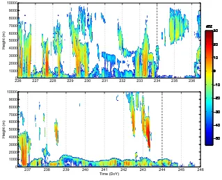
sixth power, are used to identify vertical locations of cloud and precipitation hydrom-eteors (Fig. 3). Multiple cloud layers, some being geometrically thick, precipitating systems, were observed during the first regime from DoY 226 through 233 (Fig. 3, top panel). The temperature drop in the 2ndregime (roughly DoY 234 to 236.5) coincided with weaker reflectivities and tenuous cloud cover that, by the end of DoY 234, tem-porarily dissipated near the surface. Ceilometers confirmed that the low clouds had dissipated by DoY 235, with the only identifiable clouds being the upper-level cirrus from 5000 m up to 9500 m at its deepest. While upper-level clouds were present around the onset (∼DoY 237) and end (∼DoY 243) of the 3rdregime, it was dominated by
a lower stratiform cloud layer (Fig. 3, lower panel). At times, multiple layers were present with ice-crystals falling from a liquid layer near cloud top. The final regime from DoY 244 through 245 initially included the previous low-level stratiform cloud layer, which decreased in depth and reflectivity and became tenuous and altogether absent from the MMCR record early during DoY 245. For approximately six hours around noon on DoY 245, the low cloud layer was again visible in the cloud radar data before disappearing for the remainder of the ice drift. Like the surface temperature division, the cloud scenes observed during each respective regime bear similiarities and warrant these divisions.
Atmospheric parameters such as temperature and water vapor affect the pres-ence and distribution of cloud cover. A comparison of mean temperature and mean water-vapor mixing ratio profiles between the relatively warm 1stand 3rdtemperature regimes suggest that the temperature below 1500 m was between 2-4◦C warmer and
the moisture content was higher by 0.5-1.3 g kg−1during the 1stregime (Fig. 4). Such
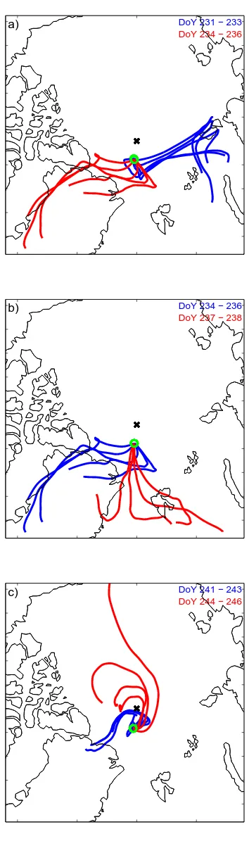
shifts in the thermodynamic structure are likely associated with large-scale air-mass changes. Figure 5 shows 5-day back trajectories arriving 200 m above Oden’s location for up to two days before and two days after the regime transitions. Prior to the onset of the 2ndtemperature regime, the flow was from the Kara Sea (blue in Fig. 5a). Shortly after DoY 233 and near the onset of the 2ndregime, the low-level air trajectories swung around and came from northwest Greenland (red in Fig. 5a and blue in Fig. 5b). By the start of the 3rdregime, the flow arrived from the Fram Strait to the south (red in Fig. 5b). The final, cold temperature regime (DoY 244-245) coincided with an air-mass from the central Arctic basin, and beyond, with long travel times over the Arctic Ocean pack ice (red in Fig. 5c). Clearly, the three regime transitions identified in Fig. 2 are associated with transitions of the low-level air trajectories ending at Oden. Differences in the atmospheric thermodynamics, especially the reduced cloudiness during both the 2ndand 4thregimes, were coincident with these changes in synoptic-scale motions.
5 Energy fluxes
5.1 Turbulent and conductive fluxes
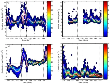
the snow layer. Initially, the conductive flux was negative, directed from the surface into the ice in response to the positive surface forcing. During the cold 2ndregime, heat conduction from the ice turned positive and the snow surface gained heat previously stored within the ice. The peak in positive conductive flux coincides with the absence of low-level cloudiness. During the 3rdregime it remained slightly positive, with larger heat losses occurring again during the 4th regime. The upper ocean heat flux below the ice was most variable during the 1stand 3rdregimes, but on average only slightly larger than 1 W m−2from the ocean into the ice (Fig. 6d).
5.2 Radiative fluxes
The progression of the radiative fluxes are shown in Fig. 7. During the 1st regime, the net shortwave flux was variable and most often ranged between 10-40 W m−2 (Fig. 7a), while the net longwave flux was -10 W m−2to near zero (Fig. 7b). The onset of the first cold regime on DoY 234 coincided with a deficit in net radiation (Fig. 7c). Net shortwave radiation temporarily increased (20-50 W m−2) while net longwave decreased (-40 to -50 W m−2) during DoY 235, consistent with a decrease in the
cloud greenhouse effect at the time when the radar reflectivity suggested diminishing low-level clouds (Fig. 3, top panel). Mean net radiation returned to positive values during the 3rdregime, likely due to the re-emergence of low-level clouds (Fig. 3, lower panel) trapping longwave radiation near the surface. Rapid surface albedo increases were observed during the 2ndregime, due to a combination of snow-fall, freezing melt ponds and rime deposition, while SZA continually increased during the ice drift (Table I). These factors together caused shortwave transmission through the ice to decrease following DoY 236, from approximately 3.5% of the surface downwelling irradiance before, to approximately 1.7% after (Fig. 7d). The radiative fluxes during the cold 4th regime were similar to those of the 2nd regime, coinciding again with tenuous, decreasing cloud radar reflectivity (Fig. 3, lower panel).
6 Cloud radiative forcing
Cloud fraction based on the backscatter intensity of the vertically-pointing cloud ceilometer is shown in Fig. 8 (top panel). Nearly constant overcast skies were ob-served during both of the week-long 1stand 3rdregimes, demonstrating the persistent nature of Arctic cloudiness during August. The lowest cloud base was below 200 m 70% of the time and was rarely observed above 1000 m.
SWF,LWF and totalCRF are shown in the lower panel of Fig. 8. Each of the four regimes are characterized by distinctCRF patterns; the 1st and 3rd regimes exhibit comparable forcing behavior.SWF, ranging from -50 to -25 W m−2, was largest during the 1st regime, after which increased surface albedo and SZA (Table 1) by the start of the 3rdregime caused a decrease inSWF by more than a factor of two relative to the 1st regime. A diurnal cycle inSWF indicates a significant dependence on SZA, with the diurnal amplitude of about 15-22 W m−2at the beginning decreasing to about
10-12 W m−2at the end of the ice drift, similar to values reported by Shupe and Intrieri [2004].
LWF generally ranged between 65-80 W m−2during the 1stregime, and between
70-85 W m−2 during the 3rd regime. Mean
m−2, nearly 5 W m−2 larger and statistically significant than during the 1st regime.
As discussed above, considerable differences in the lower atmospheric thermal structure were observed during these two regimes. As a result of warmer temperatures and higher water vapor content in the lowest few kilometers, longwave clear-sky atmospheric radia-tive emission is enhanced during the 1st regime compare to the 3rd, partially masking the cloud LWF during the 1st regime. This is consistent with the findings of Zhang et al [2001]. TotalCRF reflected this shift in bothSWF andLWF. Clouds warmed the surface by 25-55 W m−2during the 1stregime; this increased to 55-75 W m−2during
the 3rdregime (Fig. 8, black line).
The magnitudes ofSWF andLWF decreased temporarily on DoY’s 234 and 235. ASWF of -25 W m−2at the start of this regime decreased to -10 to -5 W m−2as low-level clouds thinned or disappeared (Fig. 3).LWF simultaneously dropped from∼75
W m−2to nearly 10 W m−2, and together the totalCRFdecreased from∼50 W m−2 to near zero. Similarly, both cloud radiative forcing components decreased during the cold 4thregime. Here,LWF decreased from∼80 to 10 W m−2andSWFfrom -20 W m−2to near zero. Since the meanSWFvaried by, at most, 25 W m−2during both cold regimes,LWF was responsible for the majority of the change in totalCRF, underlining the importance of the cloudLWFat this time of year. Even with uncertainty estimates on the order of 10 to 15 W m−2 as described in 3,CRF estimates indicate a robust cloud-warming effect at the surface during ASCOS.
6.1 Cloud forcing sensitivity
6.1.1 SWF sensitivity
It is important to understand how the critical factors influencingSWFandLWF affect the totalCRF at the surface.SWFdepends on the cloud microphysical properties, the surface albedo and the SZA (Curry et al 1996). Figure 9 shows the influence of SZA, surface albedo and LWP onSWF. The range ofSWFagrees well with the average range reported during SHEBA for similar SZAs (Shupe and Intrieri 2004). The magnitude of shortwave forcing generally increases with decreasing surface albedo, such that a linear fit of the forcing to surface albedo results in an increasedSWFof∼1.8 W m−2for every
which also shows a significant dependence on cloud LWP (Fig. 10b). After having excluded the external parameters of surface albedo and SZA, the remaining variability in the shortwave cloud attentuation is results from variations in cloud geometry, droplet size and phase. Thus cloud structure and composition itself, not only the large SZAs and surface albedo, are also responsible for complex cloud-radiative interactions over the Arctic.
6.1.2 LWF sensitivity
LWF is largely influenced by the cloud’s emissivity dependence on LWP, cloud droplet radius and phase, along with the emission temperature of the cloud. As discussed above, the clear-sky downwelling longwave radiation can further act to modulate the LWF. Figure 11 shows the dependency of LWF on LWP, separated into cloud-base temperature ranges, determined by interpolated radiosonde profiles and ceilometer-determined cloud-base heights. In general, LWF estimates were on the order of 10 W m2 larger during ASCOS than those computed at SHEBA for the similar season and LWP above 50 g m−2(Shupe and Intrieri 2004; Chen et al 2006).LWF increases significantly when LWP increases from near zero to ∼ 50 g m−2, corresponding to an exponential dependence of cloud longwave emissivity on LWP for liquid-containing clouds (e.g. Stephens 1978). Further increases in LWP exert no significant impact on LWF as the cloud radiates as a nearly-ideal black body (Garrett et al 2002; Shupe and Intrieri 2004).LWF from clouds with base temperatures below -10◦C was small
since these clouds typically contained only a limited amount of liquid. The range in LWF for LWP> 50 g m−2 was largest for cloudbase temperatures ranging from -5 to 0◦C. The lower data points forLWF within the cloud-base temperature range
of -5 to 0◦C occurred primarily during the 1st regime when a warmer and moister
atmosphere partly masked enhanced downwelling longwave flux from the cloud. On the other hand, the higherLWF for this temperature range came about during the 3rd regime, characterized by fog or low-level cloud layers with slightly warmer cloud-base temperatures. These low layers were the cause of LWF in excess of 75 W m−2 even when LWP was less than 50 g m−2.
7 Snow and ice energy budgets
Means for the terms in Eqs. 1- 2 across the four regimes are shown both for the snow surface (Fig. 12a) and the sea ice (Fig. 12b), including± 1 standard deviation bars.
low-level mixed-phase clouds prior to DoY 232 could have offset this snow melt. The total residual for the ice and snow system as a whole was 17 W m−2, indicating that the majority of the heat was expended in melting the upper snow layer.
The three subsequent regimes experienced significantly smaller net snow and ice residuals (Fig. 12 and Table 1). Increased losses of heat associated with decreasing cloud cover yielded mean net radiative fluxes that nearly offset each other during the cold regimes. As a result, heat previously stored within the ice was transferred upwards to compensate surface energy loss, resulting in a negative residual for the ice. Thus, the first potential indication of freeze-onset occurred between DoY 234 and 235. However, the surface residual remained slightly positive during the 2nd regime, however we know this surface estimate to be biased warm. The mean residuals during the 3rd regime were small; the variability is larger than the mean value which is not significantly different from zero. An increase in the mean surface albedo from 0.73 to 0.84 occurred during and after the 2ndregime through a combination of freezing melt ponds, rime deposition and new snow fall. By the 4thregime, both mean heat budget residuals were negative due to large deficits in net longwave radiation and a reduction in net shortwave radiation. Turbulent heat fluxes were nearly the same magnitude as both the net radiative and residual fluxes for all but the first regime, implying that the turbulent fluxes act as significant redistributors of the total radiative forcing. Despite variability in the observations, both snow and ice residuals were negative and corresponding temperatures decreased significantly, suggesting that full initiation of the fall freeze-up occurred during the 4thregime, approximately 10 days after the first indication of freeze. We shall return to this temporal difference in the discussion below.
8 Case study
We have demonstrated that the surface energy budget system is largely influenced by the presence, absence and properties of the cloud cover. To illustrate this influence, we investigate DoY 235. A cirrus cloud, sometimes more than 4000 m thick, was overhead during much of this 24-hr period (Fig. 13a). Tenuous low-level clouds were observed by the ceilometer and MMCR in the early morning hours and again after 12 UTC, as an increasingly robust fog deepened into a low-level cloud below 300 m. There was little or no cloud liquid water (Fig. 13e) identifiable until after 12 UTC, coincident with the developing low-level cloud. Analysis of upper-level radiosoundings suggests that colder air was advected over the ice drift during the morning and early afternoon hours, which may have provided the necessary cooling for saturation of liquid water.
Surface temperature varied approximately between -7.5 and -6◦C (Fig. 13b) prior
to 12 UTC, and a linear fit to these first 12 hours suggests no temporal trend. Shortly before 12 UTC surface temperature jumped and continued on an increasing trend through the remainder of the 24-hour period, although the absolute change in temper-ature during the afternoon was only slightly larger than 2◦C. The downwelling radiative
fluxes (Fig. 13c-d) are significantly modified by the cloud scene overhead, and surface responds to these radiative changes. Temperatures below -6◦C were generally
energy residual before 12 UTC were generally larger than -20 W m−2 (median value
-13 W m−2), suggesting that surface radiative forcing resulted in a redistribution of turbulent and conductive heat fluxes which effectively limited the absolute change in surface temperature (Fig. 14c). Temperatures above -6◦C generally occurred as cloud
LWP increased with the deepening lower cloud layer, yielding small but positive net radiation at the surface as a result of a net cloud radiative forcing change of∼30 W
m2. The corresponding change in total surface energy was approximately half of this net radiative forcing change, however the surface temperature increase was limited to only∼2◦C. In-ice temperatures, as well as estimates using an equivalent snow depth,
suggest that a thermal wave in response to the surface forcing penetrated through the snow and into the ice, but only within the uppermost 10 cm below the surface. Given the change in residual forcing of 15 W m−2 and assuming reasonable snow depth, the estimated surface temperature increase should not have been larger than 3◦C, in line
with the observed temperature increase. Although this case is not representative of the entire ASCOS ice drift, it demonstrates how periods of tenuous, or absent, clouds with little liquid water can ”force” the coldest temperature regimes and effectively initiate the system into, or out of, a freeze-up transition for the conditions encountered.
Sensible heat (Fig. 13f) was transferred from the atmosphere towards the surface prior to 09 UTC and then changed sign and remained positive after 10:30 UTC. This is coincident with an increase in cloud LWP from 0 to 10 g m−2 (Fig. 13e), which caused downwelling longwave radiation to increase by ∼20 W m−2 (Fig. 13d). The surface energy balance, forced mainly by the reduction in net longwave deficit due to the developing low cloud, led to a warming of the surface, more quickly than the near-surface air. This caused a destabilization and transitioning from stably stratified to convective conditions. Radiosonde profiles during the day suggest that the modi-fication of the energy at the surface led to a deepening ABL from less than 100 m in the morning to approximately 200 m in the afternoon (Fig. 15, top panel). The sodar backscatter (Fig. 15, lower panel) confirms the shallow boundary-layer depths in the morning; strong acoustic backscatter is an indication of temperature variance associated with turbulence acting in a strong gradient and is commonly observed at the interface between the boundary layer and free troposphere. The increased ABL depth to over 200 m in the afternoon, seen in both temperature and sodar backscatter profiles, coincides with the vertical location of the deepening low-level cloud layer dur-ing the afternoon. Considerdur-ing the negligible changes in the near-surface wind speed over the course of the day (Fig. 13g), these results suggest that neither advection of heat nor increased mechanical mixing directly forced the surface temperature increase on this day. Instead, surface cloud radiative forcing destabilized the lower boundary layer and caused a vertical turbulent transport of sensible heat. However, it can be argued that cold-air advection aloft may have been responsible for the low-level cloud development.
9 Discussion and conclusions
conditions and the cloud liquid water path on the cloud short- and longwave radiative forcing components was determined.
Clear transitions between different regimes are evident in the surface temperature. The radiative fluxes support a division into 4 distinct regimes characterized by differing thermodynamic structure and cloud properties. These regimes are linked to changes in synoptic-scale weather patterns modifying the temperature and humidity profiles and the accompanying cloud field. We have identified a large-scale shift in the atmospheric thermodynamic structure between the 1stand 3rd weeks of the ice drift. Back trajec-tory calculations indicate the flow was from the Greenland and Barent Seas during the 1stweek, bringing warmer and more humid air masses associated with a series of syn-optic fronts. This flow pattern continued early in week 3, but became increasingly more influenced by a high pressure advecting over the central Arctic from Greenland, asso-ciated with a cooler and drier lower troposphere. In response to the varying cloudiness, the radiative fluxes showed the largest variations and dominated the energy budgets. Net shortwave radiation generally ranged between 10-40 W m−2when cloud cover was
present, but could be significantly larger when cloud cover was tenuous or absent, as observed during the two cold regimes. The magnitudes of shortwave effects decreased with time as SZA and surface albedo increased. Net longwave radiation when clouds were present consistently ranged from -10 W m−2to zero, but the deficit was observed to reach as much as -60 W m−2during tenuous cloud periods. The turbulent and con-ductive fluxes were significantly smaller than these, although they were on the same order as the mean net energy fluxes for three of the 4 regimes, making them significant redistributors of the energy imparted by radiative fluxes.
TotalCRF ranged from approximately 25-50 W m−2 during the 1st regime, and
the magnitude increased to 55-75 W m−2during the 3rdregime. The increase in forcing
magnitude was related to variations in bothSWFandLWF components. Mean surface albedo increased from∼0.73 to∼0.84, limiting the shortwave radiation absorption at
the surface, and at the same time the SZA continued to increase, reducing the amount of incident shortwave radiation. The influences of SZA and the surface albedo onSWF, along with the influence of cloud LWP have been examined. The forcing generally increased linearly in combination with increasing LWP and decreasing SZA and surface albedo. SWF exhibited a diurnal cycle of 10-22 W m−2, being largest when SZA and surface albedo were smallest. MeanLWF increased by approximately 5 W m−2 during the ice drift and has been linked to a decrease in the background atmospheric temperature and humidity, which masked a part of the LWF during the 1st regime. However, downwelling longwave radiation did decrease during the 3rd regime relative to the 1stand can be attributed to advection of cooler air in the lower troposphere.
the air, a destabilization of the lower atmosphere occurred and turbulent heat fluxes increased in magnitude, cooling the surface.
Mean energy budget residuals suggest that the initial freeze onset could have begun during the cold 2nd regime, from 21-23 August. Climatological studies using both active and passive satellite measurements and surface temperature observations show a general consensus that interior, central Arctic freeze onset often occurs between the 2nd week of August and early September (Rigor et al 2000; Belchansky et al 2004; Overland et al 2008). Observational studies often use the first instance when a running mean near-surface temperature surpasses the -2◦C threshold to identify the
freeze-up onset. Doing the same for the ASCOS ice drift suggests the freeze onset occurred early on 24 August (DoY 237). This date is similar to that determined with respect to the mean energy budget residual analysis of the sea ice and consistent with previous central Arctic freeze dates reported in the literature (Rigor et al 2000; Nilsson et al 2001; Belchansky et al 2004; Overland et al 2008; Markus et al 2009). The successive progression of the freeze-up during ASCOS was inhibited by low-level stratiform cloud cover during the 3rd regime, causing small but positive energy residuals.
The seasonal freeze-up onset, when temperatures no longer return to the melting point of sea-ice, appears to have happened a week or more after the cold 2nd regime, coinciding with the arrival of drier air with a long residence time in the central Arctic and optically thinner clouds or clear skies. During this 4thtemperature regime, both the mean snow and ice energy budget residuals were negative. Markus et al [2009] have demonstrated that the first indication of freeze, on average, occurs approximately 10 days prior to the time when freeze is observed to persist for the remainder of the season. The 10-day time scale observed may be related to the passage of large-scale weather systems responsible for thermodynamic advection that affects the cloud properties. We have highlighted the processes responsible for this first freeze onset and the transition toward persistent freeze during ASCOS.
The two cold-temperature regimes were associated with tenuous cloud cover, lead-ing to reduced net warmlead-ing by the clouds and subsequent drops in surface temperature. Direct deposition, or riming, of water vapor on the snow surface and ice growth on melt ponds and open leads increased the surface albedo at these times, resulting in a lower net surface shortwave radiation. Heat transfer upwards through the ice and turbulent heat fluxes from the atmosphere to the surface during the final cold regime were insuf-ficient to compensate for the radiative cooling of the surface. Therefore, the clouds, or lack thereof, played a central role for the surface energy budget and the onset of the freeze-up, and we find cloud cover to be a key component in the surface energy budget transitions of the Arctic.
10 Acknowledgements
Norwegian Research Council; Sebastian Gerland is acknowledged for dual-responsibility of data with MN. The Swedish Polar Research Secretariat (SPRS) provided access to the icebreaker Oden and logistical support. Chief Scientists were Caroline Leck and Michael Tjernstr¨om. We are grateful to the SPRS logistical staff and to Oden’s Cap-tain Mattias Peterson and his crew. ASCOS is an IPY project under the AICIA-IPY umbrella and an endorsed SOLAS project.
References
ACIA (2005) Arctic Climate Impact Assesment: Impacts of a warming Arctic. Cam-bridge University Press
Andreas EL, Jordan RE, Makshtas AP (2005) Parameterizing Turbulent Exchange Over Sea Ice: The Ice Station Weddell results. Boundary-Layer Meteorol 114:439– 460
Belchansky GI, Douglas DC, Platonov NG (2004) Duration of the Arctic Sea Ice Melt Season: Regional and Interannual Variability, 1979-2001. J Clim 17:67–80
Birch CE, Brooks IM, Tjernstr¨om M, Milton SF, Earnshaw P, S¨oderberg S, Persson POG (2009) The performance of a global and mesoscale model over the central Arctic Ocean during late summer. J Geophys Res 114, D12104, DOI 10.1029/2008JD010790 Chen Y, Aires F, Francis JA, Miller JR (2006) Observed Relationships between Arctic Longwave Cloud Forcing and Cloud Parameters Using a Neural Network. J Clim 19:4087–4104
Curry JA, Rossow WB, Randall D, Schramm JL (1996) Overview of Arctic cloud and radiation characteristics. J Clim 9:1731–1764
Fu Q, Liou KN (1992) The Correlated k-Distribution Method for Radiative Transfer in Nonhomogeneous Atmospheres. J Atmos Sci 49:2139–2156
Garrett TJ, Radke LF, Hobbs PV (2002) Aerosol Effects on Cloud Emissivity and Surface Longwave Heating in the Arctic. J Atmos Sci 59:769–778
Graversen RG (2006) Do Changes in the Midlatitude Circulation Have Any Impact on the Arctic Surface Air Temperature Trend? J Clim 19:5422–5438
Graversen RG, Wang M (2009) Polar amplification in a coupled climate model with locked albedo. Clim Dyn 33:629–643
Graversen RG, Mauritsen T, Tjernstr¨om M, K¨allen E, Svensson G (2008) Vertical structure of recent Arctic warming. Nature 451:53–57
Intrieri JM, Fairall CW, Shupe MD, Persson POG, Andreas EL, Guest PS, Moritz RE (2002a) An annual cycle of Arctic surface cloud forcing at SHEBA. J Geophys Res 107, C10, DOI 10.1029/2000JC000439
Intrieri JM, Shupe MD, Uttal T, McCarty BJ (2002b) An annual cycle of Arctic cloud characteristics observed by radar and lidar at SHEBA. J Geophys Res 107, C10, DOI 10.1029/2000JC000423
IPCC (2007) Intergovernmental Panel on Climate Change, Forth Assessment Report -The physical science basis. Cambridge University Press
Kay J, L’Ecuyer ET, Gettelman A, Stephens G, O’Dell C (2008) The contribution of cloud and radiation anomalies to the 2007 Arctic sea ice extent minimum. Geophys Res Let 35, L08503, DOI 10.1029/2008GL033451
Leck C, Bigg EK, Covert DS, Heintzenberg J, Maenhaut W, Nilsson ED, Wiedensohler A (1996) Overview of the atmospheric research program during the International Ocean Expedition of 1991 (IAOE-1991) and its scientific results. Tellus 48B:136–155 Leck C, Nilsson ED, Bigg EK, Bcklin L (2001) The atmospheric program of the Arctic Ocean Expedition 1996 (AOE-1996) - an overview of scientific objectives, experi-mental approaches and instruments. J Geophys Res 106,(D23):32,051–32,067 Leck C, Tjernstr¨om M, Matrai P, Swietlicki E, Bigg K (2004) Can Marine
Micro-organisms Influence Melting of the Arctic Pack Ice? EOS 85:25–36
Lindsay RW, Zhang J (2005) The Thinning of Arctic Sea Ice, 1988-2003: Have We Passed a Tipping Point? J Clim 18:4879–4894
Lindsay RW, Zhang J, Schweiger A, Steele M, Stern H (2009) Arctic Sea Ice Retreat in 2007 Follows Thinning Trend. J Clim 22:165–176
Liou KN (1992) Radiation and Cloud Processes in the Atmosphere, Oxford Monographs on Geology and Geophysics No. 20, Oxford University Press, p 487 pp
Liou KN, Fu Q, Ackerman TP (1988) A Simple Formulation of the Delta-Four-Stream Approximation for Radiative Transfer Parameterizations. J Atmos Sci 45:1940–1947 Liu Y, Key JR, Wang X (2008) The influence of changes in cloud cover on recent
surface temperature trends in the Arctic. JClim 21:705–715
Markus T, Stroeve JC, Miller J (2009) Recent changes in Arctic sea ice melt onset, freezeup, and melt season length. J Geophys Res 114, DOI 10.1029/2009JC005436 McPhee MG (2008) Air-Ice-Ocean interaction: Turbulent Boundary Layer Exchange
Processes. Springer
Moran KP, Martnew BE, Post MJ, Kropfli RA, Welsh DC, Widener KB (1998) An unattended cloud-profiling radar for use in climate research. Bull Amer Meteorol Soc 79:443–455
Nicolaus M, Hudson SR, Gerland S, Munderloh K (2010) A modern concept for au-tonomous and continuous measurements of spectral albedo and transmittance of sea ice. Cold Regions Science and Tech 62:14–28
Nilsson ED, Rannik U, Hakansson M (2001) Surface energy budget over the central Arc-tic Ocean during late summer and early freeze-up. J Geophys Res 106 (D23):32,187– 32,205
Overland JE (2009) The case for global warming in the Arctic. In Influence of climate change on the changing Arctic and Sub-Arctic conditions, Springer, pp 13–23 Overland JE, Turner J, Francis J, Gillett N, Marshall G, Tjernstr¨om M (2008) The
Arctic and Antarctic: Two Faces of Climate Change. EOS 89:177–184
Perovich DK (2005) The aggregate-scale portioning of solar radiation in Arctic sea ice during the Surface Heat Budget of the Arctic Ocean (SHEBA) field experiment. J Geophys Res 110, DOI 10.1029/2004JC002512
Perovich DK, Richter-Menge JA, Jones KF, Light B (2008) Sunlight, water, and ice: Extreme Arctic sea ice melt during the summer of 2007. Geophys Res Let 35, L11501, DOI 10.1029/2008GL034007
Persson POG, Fairall CW, Andreas EL, Guest PS, Perovich DK (2002) Measurements near the Atmospheric Surface Flux Group tower at SHEBA: Near-surface conditions and surface energy budget. J Geophys Res 107 (C10), DOI 10.1029/2000JC000705 Polyakov I, Timokhov L, Hansen E, Piechura J, Walczowski W, Ivanov V, Simmons H,
Ramanathan V, Cess RD, Harrison EF, Minnis P, Barkstrom BR, Ahmad E, Hart-man D (1989) Cloud-radiative forcing and climate: Results for the Earth Radiation Budget Experiment. Science 243:57–63
Rigor IG, Colony RL, Martin S (2000) Variations in Surface Air Temperature Obser-vations in the Arctic 1979-97. J Clim 13:896–914
Roebber PJ, Bruening SL, Schultz DM, Cortinas Jr JV (2003) Improving Snowfall Forecasting by Diagnosing Snow Density. Weather and Forecasting 18:264–287 Ruffieux D, Persson POG, Fairall CW, Wolfe DE (1995) Ice pack and lead surface
energy budgets during LEADEX 1992. J Geophys Res 100:4593–4612
Schneider SH (1972) Cloudiness as a global climate feedback mechanism: The effects on the radiation balance and surface temperature variations in cloudiness. J Atmos Sci 29:1413–1422
Serreze MC, Holland MM, Stroeve J (2007) Perspectives on the Arctic’s shrinking sea-ice cover. Science 315:1533–1536, DOI 10.1126/science.1139426
Shimada Kea (2006) Pacific Ocean inflow: Influence on catastrophic reduction of sea ice cover in the Arctic Ocean. Geophys Res Let 33, L08605, DOI 10.1029/2005GL025624 Shupe MD, Intrieri JM (2004) Cloud Radiative Forcing of the Arctic Surface: The Influ-ence of Cloud Properties, Surface Albedo, and Solar Zenith Angle. J Clim 17:616–628 Sirevaag A, Fer I (2009) Early Spring Oceanic Heat Fluxes and Mixing Observed from Drift Stations North of Svalbard. J Phys Oceanogr 39(12):3049–3069, DOI 10.1175/2009jpo4172.1
Stephens GL (1978) Radiation Profiles in Extended Water Clouds. II: Parameterization Schemes. J Atmos Sci 35:2123–2132
Tjernstr¨om M, Leck C, Persson POG, Jensen ML, Oncley SP, Targino A (2004) The summertime Arctic atmosphere: Meteorological measurements during the Arctic Ocean Experiment (AOE-2001). Bull Amer Meteorol Soc 85:1305–1321
Tjernstr¨om M, Zagar M, Svensson G, Cassano JJ, Pfeifer S, Rinke A, Wyser K, Dethloff K, Jones C, Semmler T, Shaw M (2005) Modelling the Arctic Boundary Layer: An Evaluation of Six ARCMIP Regional-Scale Models Using Data from the SHEBA Project. Boundary-Layer Meteorol 117:337–381, DOI 10.1007/s10546-004-7954-z Walsh JE, Chapman WL (1998) Arctic Cloud-Radiation-Temperature Associations in
Observational Data and Atmospheric Reanalyses. J Clim 11:3030–3045
Westwater ER, Han Y, Shupe MD, Matrosov SY (2001) Analysis of integrated cloud liquid and precipitable water vapor retrievals from microwave radiometers during SHEBA. J Geophys Res 106:32,019–32,030
Wilczak JM, Oncley SP, Stage SA (2001) Sonic Anemometer Tilt Correction Algo-rithms. Boundary-Layer Meteorol 99:127–150
Zeng J, Matsunaga T, Mukai H (2008) METEX - A flexible tool for air trajectory calculation. Environmental Modelling and Software 25:607–608
Zhang J, Lindsay R, Steele M, Schweiger A (2008a) What drove the dramatic re-treat of arctic sea ice during summer 2007? Geophys Res Let 35, L11505, DOI 10.1029/2008GL034005
Zhang T, Stamnes K, Bowling SA (2001) Impact of the Atmospheric Thickness on the Atmospheric Downwelling Longwave Radiation and Snowmelt under Clear-Sky Conditions in the Arctic and Subarctic. J Clim 14:920–939
Table 1 Regime classification (DoY-Day of Year), corresponding statistics of surface albedo
αs (including standard deviationσand percentiles), solar zenith angle (SZA) range and the
energy budget flux components for both snow and the ice, all in W m−2. Energy budget
components are defined as in Eqs. 1- 2
Energy budget fluxes for the snow/ice (W m−2)
Time (DoY) Meanαs(σ) Medianαs(25th, 75th) SZA (◦) Rs Rl Hs Hl Hc/ Ho Residual
85
80
0
30
Svalbard
87.1 87.2 87.3 87.4 87.5
−12 −10 −8 −6 −4 −2 0
Fig. 1 Cruise track for ASCOS (light red) and ice drift track (dark red); insert zooms in on
[image:21.612.115.373.42.297.2]226 228 230 232 234 236 238 240 242 244 246
−14
−12
−10
−8
−6
−4
−2
0
Time (DoY)
Temperature (
°
C)
Ts
Mean T s
Mean Ts + 2 std
Mean T
s − 2 std
Tair
Fig. 2 Mean air temperature at approximately 1 m a.g.l. (red) and surface temperatures from
[image:22.612.81.407.33.289.2]226 227 228 229 230 231 232 233 234 235 236 0 1000 2000 3000 4000 5000 6000 7000 8000 9000 10000 Height (m)
237 238 239 240 241 242 243 244 245 246
0 1000 2000 3000 4000 5000 6000 7000 8000 9000 10000 Time (DoY) Height (m) dBZ −50 −40 −30 −20 −10 0 10 20 30 dBZ −50 −40 −30 −20 −10 0 10 20 30 dBZ −50 −40 −30 −20 −10 0 10 20 30 dBZ −50 −40 −30 −20 −10 0 10 20 30 dBZ −50 −40 −30 −20 −10 0 10 20 30 dBZ −50 −40 −30 −20 −10 0 10 20 30 dBZ −50 −40 −30 −20 −10 0 10 20 30 dBZ −50 −40 −30 −20 −10 0 10 20 30 dBZ −50 −40 −30 −20 −10 0 10 20 30 dBZ −50 −40 −30 −20 −10 0 10 20 30 dBZ −50 −40 −30 −20 −10 0 10 20 30
Fig. 3 Radar reflectivity contour time series during the ice drift from the MMCR’s lowest
range gate at 0.105 km up to 10 km. The top panel is the first 10 days, where dashed vertical lines differentiate between the first 2 temperature regimes; the lower panel is a continuation in time from the top panel, showing the 3rd
and 4th
regimes. Reflectivity is sensitive to particle size to the 6th
[image:23.612.91.410.55.314.2]−60 −50 −40 −30 −20 −100 0 10 1000
2000 3000 4000 5000 6000 7000 8000 9000 10000 11000 12000
Temperature (
°
C)
Height a.g.l. (m)
0 1 2 3 4
Water vapor mixing ratio (g / kg)
Mean profile, DoY 228−233 Mean profile, DoY 236−243 Difference
Mean profile, DoY 228−233 Mean profile, DoY 236−243 Difference
Fig. 4 Mean temperature (◦C, left panel) and water vapor mixing ratio (g kg−1, right panel)
for the 1st
regime (DoY 228-233, solid line) and 3rd
[image:24.612.75.416.43.316.2]DoY 231 − 233
DoY 234 − 236 a)
DoY 234 − 236
DoY 237 − 238 b)
DoY 241 − 243
DoY 244 − 246 c)
Fig. 5 5-day back trajectories ending at 200 m above the position of Oden, calculated for
[image:25.612.156.333.43.644.2]Time (DoY)
Sensible heat flux (W m
−2
)
a)
228 230 232 234 236 238 240 242 244 −8 −6 −4 −2 0 2 4 6 8 10 12 5 10 15 20 25 30 35 40 Time (DoY)
Latent heat flux (W m
−2
)
b)
228 230 232 234 236 238 240 242 244 −8 −6 −4 −2 0 2 4 6 8 10 12 5 10 15 20 25 30 35 40 Time (DoY)
Conductive heat flux (W m
−2
)
c)
228 230 232 234 236 238 240 242 244 −10 −8 −6 −4 −2 0 2 4 6 8 10 12 5 10 15 20 25 30 35 40 Time (DoY)
Ocean heat flux (W m
−2
)
d)
228 230 232 234 236 238 240 242 244 −2 0 2 4 6 8 10 12 14 16 18 20 5 10 15 20 25 30 35 40
Fig. 6 Relative frequency distribution time trace for a) sensible, b) latent, c) conductive and
d) oceanic heat flux, all given in W m−2. Colors represent probability of occurrence for a given
[image:26.612.77.437.39.315.2]Time (DoY)
Net shortwave flux (W m
−2
)
a)
228 230 232 234 236 238 240 242 244 0 10 20 30 40 50 60 70 5 10 15 20 25 30 35 40 45 50 Time (DoY)
Net longwave flux (W m
−2
)
b)
228 230 232 234 236 238 240 242 244 −70 −60 −50 −40 −30 −20 −10 0 5 10 15 20 25 30 35 40 45 50 Time (DoY)
Net radiation flux (W m
−2
)
c)
228 230 232 234 236 238 240 242 244 −30 −20 −10 0 10 20 30 40 5 10 15 20 25 30 35 40 45 50 Time (DoY)
Shortwave flux through ice (W m
−2
)
d)
228 230 232 234 236 238 240 242 244 0 2 4 6 8 10 12 14 5 10 15 20 25 30 35 40 45 50
Fig. 7 Same as in Fig. 6 except for a) net shortwave, b) net longwave, c) total net and d)
[image:27.612.77.437.42.317.2]0
0.2
0.4
0.6
0.8
1
Cloud fraction
228
230
232
234
236
238
240
242
244
246
−75
−50
−25
0
25
50
75
100
W / m
2
Time (DoY)
Shortwave forcing
Longwave forcing
Total forcing
Fig. 8 Top panel: 10-minute cloud fraction (0-1) with cloud bases<1000 m (black dots) and
[image:28.612.78.482.36.352.2]0.66 0.70 0.74 0.78 0.82 0.86 0.90
−50
−45
−40
−35
−30
−25
−20
−15
−10
−5
0
Surface albedo
Shortwave forcing (W / m
2
)
o: < 25 g m
−2x: 25−75 g m
−2+: 75−125 g m
−2*: > 125 g m
−273−75
°
75−77
°
77−79
°
79−81
°
81−83
°
83−85
°
Fig. 9 1-hrSWF as a function of surface albedo.SWF data have symbols and shading for
different ranges of cloud LWP (g m−2), shown in the top left corner. Colored lines represent
[image:29.612.79.477.49.432.2]0
0.02 0.04 0.06 0.08 0.1
−50
−45
−40
−35
−30
−25
−20
−15
−10
−5
0
cos(
θ
)
⋅
(1−
α
s
)
Shortwave forcing (W / m
2
)
a
0 50 100 150 200 250
−0.5
−0.4
−0.3
−0.2
−0.1
0
Shortwave attenuation
Liquid water path (g / m
2)
b
[image:30.612.75.481.42.304.2]−25 − 25 g/m2 25 − 75 g/m2 75 − 125 g/m2 > 125 g/m2
Fig. 10 a) 1-hrSWF (W m−2) dependence on the linear relationship between SZA (θ) and
surface albedo (αs) and b) non-dimensional shortwave attenuation as a function of cloud LWP
(g m−2). Shortwave attenuation is the difference between observed and clear-sky downwelling
−25
0
0
25 50 75 100 125 150 175 200 225 250
10
20
30
40
50
60
70
80
90
Liquid water path (g / m
2)
Longwave forcing (W / m
2
)
< −10
°
C
−10
°
C to −5
°
C
−5
°
C to 0
°
C
[image:31.612.96.397.47.340.2]≥
0
°
C
Fig. 11 1-hrLWF (W m−2) as a function of cloud LWP (g m−2), separated by cloud base
temperature ranges from<-10◦C to>0◦C. The solid vertical line represents the zero LWP line; LWP<0 g m−2are included due to the 25 W m−2uncertainty in the measurement. The
−60
−50
−40
−30
−20
−10
0
10
20
30
40
50
60
W / m
2
a) surface energy budget
227−233
234−236.5
237−243
244−245
−60
−50
−40
−30
−20
−10
0
10
20
30
40
50
Time (DoY)
b) ice energy budget
LW RadiationSW Radiation
Sensible heat flux
Latent heat flux Conduction
Net
LW Radiation
SW Radiation Sensible heat flux
Latent heat flux
[image:32.612.77.487.43.458.2]Ocean heat flux Net
Fig. 12 Mean components of the energy budget terms for a) the snow surface and for the b)
sea ice in W m−2, calculated over the four main regimes identified in Section 4. Positive flux
represents a warming and negative flux a cooling, except for sensible and latent heat fluxes, which are defined traditionally where positive is cooling. The snow surface budget includes conduction but excludes ocean heat flux and transmission of shortwave radiation. The ice budget includes ocean heat flux and transmission of solar radiation but excludes conduction. Black variability bars represent±1 standard deviation of the mean fluxes for each respective
Height AGL (m)
Radar reflectivity a
2000 4000 6000 8000
−7.5 −7 −6.5 −6 −5.5 −5
°
C
b
Surface temperature
100 150 200 250
W / m
2 c
Downwelling shortwave
240 260 280 300
W / m
2 d
Downwelling longwave
0 20 40 60
g / m
2 e
Liquid water path
−10 −5 0 5 10 15
W / m
2 f
Sensible heat flux
00:00 03:00 06:00 09:00 12:00 15:00 18:00 21:00 00:003 3.5
4 4.5 5
m / s
Time, DoY 235 g
[image:33.612.80.408.57.486.2]Wind speed
Fig. 13 Time traces of a) MMCR reflectivity (dBZ contours), b) surface temperature (◦C,
black) and linear-fit temperature trends for 12-hour (dashed blue) and 24-hour intervals (dashed red), downwelling c) shortwave and d) longwave radiation (W m−2), e) MWR
re-trieved liquid water path (g m−2), f) sensible heat flux (W m−2) and g) 30 m wind speed (m
s−1) during DoY 235. Note that the cloud radar reflectivity scale is not the same as in Fig. 3;
−60 −40 −20 0 20 40 −8
−7.5 −7 −6.5 −6 −5.5 −5
Surface temperature (
°
C)
W / m2
a
−10 0 10 20 30 40 50 60 70
g / m2
b
−20 −10 0 10
W / m2
c
Net shortwave Net longwave Net radiation
[image:34.612.89.414.47.232.2]Liquid water path Net surface energy
Fig. 14 1-min averaged surface temperature (◦C) as a function of a) net radiative fluxes (W
m−2), b) LWP (g m−2) and c) total surface energy residual (W m−2) during DoY 235. Yellow
2700 272 274 276 278 280 282 284 286 288 290 100
200 300 400 500 600 700 800 900 1000
Equivalent potential temperature (K)
Height a.g.l. (m)
20080822 06UTC 20080822 12UTC 20080822 18UTC 20080823 00UTC
Time, DoY 235
Height a.g.l. (m)
00:000 03:00 06:00 09:00 12:00 15:00 18:00 21:00 00:00
[image:35.612.160.329.41.307.2]50 100 150 200 250 300 350 400 450 500
Fig. 15 Equivalent potential temperature profiles (K, top panel) during 22 August 2008 (DoY