A new frequency domain representation and analysis for subharmonic oscillation

This is a repository copy of A new frequency domain representation and analysis for subharmonic oscillation.

White Rose Research Online URL for this paper: http://eprints.whiterose.ac.uk/74674/

Monograph:

Li, L.M. and Billings, S.A. (2011) A new frequency domain representation and analysis for subharmonic oscillation. Research Report. ACSE Research Report no. 1026 . Automatic Control and Systems Engineering, University of Sheffield

[email protected] https://eprints.whiterose.ac.uk/ Reuse

Unless indicated otherwise, fulltext items are protected by copyright with all rights reserved. The copyright exception in section 29 of the Copyright, Designs and Patents Act 1988 allows the making of a single copy solely for the purpose of non-commercial research or private study within the limits of fair dealing. The publisher or other rights-holder may allow further reproduction and re-use of this version - refer to the White Rose Research Online record for this item. Where records identify the publisher as the copyright holder, users can verify any specific terms of use on the publisher’s website.

Takedown

If you consider content in White Rose Research Online to be in breach of UK law, please notify us by

A New Frequency Domain Representation and

Analysis For Subharmonic Oscillation

L. M. Li and S. A. Billings

Department of Automatic Control

and Systems Engineering,

University of Sheffield, Sheffield

Post Box 600 S1 3JD

UK

Research Report No. 1026

A New Frequency Domain Representation and

Analysis For Subharmonic Oscillation

L. M. Li and S. A. Billings*

Department of Automatic Control and Systems Engineering University of Sheffield

Sheffield S1 3JD UK

*_{[email protected]}

Abstract: For a weakly nonlinear oscillator, the frequency domain Volterra kernels, often called the generalised frequency response functions, can provide accurate analysis of the response in terms of amplitudes and frequencies, in a transparent algebraic way. However a Volterra series representation based analysis will become void for nonlinear oscillators that exhibit subharmonics, and the problem of finding a solution in this situation has been mainly treated by the traditional analytical approximation methods. In this paper a novel method is developed, by extending the frequency domain Volterra representation to the subharmonic situation, to allow the advantages and the benefits associated with the traditional generalised frequency response functions to be applied to severely nonlinear systems that exhibit subharmonic behaviour.

Keywords: Volterra series, GFRFs, subharmonics

1.

Introduction

Nonlinear oscillations are widely found in classical mechanics, electronic, communications, biology, and many other science branches.

In general, closed-form analytical solutions are not available for those nonlinear oscillators described by nonlinear differential equations under external periodic excitation, therefore approximation schemes are often used in qualitative and quantitative investigations. In order to derive the estimated solution of a nonlinear oscillator, in terms of the amplitude A and the frequency , a number of analytical approximation methods has been developed, including the describing function method(Krylov and Bogolyubov, 1947), harmonic balance method(Stoker, 1950),

perturbation methods(Hagedorn, 1988) etc.

However, the Volterra series representation has limitations. Volterra series can generally be used in the analysis of so-called weakly nonlinear systems, which significantly restricts its capacity of application in the representation and analysis of a large number of severely nonlinear phenomena. One of the most common severely nonlinear phenomena are subharmonic oscillations, in which the oscillation frequency is a fraction of that of the external excitation. Analytical approximation methods have been applied in the calculation of subharmonic solutions (Stoker, 1950; Nayfeh and Mook, 1979; Hayashi, 1953;Hassan, 1994) , but these were mainly restricted to specialised nonlinear structures or for a reduced number of harmonics in the solution in order to simplify the associated computations, resulting in a loss of generality and accuracy. In the Volterra series domain, Li and Billings(2005) studied the Volterra representation based on a MISO discrete time parametric modelling approach. However this representation is only valid at the specific excitation amplitude point.

In this paper the frequency domain Volterra representation is generalised for the first time to the subharmonic oscillation case which will be valid over the whole excitation amplitude range. The estimation of the frequency domain ‘kernels’ is discussed and the analysis of the subharmonic oscillations based on the new ‘kernels’ is presented based on two illustrative examples.

2.

Volterra series representation in the time and frequency domain

Volterra series modelling has been widely studied for the representation, analysis and design of nonlinear systems. Consider a nonlinear system defined by the nonlinear mapping

y(t)T[u(t)] (1) where u(t) and y(t) are the excitation input and response respectively. In the framework of weak nonlinearity, (1) can be described by Volterra(1930) series modeling as

 1

) ( )

(

n n

t y t

y (2)

where y_n(t) is the ‘n-th order response’ of the system

   

 

  

  



n

i i i

n n

n n

d t u h

t u t

y

1

1, ) ( )

( )] ( [ ) (

  

 _

 n0 (3)

] [

n

T is called the ‘nth-order Volterra operator’, and h_n(₁, ,_n) is called the ‘ nth-order kernel’ or ‘nth-order impulse response function’. If n=1, this reduces to the familiar linear convolution integral. In this sense, the Volterra model is a direct generalization of the linear convolution integral, therefore providing an intuitive representation in a simple and easy to apply way.

A valid Volterra series representation means valid Generalised Frequency Response Functions(GFRF’s). The GFRF’s are obtained by taking the multi-dimensional Fourier transform of h_n():

n n n n n n

n h j d d

H (1, , )__ __ (1, , )exp( (11  )) 1   (4) The generalized frequency response functions represent an inherent and invariant property of the underlying system, and have been widely used in the analysis and characterization of nonlinear phenomena(Schetzen, 1980).

In the nonlinear oscillation problem, the excitation is in sinusoidal format as

t j t j e A e A t A t

u      

2 2

) cos( )

( (5)

The first order response y1(t) can be derived from (3), in the view of (5), as

(Schetzen, 1980) ] ) ( Re[ ) ( 2 A ) ( 2 A ) ( ) ( ) ( 1 1 1 1 1 t j t j t j e AH e H e H d t u h t y                     (6)

Here ‘Re’ means real part of a complex number. Similarly, the second order response

) ( 2 t

y and the third order response y3(t)can be expressed in terms of the second order

and the third order FRFs as in (7)

] ) , ( Re[ ) 2 ( 2 ] ) , ( Re[ ) 2 ( 2 ) ( ) ( ) , ( ) ( 0 2 2 2 2 2 2 1 2 1 2 1 2 2 t j t j e H A e H A d d t u t u h t y            _{ }             (7)

and in (8), respectively

] ) , , ( Re[ ) 2 ( 6 ] ) , , ( Re[ ) 2 ( 2 ) ( ) ( ) ( ) , , ( ) ( 3 3 3 3 3 3 2 1 3 2 1 3 2 1 3 3 t j t j e H A e H A d d d t u t u t u h t y   _{  }                                (8)

The total response can be obtained by combining (6)—(8) as

              ] ) , , ( Re[ ) 2 ( 6 ] ) , , ( Re[ ) 2 ( 2 ] ) , ( Re[ ) 2 ( 2 ] ) , ( Re[ ) 2 ( 2 ] ) ( Re[ ) ( ) ( ) ( ) ( 3 3 3 3 3 0 2 2 2 2 2 1 3 2 1 t j t j t j t j t j e H A e H A e H A e H A e H A t y t y t y t y              

 (9)

) 1 ( 3 ) 1 ( 3 3 3 3 3 ) 0 ( 2 2 2 2 2 1 1 1 ) , , ( ) , , ( ) , ( ) , ( ) ( jI R H jI R H R H jI R H jI R H                       (10)

the analysis of the response of a nonlinear oscillation in (9), in terms of the fundamental frequency and harmonics, can then be readily obtained using the first 3 orders of GFRFs as

) 3 sin( ) 3 cos( ) 2 sin( ) 2 cos( ) sin( ) cos( . ) ( 3 3 2 2 1 1 t b t a t b t a t b t a c d t y              (11a) where 3 3 3 3 3 3 2 2 2 2 2 2 ) 1 ( 3 3 1 1 ) 1 ( 3 3 1 1 ) 0 ( 2 2 ) 2 ( 2 , ) 2 ( 2 , ) 2 ( 2 , ) 2 ( 2 , ) 2 ( 6 , ) 2 ( 6 , ) 2 ( 2 . I A b R A a I A b R A a I A AI b R A AR a R A c d             (11b)

A typical example showing the advantages using a Volterra series model is the Wiener system. Figure 1 shows the schematic depiction of the Wiener model, which consists of a linear dynamic L followed by a static nonlinearity

3 3 2 2 1 )

(x kx k x k x

N    .

Fig. 1 Wiener model

A nonlinear differential equation model between the excitation u(t)and the response

) (t

y is not directly available. But this type of system can be succinctly represented by a finite order Volterra series model

                                 3 2 1 3 2 1 3 2 1 3 2 1 2 1 2 1 2 1 ) ( ) ( ) ( ) ( ) ( ) ( ) ( ) ( ) ( ) ( ) ( ) ( ) (                   d d d t u t u t u l l l k d d t u t u l l k d t u l k t y (12)

and accurately solved by the algebraic approach using GFRFs in (13), following the procedure in (9)—(11).

Despite the effectiveness and usefulness shown in many nonlinear system analyses, it has been clear that many severely nonlinear phenomena, such as sub/super-harmonics, cannot be represented by the Volterra series. In the next section, an attempt is made in order to extend the computational benefits of the Volterra representation—in the frequency domain—to the approximation of the solution of subharmonic oscillations, generally at higher accuracies.

3.

Subharmonic system representation and estimation in the

frequency domain

3.1Representation of subharmonic oscillation in the frequency domain

Subharmonic oscillation is where the excitation frequency is an integral multiple of the oscillation frequency. Subharmonic oscillations are basically frequency domain phenomena, but the analysis has been mainly carried out in the time domain using for example the bifurcation diagram in the literature. The analytical computation of approximation solutions for subharmonic oscillations has also been reported using the harmonic balance method (Stoker, 1950) and using the Krylov-Bogolybov method(Landa 2001), etc.

Subharmonic systems cannot generally be represented by Volterra series in the time domain due to the Periodic steady state theorem [Boyd et al, 1984] which states that the steady state response of a Volterra series model will have the same period as the periodic input. However, it will be shown below that this restriction in the time domain will not prevent frequency domain Volterra style expression and benefits being generalised to the analysis of subharmonic oscillations in the frequency domain.

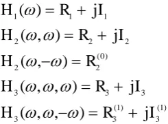
Consider a subharmonic system example. Figure 2 shows a Bifurcation Diagram and the frequency domain counterpart, a response spectrum map (RSM) (Billings and Boaghe, 2001), of the Duffing equation (14).

) cos( )

( )

( ) ( )

( 3

3

1y t k y t A t

k t y c t y

m       (14)

Fig. 2. (a) Bifurcation diagram and (b) response spectrum map for the Duffing

oscillator (14) with m=1, c=0.03, k1=0.8, k =0.15 and 3 3 rad/sec

harmonic components. When A reaches 5.3, there is a sudden behaviour change, with the steady and strong presence of both a 1/3 subharmonic and the fundamental harmonic, together with weaker harmonic components at higher odd multiples. This is a typical weakly nonlinear to severely nonlinear change. When A reaches 7.8, the system is back to weak nonlinearity. The oscillatory solution for the above subharmonic range will have the following form

        ) sin( ) cos( ) sin( ) cos( ) sin( ) cos( ) ( 3 5 3 / 5 3 5 3 / 5 3 / 3 3 / 3 3 1 3 / 1 3 1 3 / 1 t b t a t b t a t b t a t y       (15)

By looking at the link between (9) and (11) in the weak nonlinearity framework, it is both intuitive and reasonable to assume that (15) can have a similar frequency domain expression as in (9), in terms of the auxiliary ‘GFRFs’ H_1/3(), H_3/3()and H_5/3() etc, to give (16).

                 ] ) , , , , ( Re[ ) 2 ( 20 ] ) , , , , ( Re[ ) 2 ( 10 ] ) , , , , ( Re[ ) 2 ( 2 ] ) , , ( Re[ ) 2 ( 6 ] ) , , ( Re[ ) 2 ( 2 ] ) ( Re[ ) 2 ( 2 ) ( ) ( ) ( ) ( 3 1 3 1 3 1 3 5 3 1 3 1 3 1 3 1 3 1 3 1 3 1 3 1 3 1 3 1 3 1 3 / 5 5 3 1 3 1 3 1 3 1 3 1 3 / 5 5 3 1 3 1 3 1 3 1 3 1 3 / 5 5 3 1 3 1 3 1 3 / 3 3 3 1 3 1 3 1 3 / 3 3 3 1 3 / 1 3 / 5 3 / 3 3 / 1 t j t j t j t j t j t j e H A e H A e H A e H A e H A e H A t y t y t y t y                             (16)

It can be seem from (16) that the 3rd order subharmonic 1/3 is made up of contributions from all odd orders of the auxiliary ‘GFRFs’, namely H_1/3(),H_3/3()and

) (

3 / 5 

H etc. Similarly the fundamental frequency has contributions fromH_3/3()andH_5/3()etc, and so on. In this sense the subharmonic system can now have a Volterra-like representation in the frequency domain, making it possible to obtain a solution using algebraic approaches if the auxiliary ‘GFRFs’ are known.

                         ] ) , , , , ( Re[ ) 2 ( 20 ] ) , , , , ( Re[ ) 2 ( 10 ] ) , , , , ( Re[ ) 2 ( 2 ] ) , , , ( Re[ ) 2 ( 12 ] ) , , , ( Re[ ) 2 ( 8 ] ) , , , ( Re[ ) 2 ( 2 ] ) , , ( Re[ ) 2 ( 6 ] ) , , ( Re[ ) 2 ( 2 ] ) , ( Re[ ) 2 ( 2 ] ) , ( Re[ ) 2 ( 2 ] ) ( Re[ ) 2 ( 2 ) ( ) ( 1 1 3 1 5 1 1 2 1 4 1 1 1 3 1 1 2 1 1 1 1 1 1 1 1 / 5 5 1 1 1 1 1 / 5 5 1 1 1 1 1 / 5 5 0 1 1 1 1 / 4 4 1 1 1 1 / 4 4 1 1 1 1 / 4 4 1 1 1 / 3 3 1 1 1 / 3 3 0 1 1 / 2 2 1 1 / 2 2 1 / 1 1 / t j n n n n n n t j n n n n n n t j n n n n n n t j n n n n n t j n n n n n t j n n n n n t j n n n n t j n n n n t j n n n t j n n n t j n n k k n

n n n n n n n n n n n n n n n n n n n n e H A e H A e H A e H A e H A e H A e H A e H A e H A e H A e H A t y t y                                                  (17)

(17) can be seen as a generalisation of the traditional frequency domain Volterra representation into the subharmonic situation. Unlike the traditional frequency domain Volterra kernels, the GFRFs, which can be obtained from parametric differential and difference models, the auxiliary ‘GFRFs’ in (17) will be determined by experimental excitation-response data, which will be explained in detail in subsection 3.2.

3.2Estimation of the auxiliary ‘GFRFs’ for subharmonic oscillation

There has been a number of methods proposed to estimate the GFRFs using non-parametric method(Nam and Powers, 1994;Cho and Powers, 1994;Boyd et al, 1983). But these methods can not be used in the estimation of the auxiliary ‘GFRFs’ in (17), in the subharmonic situation. For example, the FFT based method(Powers and Nam, 1994) is derived based on a time domain Volterra representation, which does not exist for subharmonic systems. Recently Li and Billings(2011) proposed a new method of estimating the GFRFs using time domain data, which can be extended to address the problem of estimation of the auxiliary ‘GFRFs’ in the presence of subharmonic oscillations.

It is assumed that the subharmonics occur over the excitation amplitude range

) ,

(AL AU

A . Then (17) can be re-expressed as

                l n l n l n l n l n n n n n n n n n n n n n n n n n n n n t b t a c d t b t a t b t a t b t a t b t a t b t a c d t y )] sin( ) cos( [ . ) sin( ) cos( ) sin( ) cos( ) sin( ) cos( ) sin( ) cos( ) sin( ) cos( . ) ( / / 5 / 5 5 / 5 4 / 4 4 / 4 3 / 3 3 / 3 2 / 2 2 / 2 1 / 1 1 / 1            

 (18)

even as even and odd, as odd , 2 , 1 , . ) ( ) ( / / ) ( ) ( / / , 4 , 2 ) 0 ( / l k l k N l I A b R A a R A c d N l k k l n k n l N l k k l n k n l

k k n

n k n k n k              (19)

using the definitions

) 1 ( / 5 ) 1 ( / 5 ) 1 ( / 5 1 1 1 1 1 / 5 5 ) 3 ( / 5 ) 3 ( / 5 ) 3 ( / 5 1 1 1 1 1 / 5 5 ) 5 ( / 5 ) 5 ( / 5 ) 5 ( / 5 1 1 1 1 1 / 5 5 ) 0 ( / 4 ) 0 ( / 4 1 1 1 1 / 4 4 ) 2 ( / 4 ) 2 ( / 4 ) 2 ( / 4 1 1 1 1 / 4 4 ) 4 ( / 4 ) 4 ( / 4 ) 4 ( / 4 1 1 1 1 / 4 4 ) 1 ( / 3 ) 1 ( / 3 ) 1 ( / 3 1 1 1 / 3 3 ) 3 ( / 3 1 ) 3 ( / 3 ) 3 ( / 3 1 1 1 / 3 3 ) 0 ( / 2 ) 0 ( / 2 1 1 / 2 2 ) 2 ( / 2 ) 2 ( / 2 ) 2 ( / 2 1 1 / 2 2 ) 1 ( / 1 ) 1 ( / 1 ) 1 ( / 1 1 / 1 ) , , , , ( ) 2 1 ( 20 ) , , , , ( ) 2 1 ( 10 ) , , , , ( ) 2 1 ( 2 ) , , , ( ) 2 1 ( 12 ) , , , ( ) 2 1 ( 8 ) , , , ( ) 2 1 ( 2 ) , , ( ) 2 1 ( 6 ) , , ( ) 2 1 ( 2 , ) , ( ) 2 1 ( 2 ) , ( ) 2 1 ( 2 , ) ( ) 2 1 ( 2 n n n n n n n n n n n n n n n n n n n n n n n n n n n n n n n n n n n n n n n n n n n n n n n n n n n n n n n n n n n n n n n n n n n n n n n n n n n n n n n n jI R H H jI R H H jI R H H R H H jI R H H jI R H H jI R H H jI R H H R H H jI R H H jI R H H                                                                              (20)

From (19), the odd multiples of the lowest subharmonics will be generated by odd order ‘GFRFs’, and even multiples of lowest subharmonics will be generated by even order ‘GFRFs’.

The whole procedure of estimating the auxiliary ‘GFRFs’ will consist of two steps. First, select M excitation amplitude points

M i

A_i, 1,2,

At each excitation amplitude, the excitation-response data are collected and used to estimate the d.c term and the coefficients a_k/n and b_k/n for each non-negligible frequency at different excitation amplitudes using a Least Square(LS) procedure based on (18). The results are M pairs of estimates of a bi i M

n l i

n

l and ˆ , 1,2,

ˆ []

/ ] [

/  with

M> N/2+ 1—here N is the order of the auxiliary ‘GFRFs’ that need to be determined.

Next, by assuming that the auxiliary ‘GFRFs’ in (19) remain invariant over the whole excitation amplitude range A(AL,AU)where the subharmonic exists, then feed the



  

 

  

 

    

  

 

  

 

  

k

l n k l n k n k i i

n l

i n l

I R

A

b a

) (

/ ) (

/ /

] [

/ ] [

/

ˆ ˆ

(21)

Standard Least Square can then be applied to (21) to obtain () / ˆ l n k

R and Iˆ_k(l_/)_n.

The accuracy of the estimation depends on two factors, the number of the harmonic frequencies l and the order of auxiliary ‘GFRFs’ N, chosen from (18) and (19) respectively.

4.

Illustrative examples

Two examples will be shown in this section to demonstrate the effectiveness of the proposed method. The first example is the analysis of 1/2 subharmonic oscillation for a quadratic system, and the second example is the analysis of a 1/3 subharmonic oscillation for a Duffing oscillator which has been extensively studied before using traditional analytic approximation methods, whose results will be compared with the new method.

4.1 Quadratic nonlinear oscillation

Consider a nonlinear oscillator with quadratic nonlinearity

) cos( )

( )

( ) ( )

( 2

2

1yt k y t A t

k t y c t

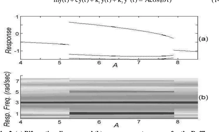
y       (22) with c= 0.2, k1= 1,k3= 0.1. Eqn (22) will have a 1/2 subharmonic at  =2, which is clearly shown in the RSM in Figure 3b. Combined with the response curve in Figure 3a it can be found that initially a relatively weak 1/2 subharmonic appears at

) 6 . 6 , 2 . 6 (



A , followed by a strong 1/2 subharmonic appearance at A(6.6,12.2). When the excitation amplitude is greater than 12.2, the system becomes unstable. The current study will focus on the A(6.6,12.2)section with the 1/2 subharmonic.

Fig 3. (a) Response amplitude (b) the RSM: for system (19) at =2

M i

b

a i

n l i

n

l andˆ , 1,2,

ˆ []

/ ] [

/  along the excitation amplitude were obtained from (18) using a LS routine, each LS estimation involving 1000 excitation-response data. The

amplitude of the estimated 1/2 subharmonic, that is, ˆ ˆ[], 12 28

2 / 1 ] [

2 /

1 b i , , ,

ai i





 , is

shown in Figure 4(solid line). These estimates [] / ] [

/ and ˆ

ˆ i

n l i

n

l b

a were fed into (21) to obtain the amplitude invariant auxiliary 9thorder ‘GFRFs’ using another LS routine. The LS result of Rˆ_k(l_/)₂ jIˆ_k(l_/)₂for the 1/2 subharmonic amplitude case is plotted in Figure 4(dashed line), which indicates that the order of the auxiliary ‘GFRFs’ is sufficient for frequency domain representation in terms of the accuracy. This is also the case for other harmonics as well. The complete results for the auxiliary ‘GFRFs’, which are invariant over the whole excitation amplitude section A(6.6,12.2), are listed in Table 1.

Fig. 4. The amplitude of ½ subharmonic component obtained by LS estimate in left

side of (21), i.e, aˆ₁[_/i]₂bˆ₁[_/i₂] (solid) and by the estimated auxiliary ‘GFRF’ in the

right side of (21), i.e., 

k k

k i H A (1)

2 / 2 /

(Dashed).

) 1 (

2 / 1 ˆ

H -13.2433 +18.5018j (0) 2 / 6 ˆ

H 0.0200

) 0 (

2 / 2 ˆ

H 0.7169 (2)

2 / 6 ˆ

H 0.0001 + 0.0062j

) 2 (

2 / 2 ˆ

H -0.3190 + 0.1472j (1) 2 / 7 ˆ

H 0.0577 - 0.0672j

) 1 (

2 / 3 ˆ

H 5.6862 - 7.3720j (3) 2 / 7 ˆ

H 6.5682e-04- 6.1868e-04j

) 3 (

2 / 3 ˆ

H 0.0183 - 0.0216j (0) 2 / 8 ˆ

H -6.0694e-04

) 0 (

2 / 4 ˆ

H -0.2242 (2)

2 / 8 ˆ

H 6.4537e-06- 1.9921e-04j )

2 (

2 / 4 ˆ

H -0.0008 - 0.0625j (1) 2 / 9 ˆ

H -0.0014 + 0.0016j

) 1 (

2 / 5 ˆ

H -0.8654 + 1.0519j (3) 2 / 9 ˆ

H -2.1165e-05+ 1.8585e-05j

) 3 (

2 / 5 ˆ

H -0.0065 + 0.0068j

Table 1. The auxiliary ‘GFRFs’ estimated for the subharmonic system (22) over

) 2 . 12 , 6 . 6 (



Arbitrarily selecting an excitation amplitude point A=7.83, which was not used in the above estimation procedure, and computing the solution using the auxiliary ‘GFRFs’ in Table 1 gives

) sin( 0627 . 0 ) cos( 0624 . 0 ) sin( 4355 . 0 ) cos( 4940 . 2 ) sin( 4978 . 2 ) cos( 5127 . 1 8058 . 0 ] ) Re[( ] ) Re[( ] ) Re[( ] ) Re[( ) ( ) ( 2 3 2 3 2 1 2 1 9 , 7 , 5 , 3 ) 3 ( 2 / 8 , 6 , 4 , 2 ) 0 ( 2 / 8 , 6 , 4 , 2 ) 2 ( 2 / 9 , 7 , 5 , 3 , 1 ) 1 ( 2 / 3

1 /2 7.8 3 2 3 2 2 2 2 2 2 1 2 t t t t t t e H A H A e H A e H A t y t y t j k k k k t j k k t j k k k k A k k k k                                  (23)

Solution (23) is irrespective of the sampling interval.

In Figure 5, the algebraic solution as in (23) is compared with the numerical solution from (22), showing a perfect overlap. This suggests that the auxiliary ‘GFRFs’ in Table 1 serve as invariant ‘kernels’, like the traditional GFRFs for weakly nonlinear system, over the whole excitation range A(6.6,12.2), therefore they can be used in the accurate analysis of the subharmonic oscillation over the excitation range concerned.

Fig. 5. Comparison of the numerical solution from (22) (Solid) and the algebraic solution in (23) (Circle)

The amplitude of individual harmonic oscillation components can be described as in (24) which are shown in Figure 6. It can be seen from Figure 6 that the 1/2 subharmonic has a strong presence throughout the whole excitation range, much stronger than that of the fundamental frequency in most of the range except in the beginning and end. It also show that the 3/2 super-subharmonic is relatively weak compared with the dominant 1/2 subharmonic and the fundamental frequency.

Fig. 6. The amplitude of each harmonic components in the response: _{RA_2}1

--Solid, RA_--Dashed, 2

3

_

RA -- Circle

4.2 Cubic nonlinear oscillation

The second example is the symmetric Duffing oscillator which takes the form in (14), with very simple structure but exhibits extremely rich nonlinear phenomena including subharmonics, which has been studied extensively in the past decades. The results using the new method in this paper can therefore be compared with those by the traditional analytic approximation based methods.

In the mechanical framework of (14), m is the mass, c is the damping, k1 is proportional to the stiffness of the spring, and k3is the cubic stiffness.

The RSM for (22) is given in Figure 2b, for m=1, c=0.03, k₁=0.8, k₃=0.15 and

sec / 3 rad



 as in (14). The RSM was obtained using an FFT routine, which shows a 1/3 subharmonic, together with its odd multiples. Because there are no even multiples of 1/3 subharmonic therefore the d.c. term is zero. Qualitatively in the RSM the third order multiple, that is, the 53component is weak, but there is no specific measurement of the weakness. For quantitative analysis, a useful measurement provided by the OLS procedure(Billings, et al., 1988; Wei and Billings, 2004) called Error-Reduction-Ratio(ERR), which indicates, in terms of energy, the contribution of each regressor in the LS estimation, can be adopted here. In our case the ERR gives the percentage contribution of each harmonic in the LS estimation in (18), plotted in Figure 7.

Fig. 7. The energy contribution of each harmonic components in the response: 3

1

--Solid, --Dashed, 3

Figure 7 suggests a predominant 1/3 subharmonic at the beginning with decreasing strength as the amplitude increases, in contrast to that of the fundamental harmonic. At all amplitude points, the contribution from 5/3 harmonic is negligibly small; therefore the response can be sufficiently described by the lowest two harmonics, namely 1/3 subharmonic and 3/3 fundamental harmonic.

) 1 (

3 / 1 ˆ

H -1.0960 - 0.3785j (1) 3 / 3 ˆ

H 1.3709 + 0.1545j

) 3 (

3 / 3 ˆ

H -0.1317 - 0.0039j (1) 3 / 5 ˆ

H -0.2523 - 0.0177j )

3 (

3 / 5 ˆ

H 0.0016 + 0.0006j

Table 2. Auxiliary ‘GFRFs’ for subharmonic system (14)

The next step is the estimation of the auxiliary ‘GFRFs’ sufficient for producing accurate harmonics over the whole subharmonic amplitude range. Up to 5th order GFRFs are adopted in the LS procedure in (21) using 13 estimates from the previous step, with the estimates listed in Table 2.

The solution calculated using the auxiliary ‘GFRFs’ in Table 2 at an arbitrarily select excitation amplitude point A=6.48 is given in (25) and compared with the numerical solution in Figure 8, which again shows a perfect agreement.

) sin( 0.0115 )

cos( 0.8181 )

sin( 0.1033 )

cos( 1.1581

] ) Re[(

] ) Re[(

) ( )

(

3 1 3

1

5 , 3

) 3 (

3 / 5

, 3 , 1

) 1 (

3 / 3 , 1 /3 48

. 6

3 3 2

3 1 2

t t

t t

e H A e

H A

t y t

y

t j

k k

t j

k k

k k A

k k

 

 

 

 

 

 

 

 

 

 

(25)

Fig. 8. . Comparison of the numerical solution for (14) (Solid) and the algebraic solution using GFRFs in Table 2. (Circle)

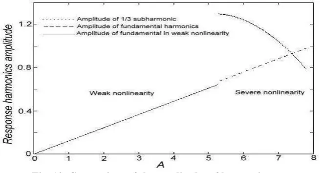
In fact the auxiliary ‘GFRFs’ in Table 2 can give a very accurate solution at any amplitude value within (5.3, 7.8). Stoker (1950, p109) provided an approximation of the 1/3 subharmonic solution for the damped Duffing oscillator (14), which includes the lowest two harmonics, based on the harmonic balance method, as

]

32 8

[

9 ₂

1 2

3 / 1 1 2

3 / 1 3 4 2 7 1 2

k H A k A A k

k   



 (26)

where the excitation u is given by uHcos(t)Gsin(t)with 2 2

G H

A  ,

while the 1/3 subharmonic oscillation has a phase 0, that is, ( ) cos(3 )

1 3 / 1 3

/

1 t A t

The comparison of 1/3 subharmonic oscillation amplitude between the algebraic method using the auxiliary ‘GFRFs’ and the Stoker’s using (26) is given in Figure 9, which shows very accurate estimates by the auxiliary ‘GFRFs’ along the whole amplitude range. This means that the behaviour of the subharmonic oscillation over this amplitude range can be fully characterised by the five auxiliary ‘GFRFs’ in Table 2. Figure 9 also shows that initially the 1/3 subharmonic amplitudes obtained from (26) are close to the true values, but quickly move away. When A is greater than 6.74, equation (26) will no longer give a valid real solution, leaving an unfinished curve. This suggests that even in the current example where the response can be sufficiently described by the first two lowest harmonics on which the harmonic balance solution (26) is based, its accuracy is still not very satisfactory and reliable, and therefore it can only be used in many real situations as a qualitative measure.

Fig. 9. Comparison of the 1/3 subharmonic estimates

It is interesting to see the behaviour of the harmonics in and out of the subharmonic region. When A<5.3, the oscillator (14) has a predominant fundamental harmonic oscillation  , as can be seen from Figure 2, with hardly any superharmonics such as

 ,5

3 etc. During this very ‘weak’ nonlinear region, the response can be almost fully characterised by the first order frequency response function with the amplitude proportional to

12194 . 0 0.0013j

-0.12193

-) (

1 )

(

1 2

3

1   _{j  jc k}  

H

 

 _ (27)

When 5.3<A<7.8, the fundamental harmonic will be governed by (3) 3 / 3 ˆ

H and (3) 3 / 5 ˆ H .

Considering from Table 2 that the (3) 3 / 5 ˆ

H is very small compared with (3) 3 / 3 ˆ

H , the

fundamental harmonic for 5.3<A<7.8 almost fully relates to (3) 3 / 3 ˆ

H with the amplitude proportional to

13180 . 0 0.0039j

-0.1317

-ˆ(3) 3 /

3  

H (28)

function in the weak nonlinear region, as if the linear frequency response function is in operation as usual. This effect is shown in Figure 10, indicating that the severe dynamic change is mainly due to the introduction of 1/3 subharmonic oscillation, which predominates over most of the amplitude range, but in a gain compression manner, that is, its amplitude decreases as the amplitude of the excitation increases. The mechanism behind this abrupt bring-in of additional subharmonic oscillation on top of the normal fundamental harmonic remain largely unexplained and needs further investigation.

Fig. 10. Comparison of the amplitudes of harmonics

5.

Conclusions

Volterra series analysis had been widely applied in the representation, analysis and control of nonlinear systems, and has also been used as an important alternative to the analytical approximation methods in the approximation of solutions of nonlinear oscillations using the Volterra frequency domain computational advantage. However, this advantage has until now been limited to weakly nonlinear oscillations.

The new approach presented in this paper is a generalisation of the frequency domain Volterra kernels to the representation and analysis of a class of severe nonlinear phenomena called subharmonics, which generally could not be studied using traditional Volterra analysis. By introducing a set of sampling independent and amplitude invariant ‘kernels’ in the frequency domain, the solution and analysis of subharmonic oscillations containing any number of harmonics can be efficiently performed in an algebraic way within the required accuracy. To some extent, new frequency representations can be regarded as a sort of inherent frequency domain ‘kernels’ analogous to the classical GFRFs for weakly nonlinear systems. This kind of representation can also be easily modified to accommodate other types of severe nonlinearities such as superharmonics. The new approach has therefore extended the GFRFs based algebraic method to the solution of a much larger family of nonlinear oscillations.

Acknowledgment: LML and SAB gratefully acknowledge that this research was supported by an Advanced Investigator Grant of the European Research Council.

Reference:

Billings, S.A. and Boaghe, O.M., 2001, The response spectrum map, a frequency domain equivalent to the bifurcation diagram, Int. J. of Bifurcation and Chaos, Vol.11, No.7, pp.1961-1975.

Billings, S. A., Korenberg, M.J. and Chen, S., 1988, Identification of non-linear output-affine systems using an orthogonal least-squares algorithm, Int. J. Systems Science, 19 pp.1559-1568.

Billings, S. A. and Peyton Jones, J.C., 1990, Mapping non-linear integro-differential equations into the frequency domain, Int. J. Control, 52 pp. 863-879.

Billings, S. A. and Tsang, K. M., 1989, Spectral analysis for nonlinear systems, Part II— interpretation of nonlinear frequency response functions, Mech Systems and Signal Processing, 3, pp. 341-359.

Boyd, S.P., Chua, L.O. and Desoer, C.A., 1984, Analytical Foundations of Volterra Series, IMA J. of Mathematical Control & Information, Vol. 1, pp.243-282.

Boyd, S., Tang, Y. S. and Chua, L. O., 1983, Measuring Volterra Kernels, IEEE Transactions On Circuits And Systems, vol. cas-30, no. 8, pp.571-577.

Cho, Y. S. and Powers, E. J., 1994, Quadratic system identification using higher order spectra of i.i.d signals, IEEE Transactions on signal processing, vol 42, no. 5, pp.1268-1271.

Chua, L. O. and Tang, Y. S., 1982, Nonlinear oscillation via Volterra series, IEEE Trans. Circuits Syst., vol. 29, pp. 150-168.

Fliess, M., Lamnabhi, M. and Lamnabhi-Lagarrigue, F., 1983, An algebraic approach to nonlinear functional expansions. IEEE Trans Circuits Syst 30:554-570.

Hagedorn, P., Nonlinear Oscillations, Clarendon Press, Oxford, 1988.

Krylov, N. and Bogolyubov, N., 1947, Introduction to Nonlinear Mechanics, Princeton University Press.

Landa, P.S., Regular and Chaotic Oscillations, Springer, New York, 2001.

Li, L.M. and Billings, S.A., 2005, Discrete Time subharmonic modelling and Analysis, Int J of Control 78 No. 16, pp. 1265-1284.

Li, L.M. and Billings, S.A., 2011, Estimation of Generalised Frequency Response Functions for Quadratically and Cubically Nonlinear Systems, Journal of Sound and Vibrations 330 (3) (2011) 461–470.

Ludeke, C., 1951, Predominantly subharmonic oscillations, J.Appl. Phys., 22, pp.1321-1326.

Nam, S. W. and Powers, E. J., 1994, Application of higher-order spectral analysis to cubicallynonlinear system identification, IEEE Trans. Signal Processing, vol. 42, no. 7, pp. 1746-1765.

Nayfeh, A.H. and Mook, D.T., 1979, Nonlinear oscillations, John Wiley & Sons, New York,.

Schetzen, M., 1980, The Volterra and Wiener Theories of Non-linear System, New York, Wiley.

Stoker, J.J., 1950, Nonlinear vibrations in Mechanical and Electrical Systems, Interscience Publishers Inc, New York.

Volterra, V., 1930, Theory of Functionals, Blackie and Sons.

Wei, H. L. and Billings, S.A., 2004, Term and variable selection for nonlinear system identification, Int. J. Control, Vol. 77 (1), pp.86-110.