Characterization of spiraling patterns in spatial rock-paper-scissors games

rock-paper-scissors games

.

White Rose Research Online URL for this paper:

http://eprints.whiterose.ac.uk/84733/

Version: Published Version

Article:

Szczesny, B, Mobilia, M and Rucklidge, AM (2014) Characterization of spiraling patterns in

spatial rock-paper-scissors games. Physical Review E: Statistical, Nonlinear, and Soft

Matter Physics, 90 (3). 032704. ISSN 1539-3755

https://doi.org/10.1103/PhysRevE.90.032704

[email protected] https://eprints.whiterose.ac.uk/ Reuse

Unless indicated otherwise, fulltext items are protected by copyright with all rights reserved. The copyright exception in section 29 of the Copyright, Designs and Patents Act 1988 allows the making of a single copy solely for the purpose of non-commercial research or private study within the limits of fair dealing. The publisher or other rights-holder may allow further reproduction and re-use of this version - refer to the White Rose Research Online record for this item. Where records identify the publisher as the copyright holder, users can verify any specific terms of use on the publisher’s website.

Takedown

If you consider content in White Rose Research Online to be in breach of UK law, please notify us by

Characterization of spiraling patterns in spatial rock-paper-scissors games

Bartosz Szczesny,*Mauro Mobilia,†_{and Alastair M. Rucklidge}‡

Department of Applied Mathematics, School of Mathematics, University of Leeds, Leeds LS2 9JT, United Kingdom

(Received 30 June 2014; published 8 September 2014)

The spatiotemporal arrangement of interacting populations often influences the maintenance of species diversity and is a subject of intense research. Here, we study the spatiotemporal patterns arising from the cyclic competition between three species in two dimensions. Inspired by recent experiments, we consider a generic metapopulation model comprising “rock-paper-scissors” interactions via dominance removal and replacement, reproduction, mutations, pair exchange, and hopping of individuals. By combining analytical and numerical methods, we obtain the model’s phase diagram near its Hopf bifurcation and quantitatively characterize the properties of the spiraling patterns arising in each phase. The phases characterizing the cyclic competition away from the Hopf bifurcation (at low mutation rate) are also investigated. Our analytical approach relies on the careful analysis of the properties of the complex Ginzburg-Landau equation derived through a controlled (perturbative) multiscale expansion around the model’s Hopf bifurcation. Our results allow us to clarify when spatial “rock-paper-scissors” competition leads to stable spiral waves and under which circumstances they are influenced by nonlinear mobility.

DOI:10.1103/PhysRevE.90.032704 PACS number(s): 87.23.Cc,05.45.−a,02.50.Ey,87.23.Kg

I. INTRODUCTION

Ecosystems consist of a large number of interacting organisms and species organized in rich and complex evolving structures [1,2]. The understanding of what helps maintain biodiversity is of paramount importance for the characteriza-tion of ecological and biological systems. It is well established, notably in biology and ecology, that the dynamics of structured populations, where the interactions are limited to some neigh-borhood, generally differs considerably from their spatial-homogeneous counterparts. In this context, local interactions and the spatial arrangement of individuals have been found to be closely related to the stability and coexistence of species and is therefore a subject of continuous research, see, e.g., Refs. [1–3]. Particular attention has been dedicated to cyclic dominance, which was shown to be a motif facilitating the coexistence of diverse species in a number of ecosystems ranging from side-blotched lizards [4,5] and communities of bacteria [6–8] to plants systems and coral reef inver-tebrates [9,10]. It is noteworthy that cyclic dominance is not restricted only to biological systems but also has been found in models of behavioral science [11], e.g., in some public goods games [12]. Remarkably, experiments on three strains ofEscherichia colibacteria in cyclic competition on two-dimensional plates yield spatial arrangements that were shown to sustain the long-term coexistence of the species [6]. Cyclic competitions of this type have been modeled with rock-paper-scissors (RPS) games, where “rock crushes scissors, scissors cut paper, and paper wraps rock” [13].

While nonspatial RPS-like games usually drive all species but one to extinction in finite time [14], their spatial counter-parts are generally characterized by intriguing complex spa-tiotemporal patterns sustaining the species coexistence, see, e.g., Refs. [15–21]. In recent years, many models for the RPS cyclic competition have been considered. In particular, various

*_{[email protected]} †_{[email protected]} ‡_{[email protected]}

two-dimensional versions of the model introduced by May and Leonard [22] have been studied [15,17–19,21,23]. In spatial variants of the May-Leonard model, it was found that mobility implemented by pair-exchange among neighbors can signif-icantly influence species diversity: Below a certain mobility threshold species coexist over long periods of time and self-organize by forming fascinating spiraling patterns, whereas biodiversity is lost when that threshold is exceeded [15]. Other popular RPS models are those characterized by a conservation law at mean-field level (“zero-sum” games). In two spatial dimensions, these zero-sum models are also characterized by a long-lasting coexistence of the species, but in this case the population does not form spiraling patterns [16]. Yet oscillatory behavior has been found in some spatial settings for variants of these zero-sum models [24,25]. On the other hand, while microbial communities in cyclic competition were found to self-organize in a complex manner, it is not clear whether there is a parameter regime in which their spatial arrangement would form spirals as those observed in myxobacteria and in Dictyosteliummounds [26]. In this context, we believe that this work contributes to understanding the relationship between the coexistence of species and the formation of spiraling patterns in populations in cyclic competitions.

deriving acomplex Ginzburg-Landauequation (CGLE) [29] using a multiscale perturbative expansion in the vicinity of the model’s Hopf bifurcation. The CGLE allows us to accurately analyze the spatiotemporal dynamics in the vicinity of the bifurcation and to faithfully describe the quantitative properties of the spiraling patterns arising in the four phases reported in Refs. [19,20]. Our theoretical predictions are fully confirmed by extensive computer simulations at different levels of description. We also study the system’s phase diagram far from the Hopf bifurcation, where it is characterized by three phases, and show that the properties of the spiraling patterns can still be inferred from the CGLE. For this, we study phenomena like far-field breakup and convective instability of spiral waves, and discuss how these are influenced by nonlinear mobility and by enhanced cyclic dominance.

Our paper is structured as follows: In Sec.II, the generic metapopulation model [27] is introduced and its mean-field analysis is presented. We also present the spatial deterministic description of the model withnonlinear diffusionand the per-turbative derivation of the CGLE. SectionIIis complemented by two technical appendices. The model’s phase diagram near the Hopf bifurcation is studied in detail in Sec.IIIwhere the CGLE is employed to characterize the properties of spiraling patterns in each phase. SectionIVis dedicated to the analysis of the phase diagram, and to the properties of the spiraling patterns, far from the Hopf bifurcation and addresses how these are influenced by nonlinear mobility and by enhancing the rate of cyclic dominance. Finally, we conclude with a discussion and interpretation of our findings.

II. THE METAPOPULATION MODEL

Spatial rock-paper-scissors games have mostly been studied on square lattices whose nodes can be either empty or at most occupied by one individual with the dynamics implemented via nearest-neighbor interactions [15–18,21]. Here, inspired by the experiments of Ref. [8], as well as by the works [5,6], we adopt an alternative modeling approach in terms of a metapopulation model that allows further analytical progress.

In the metapopulation formulation [19,20], the lattice consists of a periodic square array of L_×L patches (or islands) each of which comprises a well-mixed subpopulation of constant sizeN (playing the role of the carrying capacity) consisting of individuals of three species, S1, S2, S3 and

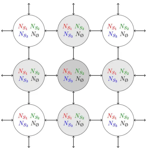
empty spaces (Ø). It has to be noted that slightly different metapopulation models of similar systems have been recently considered, see, e.g., Refs. [23,25,30,31]. As sketched in Fig.1, each patch of the array is labeled by a vectorℓ₌(ℓ1,ℓ2),

with ℓ1,2∈ {1,2, . . . ,L} and periodic boundary conditions,

and can accommodate at mostN individuals, i.e., all patches have a carrying capacity N. Each patch ℓ consists of a well-mixed (spatially unstructured) population comprising Ni(ℓ) individuals of species Si (i=1,2,3) and NØ(ℓ)=

N₋NS1(ℓ)−NS2(ℓ)−NS3(ℓ) empty spaces. SpeciesS1,S2, andS3are in cyclic competition within each patch (intrapatch

interaction), while all individuals can move to neighboring sites (interpatch mobility), see below.

The population dynamics is implemented by considering the most generic form of cyclic rock-papers-scissors-like competition between the three species with the population

FIG. 1. (Color online) Cartoon of the metapopulation model: L_×Lpatches (or islands) are arranged on a periodic square lattice (of linear sizeL). Each patchℓ₌(ℓ1,ℓ2) can accommodate at most N individuals of species S1,S2, S3 and empty spaces denoted Ø. Each patch consists of a well-mixed population ofNS1 [red (gray)] individuals of speciesS1, NS2 [green (light gray)] of typeS2, NS3 [blue (dark gray)] of typeS3andNØ=N−NS1−NS2−NS3(black) empty spaces. The composition of a patch evolves in time according to the processes (1) and (2). Furthermore, migration from the focal patch (dark gray) to its four nearest neighbors (light gray) occurs according to the processes (4), see text.

composition within each patch evolving according to the following schematic reactions:

Si+Si+1

σ

−

→Si+Ø Si+Si+1

ζ

−

→2Si, (1)

Si+Ø β

−

→2Si Si μ

−

→Si±1, (2)

where the species indexi_{∈ {}1,2,3}isordered cyclicallysuch that S3+1≡S1 and S1−1≡S3. The reactions (1) describe

the generic form of cyclic competition where Si dominates

over Si+1 and is dominated by Si−1. They account for

the dominance-removalselection processes (with rate σ) of Refs. [15,21], as well as thedominance-replacementprocesses (with rate ζ) studied notably in Ref. [16]. The process of dominance-removal accounts for cyclic dominance where speciesSi displacesSi+1 that is replaced by an empty space,

while in thedominance-replacementprocessSi+1is replaced

by an Si. This implies that dominance-replacement is a

zero-sum process conserving the total population size, whereas dominance-removalcreates empty spaces. The processes (2) allow for the reproduction of each species (with rate β) independently of the cyclic interaction provided that free space (Ø) is available within the patch. Mutations of the type Si −→Si±1(with rateμ) capture the fact thatE. colibacteria

transformations [5]. From a modeling viewpoint, the mutation yields a bifurcation around which considerable mathematical progress is feasible, see Sec.IIIand Ref. [19].

A. Mean-field analysis

When N _{→ ∞}, demographic fluctuations are negligible and the population composition within each single patch is described by the continuous variablessi =Ni/Nwhich obey

the mean-field rate equations (REs) derived in AppendixA

dsi

dt =si[β(1−r)−σ si−1+ζ(si+1−si−1)]

+μ(si₋1+si₊1−2si), (3)

wheres≡(s1,s2,s3) andr≡s1+s2+s3is the total density

and, since the carrying capacity is fixed, we have used NØ/N =1−r. The REs (3) admit a coexistence fixed point

s∗ _=s∗_{(1,1,1) with s}∗_{=β/(3β+σ) that, in the presence}

of a nonvanishing mutation rate, is an asymptotically stable focus whenμ > μH = ₆₍₃βσ_β+σ) and is unstable otherwise. In

fact, the REs (3) are characterized by a supercritical Hopf bifurcation (HB) yielding a stable limit cycle of frequency close to ωH =

√

3β(σ+2ζ)

2(3β+σ) when μ < μH [19]. In different

contexts than here, HBs have been also be found in some zero-sum RPS systems [24,25]. In the absence of mutations (μ₌0), the coexistence states∗_{is never asymptotically stable}

and the REs (3) yield either heteroclinic cycles (whenμ₌0 and σ >0) [22] or neutrally stable periodic orbits (when μ₌σ ₌0) [13]. In the absence of spatial structure, finite-size fluctuations are responsible for the rapid extinction of two species in each of these two cases [14]. It is worth noting that the heteroclinic cycles are degenerate when σ >0 and ζ ₌μ₌0.

B. Dynamics with partial differential equations

Since we are interested in analyzing the spatiotemporal arrangement of the populations, in addition to the intrapatch reactions (1) and (2), we also allow individuals to migrate between neighboring patchesℓandℓ′, according to

[Si]ℓ[Ø]ℓ′ δD

−→[Ø]ℓ[Si]ℓ′,

[Si]ℓ[Si±1]ℓ′

δE

−→[Si±1]ℓ[Si]ℓ′, (4)

where pair exchange (with rateδE) is divorced from hopping

(with rate δD). In biology, organisms are in fact known

not to simply move diffusively but to sense and respond to their environment, see, e.g., Ref. [32]. Here (4) allows us to discriminate between the movement in crowded regions, where mobility is dominated by pair exchange, and mobility in diluted regions where hopping can be more efficient, and leads to nonlinear mobility when δE =δD, see below and

Refs. [19,33].

The metapopulation formulation of the model defined by (1), (2), and (4) is ideally suited for a size expansion in the inverse of the carrying capacityN of the underlying master equation [34]. As shown in AppendixA, in the continuum limit and, to lowest order, the master equation yields the following partial differential equations (PDEs) with periodic boundary

conditions:

∂tsi =si[β(1−r)−σ si−1]+ζ si[si+1−si−1]

+μ[si−1+si+1−2si]+(δE−δD)[r si−si r]

+δD si, (5)

where heresi ≡si(x,t) and the contribution proportional to

δE−δD is a nonlinear diffusive term. These PDEs give the

continuum description of the system’s deterministic dynamics on a domain of fixed size S×S defined on a square lattice comprising L_×L sites with periodic boundary conditions, whenL_{→ ∞}andx₌S(ℓ/L) such thatx_∈[0,S]2_{. In such}

a setting, the mobility rates of (4) are rescaled according toδD,E→δD,E(S_L)2 and interpreted as diffusion coefficients

(see Appendix A). However, to mirror the properties of the metapopulation lattice model, throughout this paper we use S =L. We have found that the choiceS=Lis well suited to describe spatiotemporal patterns whose size exceeds the unit spacing, as is always the case in this work. Equations (5) and (6) have been solved using the second-order exponential time differencing method with a time stepδt ₌0.125 while the number of fast Fourier transform modes ranged from 128_×128 to 8192_×8192 [35,36].

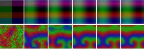
Even though the derivation of (5) assumes N _≫1 (see AppendixA), as illustrated in Fig.2(see also Ref. [19,20]), it has been found that (5) accurately capture the properties of the lattice model, whose dynamics is characterized by the emer-gence of fascinating spiraling patterns, whenN20 andμ < μH (no coherent patterns are observed whenμ > μH) [20].

WhenN ₌4–16 the outcomes of stochastic simulations are noisy but, quite remarkably, it also turns out that the solutions of (5) still reproduce some of the outcomes of stochastic simulations [19,20], see Sec.IV. In Fig.2, as in all the other figures, the results of stochastic and deterministic simulations are visualized by color (gray-level) coding the abundances of the three species in each patch with appropriate RGB intensi-ties such that [red (gray), green (light gray), blue (dark gray)]₌ (s1,s2,s3) resulting in empty spaces being color coded in black.

To next-to-leading order, the size expansion of the master equation yields a Fokker-Planck equation that can be used for instance to characterize the system’s spatiotemporal properties

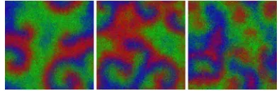
FIG. 2. (Color online) Comparison of lattice simulations (per-formed using a spatial Gillespie algorithm [37]) with solutions of (5) in the bound state phase (BS), where the spiral waves are stable, near the HB point, see text of Sec.III. Rightmost panels show the solutions of (5) while the remaining panels show results of stochastic simulations forL2₌1282_withN

in terms of its power spectra, see, e.g., Refs. [14,28]. Here, we adopt a different route and will show that the emerging spiraling patterns can be comprehensively characterized from the properties of a suitable CGLE properly derived from (5).

C. Complex Ginzburg-Landau equation

The CGLE is well known for its rich phase diagram char-acterized by the formation of complicated coherent structures, like spiral waves in two dimensions, see, e.g., Ref. [29].

In the context of spatial RPS games, the properties of the CGLE have been used first in Refs. [15] for a variant of the model considered here with only dominance-removal competition (ζ ₌μ₌0 and δD=δE). The treatment was

then extended to also include dominance-replacement com-petition (withμ₌0 andδD =δE) [17,23] and has recently

been generalized to more than three species [38]. In all these works, the derivation of the CGLE relies on the fact that the underlying mean-field dynamics quickly settles on a two-dimensional manifold on which the flows approach the absorbing boundaries forming heteroclinic cycles [13,22]. These are then treated as stable limit cycles and the spatial degrees of freedom are reinstated by introducing linear diffusion (see also Ref. [39]). While this approach remarkably succeeded in explaining various properties of the underlying models upon adjusting (fitting) one parameter, it rests on a number of uncontrolled steps. These include the approxi-mation of heteroclinic cycles by stable limit cycles and the omission of the nonlinear diffusive terms that arise from the transformations leading to the CGLE [13].

Here, we consider an alternative derivation of the CGLE that approximates (5) and describes the properties of the generic metapopulation model defined by (1), (2), and (4). Since the mean-field dynamics is characterized by a stable limit cycle (whenμ < μH) resulting from a Hopf bifurcation

(HB) arising atμ₌μH, our approach builds on a perturbative

multiscale expansion around μH (HB point). For this, we

proceed with a space and time perturbation expansion in the parameter ǫ₌√3(μH −μ) [19] in terms of the “slow

variables” (X,T)₌(ǫx,ǫ2t) [40,41]. While the details of the derivation are provided in Appendix B, we here summarize the main steps of the analysis. After the transformation

s→u=M(s−s∗_{), whereu=(u}

1,u2,u3) and M is given

by (B1),u3 decouples fromu1 andu2 (to linear order), and

one writesu(x,t)=3n=1ǫnU(n)(t,T ,X), where the

compo-nents of U(n) _{are of order O(1). Substituting into (5), with}

U₁(1)₊iU₂(1)₌A(T ,X)eiωHt_{, one finds thatAis a modulated}

complex amplitude satisfying a CGLE obtained by imposing the removal of the secular term arising at order O(ǫ3), see AppendixBand Ref. [19]. Upon rescaling Aby a constant (see AppendixB), this yields the two-dimensional CGLE with a real diffusion coefficientδ₌ 3βδE+σ δD

3β+σ as follows:

∂TA=δ XA+A−(1+ic)|A|2A, (6)

where X=∂X21+∂ 2

X2 =ǫ

−2_(∂2

x1+∂ 2

x2) and

c₌ 12ζ(6β−σ)(σ+ζ)+σ

2_(24β −σ)

3√3σ(6β₊σ)(σ₊2ζ) . (7)

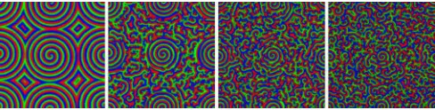
FIG. 3. (Color online) Four phases in the two-dimensional CGLE (6) forc₌(2.0,1.5,1.0,0.5) from left to right. Spiral waves of the third panel (from the left) are stable while the others are unstable, see Sec.III. Here, the colors represent the argument ofAencoded in hue: red (gray), green (light gray), and blue (dark gray), respectively, correspond to arguments 0,π/3, and 2π/3.

At this point it is worth noting the following:

(i) The CGLE (6) is a controlled approximation of the the PDEs (5) around the HB and its expression differs from those obtained in a series of previous works, e.g., in Refs. [15,17,18,23,38]. In particular, the functional dependence of the CGLE parameter (7) differs from that used in Refs. [15,17,18,23,38] for the special casesμ₌ζ ₌0 and μ₌0.

(ii) As shown in Sec.III, the phase diagram and the emerg-ing spiralemerg-ing patterns around the HB can be quantitatively described in terms of the sole parameterc, given by (7), that does not depend onμ(since hereμ_≈μH).

(iii) It has to be stressed that in the derivation of (6) no nonlinear diffusive terms appear at order O(ǫ3). In fact, the perturbative multiscale expansion yields the CGLE (6) with only a linear diffusion termδ XA, whereδ=δ(δD,δE) is an

effective diffusion coefficient that reduces toδEwhenβ ≫σ

and toδ_→δDwhenβ≪σ [19]. This implies that nonlinear

mobility plays no relevant role near the HB where mobility merely affects the spatial scale but neither the system’s phase diagram nor the stability of the ensuing patterns. Near the HB, one can therefore setδE=δD=1 yieldingδ =1 without loss

of generality.

In Secs. III and IV, we show how the properties of the CGLE (6) can be used to obtain the system’s phase diagram and to comprehensively characterize the oscillating patterns emerging in four different phases around the HB and also to gain significant insight into the system’s spatiotemporal behavior away from the HB. For the sake of simplicity we here restrictσ andζ into [0,4]. Since the components ofu=

M(s₋s∗_{) are linear superposition of the species’ densities}

andA(X,T)₌e−iωHt_(U(1)

1 +iU (1)

2 ), the modulus|A|of the

solution of (6) is bounded by 0 and 1 when one works with the slow (X,T) variables. Hence, as illustrated by Fig.3, the argument of Acarries useful information on the wavelength and speed of the patterns, whereas its modulus allows us to track the position of the spiral cores, identified as regions where_|A_{| ≈}0 corresponding to close to zero deviations from the steady states∗_{(see Fig.11below).}

III. STATE DIAGRAM NEAR THE HOPF BIFURCATION AND CHARACTERIZATION OF FOUR PHASES

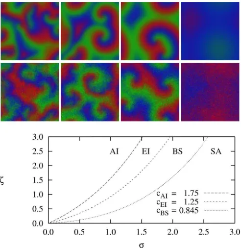
FIG. 4. (Color online) Upper panels: Typical snapshots of the phases AI, EI, BS, and SA (from left to right) as obtained from (5) (top row) and from lattice simulations (middle row) with parameters σ₌β₌δE₌δD₌1, μ₌0.02,L₌128,N=64 and, from left to right,ζ₌(1.8,1.2,0.6,0). The corresponding values of the CGLE parameter (7) are c_≈(1.94,1.47,1.01,0.63). Lower panel: Phase diagram of the two-dimensional RPS system around the Hopf bifurcation with contours ofc₌(cAI,cEI,cBS) in theσ-ζplane, see text. We distinguish four phases: spiral waves are unstable in AI, EI, and SA phases, while they are stable in BS phase. The boundaries between the phases have been obtained using (7), see Refs. [19,20] for details.

four distinct phases which can be classified in terms of the CGLE parameter c given by (7) [19,20]. As illustrated in Fig. 4, these are separated by the three critical values (cAI,cEI,cBS)≈(1.75,1.25,0.845). In theabsolute instability

(AI) phase, arising whenc > cAI, no stable spiral waves can

be sustained. In the Eckhaus instability (EI) phase, arising when cEI< c < cAI, spiral waves are convectively unstable

and their arms are first distorted and then break up. Spiral waves are stable in the bound state (BS) phase that arises when cBS< c < cEI. Spiral waves collide and annihilate in

thespiral annihilation (SA)phase when 0< c < cBS.

As illustrated by Figs.2 and 3, and in the upper panels of Fig. 4, we have verified for different sets of parameters (β,σ,ζ) andcthat the deterministic predictions of (5) and of the CGLE (6) correctly reflect the properties of the lattice metapopulation system, with a striking correspondence as soon asN 64.

In this section, Eq. (6) is used to derive the system’s phase diagram around the HB and to fully characterize each of its four phases. As explained below, the effect of noise has been found to significantly affect the dynamics only when the mobility rate is particularly low andNis of order of the unity, see Sec.IV B, but the spatiotemporal properties of the lattice model are well captured by (5) when the size of the patterns

FIG. 5. (Color online) Leftmost: Domain of size 5122 _{cut out} from a numerical solution of (5) withβ₌σ₌δD₌δE ₌1,ζ₌ 0.3,μ₌0.02, andL2₌₁₀₂₄2_{. The yellow frame outlines domain} of size 1282 _{enlarged in the middle panel. Middle: Part of a spiral} arm (far from the core) resembling a plane wave enlarged from the left panel. The color (gray color) depth of the right half of the image was reduced to 256 colors (levels of gray) for an easy identification of the wavelength found to be equal to 71 length units in the physical domain as measured by the yellow bar. Rightmost: Same as in the middle panel from lattice simulations withN₌64.

moderately exceeds that of lattice spacing, see Fig.2. In what follows, our analysis is based mainly on (6) and we have carried out extensive numerical simulations confirming that (5) and the CGLE provide a faithful description of the lattice metapopulation model’s dynamics whenN 16, while their predictions have been found to also qualitatively reproduce some aspects of the lattice simulation when N ₌2–16, see Refs. [19,20].

A. Bound-state phase (0.845c1.25)

When cBS< c < cEI, the system lies in the bound state

phase where the dynamics is characterized by the emergence of stable spiral waves that have a well-defined wavelengthλand phase velocityv. This is fully confirmed by our lattice simula-tions and by the solusimula-tions of (5), as illustrated in Fig.5where one observes well-formed spirals whose wavelengths are independent ofNandL. These quantities can be related analyt-ically using the CGLE (6) by proposing a traveling plane-wave ansatz A(X,T)₌Rei(k.X−ωT)_{, where R is the plane-wave}

amplitude. Such a traveling wave ansatz is a suitable approxi-mation away from the core of the spiraling patterns as verified in our numerical simulations. Substitution into (6) gives ω₌cR2andR2₌1₋δk2when the imaginary and real parts are equated, respectively. This yields the dispersion relation

ω₌cR2₌c(1₋δk2). (8)

This indicates that a plane wave is possible only when the wave numberk(modulus of the wave vectork) satisfies δk2<1.

We have numerically found thatk and the wavelength of the spiraling patterns vary with the system parameters, as reported in Fig. 6, where _|A|2 is shown to decrease with c in the range 0.845c1.25, with|A|2_≈R2 _{when the}

traveling wave ansatz is valid. The wavelength and phase velocity of the patterns can be obtained from the CGLE (6) and the dispersion relation (8) by noting thatk₌(1₋R2_)/δ

and thereforeλCGLE=2π/ kandvCGLE =ω/ k, see Fig.7. At

this point, it is important to realize thatλCGLE andvCGLE are

0.65 0.70 0.75 0.80 0.85 0.90 0.95 1.00

0.2 0.4 0.6 0.8 1.0 1.2 1.4

|A|

2

c

BS EI

c = 1.28

FIG. 6. Numerical values of _|A|2 _{obtained from a histogram} with 1000 bins (squares) and averaging (circles) with interpolation (dashed). When the traveling wave ansatz is valid (in BS and EI phases, away from the spirals’ cores),|A|2_≈R2_{, see text. Solid line} is the theoretical Eckhaus criterion (11) obtained from the plane-wave ansatz yieldingcEI≈1.28 marked by the dotted line. This has to be compared with the value ofcEI≈1.25 reported in the phase diagram of the two-dimensional CGLE [29]. Spiral waves are convectively unstable in the region wherec > cEI and are stable just below that value in the BS phase, see Sec.III B.

physical wavelength

λ₌ λCGLE

ǫ =

2π ǫ

δ

1−R2 (9)

and velocity

v₌ǫvCGLE=ǫcR2

δ

1₋R2. (10)

Our numerical simulations have shown that bothkand the amplitudeRof the plane wave are nontrivial functions of the CGLE parametercgiven by (7), see Fig.6. The theoretical predictions of the velocity and wavelength of the spiral waves have thus been obtained by substituting into (10) and (9) the square of the plane-wave amplitudeR2by its value computed from the solutions of CGLE (withδ₌1) as a function ofc, see Fig. 6. To this end, the numerical solutions of (6) have been integrated initially up to timet ₌799 until the spirals

0 10 20 30 40 50 60

0.6 0.8 1.0 1.2 1.4

c

SA BS EI

10 × v_CGLE

λ_CGLE

c_BS c_EI

FIG. 7. Wavelength (_◦) and (rescaled) velocity (_⋄) obtained from the CGLE (6) withδ₌1 as functions of the parameterc₌0.6–1.5. The critical valuescBSandcEIseparating the SA and BS phases and the BS and EI phases are indicated by thin vertical dotted lines, see text.

are well developed to avoid any transient effects. Then the amplitude from the successive 200 data frames between t₌ 800 andt ₌999 were averaged, yielding about 1.3_×107_data

points for each value ofc. The results (forλCGLE andvCGLE)

are summarized in Fig. 7, which shows that the wavelength decreases monotonically whencis increased (andRdecreases, see Fig. 6), with wavelengths ranging from λCGLE≈26 to

λCGLE ≈16 whencvaries from 0.845 to 1.25. By combining

this result withc’s dependence on the parameters σ and ζ, this leads to the conclusion that near the HB the wavelength of the spiral waves increases with σ and decreases with ζ, which was confirmed by our simulations (see, e.g., Fig.4). It is worth noting that in a number of earlier works withμ₌0, the quantitiesλandvwere considered to not vary with the CGLE parameterc, see, e.g., [15,17,23]. The prediction (9) can be used to theoretically estimate the spiral wavelength, see, e.g., Fig. 9 (left). As an example, the parameters used in Fig.5

correspond toc_≈0.8 andǫ_≈0.255, and therefore (9) yields λCGLE ≈27.1 and a physical wavelength λ≈27.1/0.255≈

106.3. Yet, as the example in Fig.5is not particularly close to the HB (ǫ_≈0.255), the wavelength found in the simulations is shorter than the prediction of (9). In the next section, we will see that a more accurate estimate accounting for the distance from the HB leads toλ_≈71.4, which is in excellent agreement with the numerical solutions of (5) as well as with the lattice simulations of the metapopulation model, see Fig.5(right).

Figure7also shows that, near the HB, the spiral velocity varies little within the bound state phase, with values decaying fromvCGLE≈3.0 tovCGLE≈2.7 whencvaries from 0.845 to

1.25 andδ₌1.

B. Eckhaus instability phase (1.25c1.75) As shown in Figs. 6and7the amplitude of the traveling wave solution (when it is valid) and the spirals’ wavelength vary with c. As a consequence, the wavelength decreases when c increases and above a critical value cEI the spiral

waves become unstable, see Fig. 8. Here, we demonstrate the predictive power of our approach by deriving cEI from

our controlled CGLE (6) and by characterizing the convective Eckhaus instability arising in the rangecEI< c < cAI.

WhencEI< c < cAI, small perturbations of the spiraling

patterns, which normally decay for c < cEI, grow and are

FIG. 9. Wavelengths of well-developed spiral wave solutions of the CGLE (6) withδ₌1 in the BS and EI phases (argument of Aencoded in grayscale). Here, the wavelengths are measured by counting pixels. Left: c₌1.0 and spirals are stable (BS phase). The measured wavelength is 20.2 and compares well with the theoretical predictionsλCGLE≈20.3 obtained from (9) with|A|2≈ R2_{measured as 0.904. Right:c=1.5 and spirals waves are in the EI} phase, but their arms are still unperturbed. The Eckhaus instability will cause a far-field breakup further away from the core (not shown here, see text and Fig.8). The measured wavelength of 13.8 is in excellent agreement with λCGLE≈13.7 from (9) with|A|2≈R2 measured as 0.791.

convected away from the cores; this is the Eckhaus instability, as illustrated in Fig.8. These instabilities eventually cause the far-field breakup of the spiraling patterns and the emergence of an intertwining of smaller spirals, see Fig.8(rightmost). Before the far-field breakup occurs the properties of spirals far from the core are still well described by the plane-wave solution of the CGLE (6) and the dispersion relation (8). In particular, Fig.9illustrates that the spiral wavelength relatively close to their cores (absence of far-field breakup), but still at a sufficient distance from them for the traveling wave ansatz to be valid, is in excellent agreement with the theoretical prediction (9), see also Fig.8(leftmost).

The convective nature of the instability makes it challenging to determine the critical valuec₌cEImarking the onset of the

Eckhaus instability, but its theoretical value can be predicted by considering a perturbation of the plane-wave ansatzA₌ (1₊ρ)Rei(k.X+ωT+ϕ) with_|ρ_|,_|ϕ_{| ≪}1 as a solution of our CGLE (6). Substituting this expression into (6) and seeking for a solution of the form ρ_∼ϕ_∼egT+iq.X _{[42], we find}

that Re(g)>0 and the perturbation grows exponentially when δk2>(3₊2c2)−1_{or, equivalently, when}

R2<2(1+c

2₎

3₊2c2 . (11)

In Fig.6, the criterion (11) is used to determine the onset of the EI phase by plotting the measured|A|2≈R2dependence onc in the rangec₌0.1–1.5, yielding the estimatecEI≈1.28 that

agrees well with the valuecEI≈1.25 reported in the phase

diagram of the two-dimensional CGLE [29]. The following condition on the spiral wavelengths in the physical domain of the PDEs (5) can be obtained from (9) and (11),

λ < 2π ǫ

δ(3₊2c2_{). (12)}

This gives an upper bound λEI≈5π √

δ/ǫ for the spiral wavelength in the EI phase near the HB. We note that the wavelength in Fig.8is indeed belowǫλEI.

It is worth noting that for the model withμ₌0,δD =δE,

andζ ₌1, the authors of Ref. [17] observed the occurrence of an Eckhaus instability below a certain thresholdσ derived from an uncontrolled CGLE withN ₌1. We also note that our

metapopulation model (N_≫1) predicts not only the existence of Eckhaus instability but also an absolute instability phase at low values ofσ, which has not been reported in Ref. [17].

C. Spiral annihilation phase (0<c0.845)

Whenc < cBS near the HB, the spatiotemporal dynamics

is characterized by the pair annihilation of colliding spirals. The phenomenon of spiral annihilation drives the system towards an homogeneous oscillating state filling the entire space in a relatively short time for low values ofc_≪cBS. This

phenomenon is not affected by fluctuations and not caused by any type of instabilities but is a genuine nonlinear effect and is predicted by the phase diagram of the two-dimensional CGLE [19,29]. For this reason it has not been observed in studies of models, like those of Refs. [15,17,23], not characterized by a Hopf bifurcation.

Theoretical results on the properties of the CGLE have established that in the SA phase the stable equilibrium distance between two spirals increases asymptotically as the value of cis lowered tocBS which marks the end of the bound state

phase [29]. In other words, unless the two spirals are separated by an infinite distance, they are destined to annihilate for any valuesc < cBS. The mean time necessary for the annihilation

of two spirals separated by a certain distance increases asymptotically as the value ofcapproachescBSfrom below.

Atc₌cBSit takes an infinite time for the spirals to annihilate.

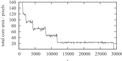
An insightful way to characterize the SA phase consist of tracking the decay of the spiral core area in time. Spiral core area here refers to the number of points on the discrete grid forming the spiral core. To efficiently measure the spiral core area, we have used the modulus of the solution of the CGLE (6). We have confirmed that|A|2_{is of orderO(1) when there are}

traveling waves (see Figs.6and3), but_|A_|2_{drops rapidly to 0}

within the small area of the core with such an area remaining approximately constant for a single core. The measure of the total core area is therefore a suitable quantity to characterize spiral annihilations. Practically, we have considered all points for which_|A_|2 _{<0.25, as being part of spiral cores (dark pixels}

in Fig.11) and the total spiral core area is the number of all such points. We have also considered other limits such as_|A_|2_<0.1

20 40 60 80 100 120 140 160

0 5000 10000 15000 20000 25000 30000

total core area / pixels

t

FIG. 11. (Color online) Spiral annihilation in the solutions of the CGLE (6) with c₌0.1 and δ₌1. The square modulus _|A_|2 _is visualized here with dark pixels representing_|A_|2_{≈0 while light} pixels show regions where|A|2_{≈1. Snapshots are taken at times} t₌(1800,2000,2200,2400,2600) from left to right.

and_|A_|2_{<0.5 finding similar behavior for all cutoffs which}

are not too close to 1. The actual value of the cutoff affects only the transients and not the long-term dynamics dominated by the increasingly rare annihilation events.

The spiral annihilations manifest themselves as sharp drops in the total core area equal to the area of the two colliding cores, as illustrated in Fig. 10 where the initial transient is characterized by a continuous decrease in the core area and the periods between first collisions are notably shorter since more spirals are present in the domain. Similarly, the time separating two successive annihilations takes always longer and the final annihilation takes longest (since spirals then need to cross the domain to collide and need to spin in opposite directions in order the annihilate). A visual representation of spiral annihilation forc₌0.1 is shown in Fig.11, where_|A|2

is coded in grayscale. Four pairs of dark spots, signifying the spiral cores with _|A_|2

≈0, are shown colliding and disappearing after approximately 3000 time steps, which is an order of magnitude less than in Fig.10forc₌0.4. It has to be noted that the time to annihilation grows ascapproaches cBS from below, as we confirmed in our simulations. While

the spiral annihilation time tends to infinity whenc_→cBS,

here the closest value tocBSthat we considered wasc=0.4

for which spiral annihilation typically occurs after a time exceeding 105_{time steps.}

D. Absolute instability phase (c1.75)

When the value of the CGLE parameter exceedsc > cAI≈

1.75 the instability occurring in the EI phase is no longer moving away from the core with the speed of the spreading perturbations exceeding the speed at which the spirals can convect them away. As illustrated in Fig.12, whenc > cAI,

FIG. 12. (Color online) Spatial arrangements in the EI (left) and AI (center, right) phases as obtained from lattice simulations near the Hopf bifurcation. Parameters areσ ₌β₌δE₌δD₌1, μ₌0.02, L₌128, N₌64, withζ ₌1.2 in the EI phase (left) andζ₌(1.8,2.4) in the AI phase (center, right). While the spatial arrangement is still characterized by (deformed) spiraling patterns in the EI phase, no spiraling arms can develop in the AI phase resulting in an incoherent spatial structure.

the perturbations grow locally, destroying any coherent forms of spiraling patterns causing their absolute instability.

From the phase diagram Fig.4we infer that the AI phase is the most extended phase (at least near the HB) and spiral waves are generally unstable whenζ _≫σ, i.e., the rate of dominance-replacement greatly exceeds that of dominance-removal. This result can be compared with the absence of stable spiral waves reported in variants of the two-dimensional zero-sum model, see, e.g., Ref. [18] (whereN ₌1 andσ ₌μ₌0).

IV. SPATIOTEMPORAL PATTERNS AND PHASES AWAY FROM THE HOPF BIFURCATION

(LOW MUTATION RATE)

While the spatiotemporal properties of the metapopulation model are accurately captured the CGLE (6) in the vicinity of the Hopf bifurcation (whereǫis small), this is in principle no longer the case at low mutation rateμ, when the dynamics oc-curs away from the Hopf bifurcation point. Yet, in this section we show how a qualitative, and even quantitative, description of the dynamics can be obtained from the CGLE (6) also when the mutation rate is low or vanishing, a case that has received significant attention in recent years [15,17,18,21,23,30].

A. Phases and wavelengths at low mutation rate

As reported in Fig. 13, it appears that three of the four phases predicted by the CGLE (6) around the HB are still present far from the HB. Here, we first explore each of these phases. As illustrated in Figs.13and12, when the rateζ is decreased from a finite value to zero at fixed low mutation rate μ (withσ, β,δD, and δE also kept fixed), the system

is first in the absolute instability (AI), then in the Eckhaus instability (EI) phase, and eventually in the bound state (BS) phase. Whenζ _≫σ and cyclic competition occurs mainly via dominance-replacement, AI in which spiral waves are unstable is the predominant phase, as observed in Refs. [18–21]. The EI and BS phases are also present near the HB and their common boundary is still qualitatively located as in the phase diagram of Fig. 4. We have noted that, similarly to what happens near the HB, the onset of convective Eckhaus-like instability is accompanied by a decrease in the wavelength with respect to the BS phase and this appears to hold even beyond the regime of validity of the CGLE approximation. The major effect on the phase diagram of loweringμat fixed

10 15 20 25 30

0.000 0.005 0.010 0.015 0.020 0.025 0.030 0.035 0.040 0.045

λCGLE

ζ = 0.2

ζ = 0.4

ζ = 0.6

ζ

µ

= 0.8

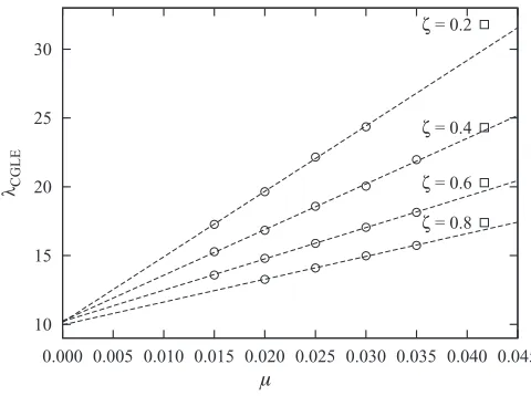
FIG. 14. Dependence ofλCGLE=ǫλon the vanishing mutation rateμfor various values ofζ: Near the Hopf bifurcationμμH _≈ 0.042, the wavelengths () are obtained from the CGLE according to (9). For lower values of μ, the wavelengths (_◦) are measured in the solutions of (5), see text. When μ_→0, λ approaches a valueλ(σ,δD,δE), see text. Parameters are as follows:σ ₌β₌δE ₌ δD₌1.

σ, whenζ is sufficiently low, is the replacement of the spiral annihilation phase by what appears to be an extended BS phase (see Fig.13, rightmost): Away from the HB and for low values ofμandζ, as in Ref. [15], instead of colliding and annihilating spiral waves turn out to be stable for the entire simulation time [43]. However, it has also to be noted that when the dominance rate σ considerably exceeds the other rates, an Eckhaus-like far-field breakup of the spiral waves occurs, see Sec.IVB.

The AI, EI, and BS phases at low mutation rates are characterized by the same qualitative properties as those studied in Sec.III(compare the upper panels of Fig.4 with Fig. 13). As a significant difference, however, it has to be noted that the wavelength of the spiraling patterns in the BS and EI phases are shorter at low mutation rates than near the HB. To explore this finding we have studied how the wavelength depends on μ. We have thus investigated how (9) can be generalized at low values ofμ. To this end, the wavelengths of the spiral waves solutions of (5) were measured forμranging from 0.015 to 0.035 and for various values of ζ (σ and β₌1 are kept fixed). As shown in Fig. 14, the measured wavelength were compared with those obtained with (9) whenμ₌μH and were found to be aligned, with a

slope that decreases whenζis increased. Quite remarkably, the values ofλcollapse towards a single wavelengthλ_→λwhen μ₌0, whereλ₌λ(σ,δD,δE) is a function of the nonmutation

ratesσ,δD,δE(whenβis fixed). These results, summarized in

Fig.14, indicate thatλdepends linearly onμ. NearμμH

the expression (9) obtained from the CGLE (6) is a good approximation for the actualλ, whereas (9) has to be rescaled by a linear factor, depending onσ,ζ, andδD,E, to obtain the

wavelength whenμ_≈0.

The general effect of loweringμis therefore to reduceλ and hence to allow to fit more spirals in the finite system. As an example, the results reported in Fig.14can be used together with (9) to accurately predict that the actual wavelength at

FIG. 15. (Color online) Effects of nonlinear mobility on spiraling patterns at zero mutation rate for various values ofδDatδEfixed. Lat-tice simulations for the metapopulation model withN₌256,L2₌ 5122_{,ζ=μ=0,σ =β=1,δE=0.5, andδD=(0.5,1,1.5,2) from} left to right. Spiral waves are stable and form geometric patterns when δD₌δE (leftmost, linear diffusion), and Eckhaus-like instability occurs when δD> δE and cause their far-field breakup, resulting in a disordered intertwining of small spiraling patterns of short wavelengths, see text.

μ₌0.02 isλ_≈71.4, which agrees excellently with what is found numerically (see Fig.5).

B. How does mobility and the rate of dominance influence the size of the spiraling patterns?

Since we have introduced mobility by divorcing pair exchange from hopping, yielding nonlinear diffusion in (5), we are interested in understanding how mobility influences the size of the spiraling patterns.

In Sec.III, we have seen that only linear mobility, via an effective linear diffusion term in (6), matters near the HB. The latter does not influence the stability of the spiraling patterns but sets the spatial scale: changing the effective diffusion coefficient δ_→αδ (α >0) rescales the space according to

x_→ x/√α, as confirmed by numerical results. A more intriguing situation arises far from the HB, where the use of the CGLE is no longer fully legitimate: Nonlinear mobility is thus found to be able to alter the stability of the spiral waves (in addition to influence the spatial scale). As illustrated by Fig.15, when the intensity of nonlinear mobility is increased (by raisingδD at fixedδE) in the BS phase, the spiral waves

that were stable under linear diffusion (see Fig.15, leftmost) disintegrate in an intertwining of spiral waves of limited size and short wavelength. It thus appears that nonlinear mobility promotes the far-field breakup of spiral waves and enhances their convective instability via an Eckhaus-like mechanism resulting in a disordered intertwining of small spiraling patterns, see Fig.15(rightmost). Furthermore, since the dominance-removal reaction is the only process that creates empty spaces that can be exploited by individuals for hopping onto neighboring patches, we expect that nonlinear mobility would be stronger at high value ofσ and for sufficiently high hopping rateδD [45].

As already noticed in Ref. [44] for a version of the model (with ζ ₌μ₌0, δD =δE, and N =1) considered here, it

FIG. 16. (Color online) Raising σ away from HB cause in-stability: Lattice simulations for the metapopulation model with N₌64,L2₌₅₁₂2_{, ζ=μ=0, β=1, δ}

D=δE =0.5, and σ = (1,2,3,4) from left to right. While the spiral waves are stable and form a geometrically ordered whenσ ₌1 (leftmost panel), Eckhaus-like instability occurs whenσis raised and cause their far-field breakup (middle panels). When σ₌4, the ordered spiraling patterns is entirely disintegrated and replaced by a disordered intertwining of spirals of small size and short wavelengths (rightmost panel), see text.

of raising σ may seem counterintuitive since the opposite happens near the HB (see Figs. 4 and 9), in accordance with the CGLE’s predictions. As a possible explanation, we conjecture that the wavelengthλapproached whenμvanishes is a decreasing function ofσ.

So far, we have seen that the description in terms of (5) and their approximation by the CGLE (6) provide a faithful description of the spatiotemporal properties of the metapopu-lation model, which appear to be driven by nonlinearity rather than by noise when the carrying capacity is sufficient to allow a meaningful size expansion. However, when nonlinear mobility and/or the dominance-removal rates are high, the deterministic description in terms of (5) yield spiraling patterns of short wavelengths and limited size. In this case, the characteristic scale of the resulting patterns is too small to lead to coherent structures and, while the deterministic description (at high resolution) may predict a disordered intertwining of small spirals, demographic noise resulting from a low carrying capacityN typically leads to noisy patches of activity on the lattice rather than to spiraling patterns [45].

V. DISCUSSION AND CONCLUSION

In this work, we have investigated the spatiotemporal patterns arising from the cyclic competition between three species in two dimensions. For this, we have considered a generic model that unifies the evolutionary processes considered in earlier works (e.g., in Refs. [15,17,18,21,23]). Here, the rock-paper-scissors cyclic interactions between the species are implemented through dominance-removal and dominance-replacement processes. In addition to the cyclic competition, individuals can reproduce, mutate, and move, either by swapping their position with a neighbor or by hopping onto a neighboring empty space, which yields nonlinear mobility. Inspired by recent experiments on microbial communities [6,8], we have formulated a metapopulation model consisting of an array of patches of finite carrying capacity, each of which contains a well-mixed subpopulation. While movement occurs between individuals of neighboring patches, all the other processes take place within each patch. The metapopulation formulation permits a neat description of the system’s dynamics and provides an ideal setting to study the influence of nonlinearity and stochasticity.

In particular, significant analytical progress is feasible in the vicinity of the Hopf bifurcation (HB) caused by the mutation process.

By investigating the deterministic and stochastic descrip-tions of the system analytically and numerically, the main achievement of this work is to provide the detailed phase diagram of a generic class of spatial rock-paper-scissors games along with the comprehensive description of the spiraling patterns characterizing the various phases. Our main analytical approach relies on the model’s CGLE derived from a multiscale perturbative expansion in the vicinity of the system’s HB. As a major difference with respect to what was done in the vast majority of earlier works on this subject, our CGLE provides us with a fully controlledapproximation of the dynamics around the bifurcation point. We have been able to exploit the well-known properties of the CGLE to obtain the accurate phase diagram near the HB in terms of a single parameter. The diagram is characterized by four phases, called “absolute instability” (AI), “Echkaus instability” (EI), “spiral annihilation” (SA), and “bound state” (BS). Spiral waves are found to be stable and convectively unstable in the BS and EI phases, respectively, where their wavelength and velocity have been obtained from the dispersion relation of the CGLE and found to be in good agreement with results of both the deterministic and lattice simulations of the system. We have also been able to derive the threshold separating the BS and EI phases. The SA phase, whose existence is found to be limited to the vicinity of the HB, is characterized by the spiral waves’ annihilation time (inferred from the CGLE). Finally, we have found that there is always a regime (AI phase), typically arising when dominance-replacement outcompetes dominance-removal, where any coherent form of spiraling patterns is prevented by growing local instabilities. We have also been able to take advantage of the CGLE to analyze the model’s spatiotemporal properties at low mutation rates, i.e., far from the HB. In particular, we have found that at low mutation rate the AI, EI, and BS phases are still present, whereas the SA phase is replaced by what appears to be an extended BS phase. We have found that the wavelength of the spiral waves in the BS and EI phases decays linearly with the mutation rate. While we have focused on the two-dimensional system for its biological relevance, it worth noting that our analytical approach based on the CGLE is general and can also cover the cases of one and three spatial dimensions: One would then obtain different phase diagrams wherein which one would notably find traveling waves (in one dimension) and scroll waves (in three dimensions) instead of instead of spiraling patterns.

In general, we have seen that phenomena like far-field breakup and convective instabilities that characterize the EI phase, and limit the size of the spirals as well as their coherent arrangement, can also be caused by nonlinear mobility and by high dominance-removal rate. Under high nonlinear mobility or for high dominance-removal rate, the system may exhibit spiraling patterns of short wavelength and limited size even in the extended BS phase. In this case, if the carrying capacity is low, the intensity of demographic noise may prevent the visualization of spiraling patterns on the discrete lattice [45].

coexistence of cyclically competing species in a generic two-dimensional rock-paper-scissors system are stable and persist, we expect that our findings can contribute to shed further light on the spatiotemporal arrangements of population in cyclic competition. For instance, our findings provide various theoretical scenarios for the lack of observation of spiraling patterns in microbial experiments as those of Ref. [6], that it would be interesting to test experimentally. One possible explanation could be that the experimental parameters would correspond to a regime where spiral waves are unstable. Another plausible explanation could be that the time scale on which the experiments of Ref. [6] have been carried out (several days) is much shorter than the time necessary for the formation of spiraling patterns in the simulations of the model. This would imply that spiraling patterns would take very long (perhaps several months) to form on a Petri dish, which might explain why they have remained elusive. We also believe that our theoretical results can potentially serve to guide further experimental investigations on microbial communities, like those of Ref. [6], by predicting parameter regimes where species coexistence could form spiraling patterns as in myxobacteria and in dictyostelium mounds [26].

ACKNOWLEDGMENTS

B.S. is grateful for the support of the EPSRC (Grant No. EP/P505593/1).

APPENDIX A: STOCHASTIC DYNAMICS AND VAN KAMPEN SIZE EXPANSION

In this appendix, we explain how the stochastic dynamics of the generic metapopulation models (1)–(4) can be captured by the system’s master equation. We also outline how the latter can be expanded to yield a more amenable description of the dynamics [34].

1. Master equation

We here derive the master equation (ME) governing the stochastic dynamics of the generic metapopulation model. Combining the reaction rates with appropriate combinatorial factors, the transition probabilities for each intrapatch reac-tions (1) and (2) can be written as

T_iβ(ℓ)₌βNSi(ℓ)NØ(ℓ)

N2 , (A1)

T_iσ(ℓ)₌σNSi(ℓ)NSi+1(ℓ)

N2 , (A2)

T_iζ(ℓ)₌ζNSi(ℓ)NSi+1(ℓ)

N2 , (A3)

T_iμ(ℓ)₌μNSi(ℓ)

N . (A4)

The combinatorial factors, such asNSi(ℓ)NSi+1(ℓ)/N

2_{, express}

the probability of species Si and Si+1 to interact within a

patch at site ℓ. The same applies to NSi(ℓ)NØ(ℓ)/N

2 _for

the probability of species Si encountering an empty space

denoted by Ø. Migration between two neighboring patches

occurs by pair exchange (with rateδE) and by hopping (with

rateδD) according to (4), which similarly yields the transition

probabilities

DδD

i (ℓ,ℓ′)=δD

NSi(ℓ)NØ(ℓ′)

N2 , (A5)

DδE

i (ℓ,ℓ′)=δE

NSi(ℓ)NSi±1(ℓ′)

N2 . (A6)

At this point, it is useful to introduce the step-up and step-down operators [34]. These act on a given state or transition by changing the numbers of individuals by_±1, i.e.,E±i NSi(ℓ)= NSi(ℓ)±1 and therefore

E±i (ℓ)T β i (ℓ)=β

NSi(ℓ)±1

NØ(ℓ)

N2 . (A7)

This allows the total transition operator for intrapatch reactions to be written as

Ti(ℓ)=[E+i+1(ℓ)−1]T

σ

i (ℓ)+[E−i (ℓ)E+i+1(ℓ)−1]T

ζ i (ℓ)

+[E−i (ℓ)−1]T β i (ℓ)

+[E−i (ℓ)E+i+1(ℓ)+E−i (ℓ)E+i−1(ℓ)−2]T

μ

i (ℓ). (A8)

The general form of the terms [E±

...−1]T...originates from

the gain and loss terms in probability to find the system in a particular state. Correspondingly, the total migration operator for diffusions between neighboring subpopulations reads

Di(ℓ,ℓ′)=[Ei+(ℓ)E−i (ℓ′)−1]D δD i (ℓ,ℓ′)

+[E+i (ℓ)E−i±1(ℓ)Ei−(ℓ′)E+i±1(ℓ′)−1]D

δE i (ℓ,ℓ′).

(A9)

Finally, we can write the master equation for the probability P(N,t) of a system occupying a certain state N at time t by summing the operators over all species i_{∈ {}1,2,3_} and subpopulationsℓ_{∈ {}1, . . . ,L_}2, which yields

dP(N,t)

dt =

3

i=1

L×L

ℓ

Ti(ℓ)+

1 2

±

ℓ′_∈ℓ

Di(ℓ,ℓ′)

P(N,t).

(A10)

Here the termℓ′_{∈ℓindicates summation over all neighbors}

of patch ℓ and _± denotes the sum over i_±1 in (A9). In addition, N_{= {}NØ(ℓ),NSi(ℓ)|i=1,2,3,ℓ∈L×L}is

de-fined as a collection of allNSi(ℓ)’s and empty spacesNØ(ℓ) in

all subpopulations specifying uniquely the state of the entire system. Later,ηis used to symbolize a similar collection for fluctuationsηi(ℓ) defined below.

2. System size expansion

While the mathematical treatment of (A10) represents a formidable problem, significant progress can be made by performing an expansion in the inverse of the carrying capacity N [34]. Such a system size expansion requires the introduc-tion of new rescaled variables. The normalized abundances (densities) of species are equal to si(ℓ)=Ni(ℓ)/N. Here,

with√Nsuch that

ηi(ℓ)=

√

N[s∗₋si(ℓ)], wheres∗=

β

β₊3σ, (A11)

which after differentiating with respect to time becomes

dηi(ℓ)

dt = −

√

Ndsi(ℓ)

dt . (A12) With this assumption, it is now possible to write the master equation for a (redefined) probability density(η,t) in terms of the fluctuations ηi(ℓ). As usual, the time is rescaled as

t_→t /Nand the left-hand side of (A10) thus becomes

1 N

∂(η,t)

∂t −

3

i=1

{1,...,L}2

ℓ 1

√

N dsi(ℓ)

dt

∂(η,t)

∂ηi(ℓ)

. (A13)

The right-hand side of (A10) can be written in a similar way by introducingsi(ℓ) andηi(ℓ) variables. The up and

step-down operators are also expanded in their differential form which, up to the orderO(N−1_{), reads}

E±i (ℓ)=1±

1

√

N ∂ ∂ηi(ℓ)+

1 2

1 N

∂2

∂η2_i(ℓ). (A14)

The results of successive application of the operators can be obtained by multiplying their differential forms. For example, the application ofE+i (ℓ)E−i (ℓ′) results in

E+i(ℓ)E−j(ℓ′)=1+

1

√

N

_∂

∂ηi(ℓ) −

∂ ∂ηj(ℓ′)

+ 1 2 1 N ∂ ∂ηi(ℓ)−

∂ ∂ηj(ℓ′)

2

. (A15)

After some algebra, the terms at the same order ofN can be collected on both sides of the master equation (A10). At order O(N−1/2_{), the leading terms describe the time evolution of}

the species densitiessi(ℓ). Leaving out the migration terms for

now and collecting all intrapatch reaction terms, the ordinary differential equations describing changes in one patch can be written down. These mean-field equations are also referred to as the rate equations. Since only the subpopulation in one patch is considered at this point and space is currently irrelevant, the spatial variable ℓ insi(ℓ) is temporarily dropped. With the

introduction ofs=(s1,s2,s3) andr=s1+s2+s3, the ODEs

read dsi

dt =si[β(1−r)−σ si−1+ζ(si+1−si−1)]

+μ(si−1+si+1−2si)=Fi(s), (A16)

which corresponds to the mean-field rate Eqs. (3).

When migration terms are accounted for, the size expansion to orderO(N−1/2_{) yields terms that describe the deterministic}

spatial dynamics of the model. In the suitable continuum limit, these lead to the following partial differential equations (PDEs) for the continuous coordinatex ₌S(ℓ/L) describing the system’s dynamics on a domain of sizeS:

∂si(x)

∂t =Fi(s(x))+δD

S

L

2

si(x)+(δD−δE)

S

L

2

× [si(x) r(x)−r(x) si(x)], (A17)

where Fi(s(x)) in the first line coincides with the

right-hand side of (A16) where the spatial dependence of the densities is reinstated according tosi →si(x). At this point,

it is useful to comment on the derivation and interpretation of (A17), which coincides with (5). To lowest order, the size expansion of the master equation with migration yields terms like δD[ℓ′_∈ℓsi(ℓ′)−4si(ℓ)], where ℓ′ are the four

nearest neighbors to site ℓ. To obtain the deterministic description of the model in the continuum limit on a domain of fixed sizeS×S, we consider the number of lattice sites L_{→ ∞}. In terms of the variable x₌(x1,x2), the mobility

rates of (4) are thus rescaled according toδD,E→δD,E(S_L)2

and interpreted as diffusion coefficients. Therefore, in the continuum limit δD[ℓ′_∈ℓsi(ℓ′)−4si(ℓ)]→δD(S_L)2 si(x),

where the differential operator =∂2

x1+∂ 2

x2 is the usual two-dimensional Laplacian. For the sake of comparison with lattice simulations, we set the domain size to be equal to the lattice size, i.e.,S₌Lso the diffusion coefficients coincide with the mobility rates. It is important to note that apart from the nonspatial ODEFi(s(x)) (A16) and a linear diffusive term

δD si(x) there are also additional nonlinear diffusive terms

appearing in the second line of (A17). These vanish only in the case ofδD =δE considered in the vast majority of other

studies, e.g., in Refs [15,17,18,23].

APPENDIX B: MULTISCALE EXPANSION AND COMPLEX GINZBURG-LANDAU EQUATION

In this Appendix, we provide details of the multiscale asymptotic expansion leading to the complex Ginzburg-Landau equation (6) which provides a controlled (perturbative) approximation of the model’s dynamics in the vicinity of the Hopf bifurcation.

1. Linear transformations

Before performing the asymptotic expansion can be per-formed, it is convenient to work with the shifted variables

u=(u1(x),u2(x),u3(x))=M(s−s∗), where

M= √1

6 ⎛ ⎜ ⎝

−1 ₋1 ₋2

−√3 √3 0

√

2 √2 √2 ⎞ ⎟

⎠. (B1)

With this transformation, the origin coincides with the fixed point s∗_{. In these new variables, the linear part of the rate}

equations (A16) are in the Jordan normal form as follows:

du(x)

dt =

⎡ ⎢ ⎣

ǫ ₋ωH 0

ωH ǫ 0

0 0 −β ⎤ ⎥

⎦u(x), (B2)

where β is the reproduction rate, ωH = √

3β(σ+2ζ) 2(3β+σ) , ǫ= √

3(μH−μ), and μH = βσ

6(3β+σ). One notices that u3(x)

decouples from the oscillations in the u1(x)-u2(x) at Hopf

frequency ωH. The dynamics of three species abundances is