University of Southern Queensland
School of Mechanical and Electrical Engineering
Investigation of Refrigeration System Steam Ejector
Performance Through Experiments and Computational
Simulations
A thesis submitted by
Ghassan Fadil Lattif Al-Doori
in fulfilment of the requirements of
Doctor of Philosophy
iii
اَنْيَّص َو َو
َناَسْنِ ْلْا
ِهْيَدِلا َوِب
اًناَس ْحِإ
ۖ
هْتَلَم َح
هُّم أ
اًه ْر ك
هْتَعَض َو َو
اًه ْر ك
ۖ
ه لْم َح َو
ه لاَصِف َو
َنو ث َلََث
ا ًرْهَش
ۖ
ىَّت َح
اَذِإ
َغَلَب
هَّد شَأ
َغَلَب َو
َنيِعَب ْرَأ
ًةَنَس
َلاَق
ب َر
يِن ْع ِز ْوَأ
ْنَأ
َر كْشَأ
َكَتَم ْعِن
يِتَّلا
َتْمَعْنَأ
َّيَلَع
ىَلَع َو
َّيَدِلا َو
ْنَأ َو
َلَم ْعَأ
ا ًحِلاَص
هاَض ْرَت
ْحِل ْصَأ َو
يِل
يِف
يِتَّي ر ذ
ۖ
ي نِإ
تْب ت
َكْيَلِإ
ي نِإ َو
َنِم
َنيِمِل ْس مْلا
ميظعلا الله قدص
ميحرلا نمحرلا الله مسب
Translation
In the name of Allah, Most Gracious, Most Merciful.
Dedication
Thee my Lord to be satisfied
And then
To Dad and Mum
To my brothers and my sister
To my family Hafssa, Oras,
Othman, Faidha (Meriam), Ryaheen, Abdulrahman,
Abstract
Recently, vapour compression using ejectors has received more interest from researchers in the air conditioning and refrigeration field. Ejectors have the advantage of being extremely reliable with stable operation and no moving parts leading to essentially maintenance free operation. However, ejectors have very low efficiencies and this can be attributed to the low entrained mass flow rate of the secondary stream relative to the primary stream mass flow rate. The entrainment and mixing between primary and secondary streams is therefore a dominant feature which requires investigation. This thesis introduces and demonstrates new methods to characterise the mixing process in a vapour compression ejector operated with steam as the working fluid.
A new steam ejector refrigeration apparatus was built to visualise the mixing flow inside the ejector. New designs for the steam generator and the evaporator chamber were used in this apparatus. The evaporator chamber was developed in order to weigh the amount of water induced from the evaporator during the test time. The weighing method was demonstrated to be sufficiently accurate for this application. The highest percentage difference between the direct weighing method and a thermal method for deducing the secondary stream mass flow rate was 2.6 %, corresponding to about 0.3 % of the entrainment ratio.
sec-ii
ondary stream conditions and different condenser pressures. The difference between experimental data and the Eilmer3 simulations of static wall pressure was typically less than 2 %. The difference between experimental data and the Eilmer3 simulation of entrainment ratio was 2.9 % at 130 primary stream temperature and 2.6 % at 120primary stream temperature for choked ejector operation. For ejector operation at unckoked conditions, differences between experimental results and the simulations were substantial with the critical condenser pressure typically underestimated in the simulation by around 8.8 % at 270 kPa primary stream pressure and 15.4 % at 200 kPa primary stream pressure.
To enable visualisation of the ejector flow, a transparent acrylic duct was optically designed using a ray tracing method. The machined and polished optical duct per-formed as expected in that it provided a field of view over the entire height of the duct. However, the planned schileren visualisation could not proceed with the optical duct because of shadowing effects attributed to birefringence in the duct material. Never-theless the optical duct was successfully used to gain photographic evidence of liquid water and ice building up within the ejector. The presence of liquid and solid forms of water within the ejector suggests the ideal gas model cannot generally be applied to the steam ejector flows even though a good degree of success was achieved in modelling the static pressure distribution and entrainment ratio under choked flow conditions.
A new technique for exploring the mixing region generated by the steam ejector nozzle was introduced. The new approach used a pitot tube to measure the pressure profile at different positions downstream of the nozzle exit within a mixing chamber with a rela-tively large rectangular cross section. A special pitot probe and traversing mechanism was designed and fabricated for this purpose. The experimental results demonstrate a shock train was established downstream of the nozzle exit. The experimental measure-ments indicate that pressure wave effects within the mixing jet have largely dissipated by the 70 mm downstream location. Eilmer3 simulations were also used to investigate the flow at the nozzle exit. Eilmer3 simulations duplicate experimental pitot pressure data at the first station downstream of the nozzle exit (1 mm) but are not consistent with the pitot pressure measurements at the other positions (25, 50, and 70 mm).
at-iii
tempted. Using the Eilmer3 simulation at the nozzle exit, the momentum transport into the control volume was calculated. The momentum transport out of the control volume was the estimated using experimental data at the 70 mm station based on an ideal gas analysis and an assumed constant static pressure across the jet. To reflect possible condensation effects, values for the ratio of specific heat lower thanγ = 1.326 were trialled in the analysis in an attempt to achieve the required momentum transport out of the control volume. However, even with γ = 1.001 the momentum transport out the control volume was too high, indicating that an inflow momentum transport contribution due to recirculation across the downstream station may be significant although it was not included in the analysis.
Certification of Dissertation
I certify that the ideas, designs and experimental work, results, analyses and conclu-sions set out in this dissertation are entirely my own effort, except where otherwise indicated and acknowledged.
I further certify that the work is original and has not been previously submitted for assessment in any other course or institution, except where specifically stated.
Ghassan Fadil Lattif Al-Doori
w0095038
Signature of Candidate
Date
ENDORSEMENT
Signature of Supervisor/s
Acknowledgments
First of all I would like to thank My God, who helped me finished this thesis.
I would also like to express my grateful thanks to my supervisor Professor David Buttsworth, for his persistence, concern and support. This dissertation would not have been possible without his guidance and wisdom. It is also my pleasure to work with Dr Mike Dennis from the Australian National University as my Associate supervisor. His academic assistance improved the depth of understanding of this study. I would also like to extend my appreciation to my Associate supervisor, Dr Andrew Wandel, for his academic support.
Moreover, special recognition is also given to Dr Peter Jacobs and colleagues from the University of Queensland for their assistance.
I would like to highlight my deep appreciation for my friend Dr Rafat Al Jassim from the University of Queensland for his moral support.
Also I would like to recognize the encouragement given by my colleagues: Dr Ray Malpress, Dr Sudantha Balage, Dr Les Bowtell, Andreas Helwig, Brett Richards, Terry Byrne, Graham Holmes, and Dean Beliveau. They generously shared their expertise which undoubtedly reduced the time I required to complete several tasks.
I will never forget those who gave me good technical support Brian Aston, Chris Galligan, Jim Scott, and Kevin Airton.
vi ACKNOWLEDGMENTS
of Southern Queensland for their support.
I would like to thank Oras for her support, encouragement, and advice which helped to manage some difficult situations during my candidature.
I would like to thank Hafssa for looking after my family and her patience.
Finally, I would like to thank the Ministry of Higher Education in my country for this opportunity to finish the Doctor of Philosophy degree.
Ghassan Fadil Lattif Al-Doori
Contents
Dedication i
Abstract i
Acknowledgments vi
List of Figures xvii
List of Tables xxxiv
Notation xxxvi
Acronyms & Abbreviations xl
Chapter 1 Introduction 1
1.1 Applications of an ejector . . . 1
1.2 Ejector refrigeration systems . . . 1
1.3 Ejector operation . . . 2
viii CONTENTS
1.5 Objectives of the dissertation . . . 5
1.6 Overview of the Dissertation . . . 6
1.6.1 Chapter 2 Literature review . . . 6
1.6.2 Chapter 3 Overview of the design of the apparatus . . . 6
1.6.3 Chapter 4 System performance . . . 6
1.6.4 Chapter 5 Ejector results and discussion . . . 6
1.6.5 Chapter 6 Computational simulation . . . 7
1.6.6 Chapter 7 Mach 4 steam jet . . . 7
1.6.7 Chapter 8 Flow visualisation . . . 7
1.6.8 Chapter 9 Conclusions and future work . . . 8
Chapter 2 Literature review 9 2.1 Introduction . . . 9
2.2 Ejector performance studies . . . 9
2.2.1 Analytical work . . . 9
2.2.2 Operating conditions . . . 12
2.2.3 Primary nozzle arrangement . . . 13
2.3 Flow visualisation studies . . . 15
2.4 Computational fluid dynamics simulations . . . 18
CONTENTS ix
Chapter 3 Overview of the design of the apparatus 26
3.1 Introduction . . . 26
3.2 Apparatus layout . . . 27
3.3 Steam ejector . . . 27
3.3.1 Primary nozzle . . . 32
3.3.2 Secondary inlet . . . 38
3.3.3 Mixing chamber . . . 38
3.3.4 Diffuser . . . 40
3.4 Steam generator . . . 41
3.5 Evaporator . . . 46
3.6 Evaporator load control . . . 46
3.7 Evaporator chamber . . . 46
3.8 Condenser . . . 48
3.9 Measurement arrangement . . . 48
3.9.1 Pressure transmitter . . . 48
3.9.2 Balance . . . 50
3.10 Data acquisition . . . 50
3.11 Electrical arrangement . . . 50
3.12 Conclusion . . . 51
x CONTENTS
4.1 Introduction . . . 52
4.2 Performance of the open cycle . . . 52
4.2.1 Measurement of mass flow rate . . . 54
4.2.2 Heat loss from primary stream within the stainless steel pipe . . 57
4.2.3 Head losses from primary stream within the stainless steel pipe . 58 4.2.4 Non-electrical heat gain by the evaporator . . . 58
4.2.5 Pressure transducer electrical noise . . . 60
4.3 Preliminary test . . . 60
4.3.1 Examination of the nozzle parameters . . . 60
4.3.2 Nozzle exit position (NXP) effect on COP . . . 61
4.3.3 System stability during the test time . . . 63
4.3.4 Critical condenser pressure of the steam ejector . . . 69
4.4 Conclusion . . . 71
Chapter 5 Ejector results and discussion 72 5.1 Introduction . . . 72
5.2 Operating regimes . . . 73
5.3 Effect of primary stream conditions . . . 78
5.4 Effect of condenser pressure on pressure distributions . . . 82
5.5 Effect of evaporator load on COP . . . 85
CONTENTS xi
5.7 Conclusion . . . 90
Chapter 6 Computational simulation 91 6.1 Introduction . . . 91
6.2 Building and running simulation . . . 92
6.3 Turbulence models . . . 92
6.4 k-ω Turbulence model . . . 93
6.5 Recommendation to use k-ω model in Eilmer3 . . . 95
6.5.1 Dimensionless wall distance,y+ . . . 95
6.5.2 Number of cells within boundary layer . . . 96
6.5.3 Maximum cell aspect ratio . . . 97
6.6 Simulated ejector configuration . . . 97
6.7 Grid of the ejector in CFD . . . 99
6.8 Simulation time . . . 102
6.9 Validation of Eilmer3 simulations . . . 103
6.9.1 Validation of static pressure . . . 103
6.9.2 Validation of entrainment ratio . . . 108
6.10 Simulated pressure and velocity distributions . . . 110
6.10.1 Choked flow . . . 110
6.10.2 Unchoked flow . . . 115
xii CONTENTS
6.11 Conclusion . . . 121
Chapter 7 Mach 4 steam jet 122 7.1 Introduction . . . 122
7.2 Experimental arrangement . . . 123
7.2.1 Mixing chamber . . . 123
7.2.2 Pitot tube probe . . . 125
7.2.3 Pressure and temperature . . . 127
7.2.4 Operating procedure . . . 127
7.3 System performance during the test time . . . 128
7.3.1 Primary flow stability . . . 128
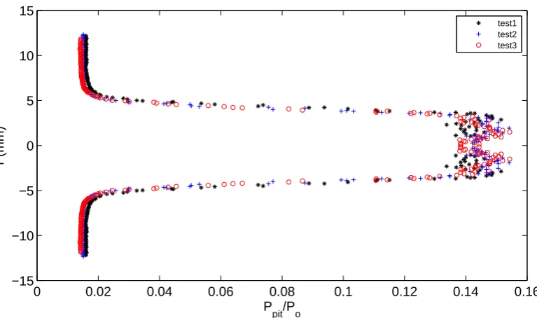
7.3.2 Repeatability of survey data . . . 130
7.4 Over-expanded jets . . . 133
7.5 Results and discussion . . . 134
7.6 Simulation using Eilmer3 . . . 139
7.6.1 Simulation of mixing chamber configuration . . . 139
7.6.2 Comparison of Eilmer3 simulations with pitot data . . . 140
7.7 Momentum integral analysis . . . 145
7.8 Conclusion . . . 149
CONTENTS xiii
8.1 Introduction . . . 150
8.2 Lens design and commissioning . . . 151
8.2.1 Overview of optical arrangements . . . 151
8.2.2 Overview of ray-tracing design . . . 152
8.2.3 Performance assessment . . . 153
8.3 Schlieren visualisation arrangement . . . 154
8.3.1 Method overview . . . 154
8.3.2 System sensitivity . . . 155
8.3.3 Experimental arrangement . . . 156
8.4 Schlieren visualisation results . . . 158
8.5 Assessment of density gradients . . . 162
8.6 Visualisation of ice formation . . . 164
8.7 Conclusion . . . 165
Chapter 9 Conclusions and future work 166 9.1 Summary . . . 166
9.2 Conclusions . . . 167
9.2.1 Ejector . . . 167
9.2.2 Computational simulation . . . 167
9.2.3 Mach 4 steam jet . . . 168
xiv CONTENTS
9.3 Future work . . . 170
References 172 Appendix A 181 A.1 Primary nozzle and spacer . . . 181
A.2 Plenum chamber . . . 183
A.3 Secondary inlet and mixing chamber 1 . . . 184
A.4 Diffuser . . . 186
A.5 Steam generator and stirrer . . . 187
A.6 Evaporator . . . 188
A.7 Evaporator controller load . . . 189
A.8 Condenser . . . 190
A.9 Electrical arrangement . . . 191
Appendix B Calculations and other supporting details on system per-formance. 194 B.1 Heat loss from primary stream within the stainless steel pipe . . . 194
B.1.1 Head losses from primary stream within the stainless steel pipe . 196 B.2 Non-electrical heat gain by the evaporator . . . 196
B.3 Experimental work procedure . . . 197
CONTENTS xv
B.3.2 Fill evaporator with water . . . 201
B.4 Dosing pump . . . 202
Appendix C Instrument calibration 204
C.1 Pressure transducers calibration . . . 204
C.2 Thermocouple calibration . . . 209
C.3 Dosing pump calibration . . . 209
Appendix D Two correcting lens designs 212
D.1 Lens design . . . 212
D.2 Case one: Separate tube and lens . . . 212
D.3 Case two: Integral tube and lens . . . 217
Appendix E Eilmer3 scripts for steam ejector. 221
E.1 Python.py file . . . 221
E.2 Shell Scripts . . . 236
List of Figures
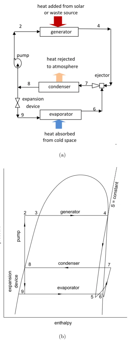
1.1 (a) Ejector pump refrigeration system; (b) Illustrative p-h diagram of a closed cycle ejector based refrigeration system. . . 3
1.2 Geometry of an ejector. . . 4
2.1 Schematic diagram of ejector (Huang, Chang, Wang and Petrenko, 1999). 10
2.2 Schematic illustration of operation regimes associated with the con-denser pressure (Pridasawas, 2006). . . 12
2.3 Primary nozzle geometries used by Chang and Chen (2000). . . 14
2.4 Configuration of steam ejector with spindle by Ma, Zhang, Omer and Riffat (2010). . . 14
2.5 Optical device, TSI atomiser and acquisition system used by Desevaux (2001b). . . 16
2.6 Comparison between experimental visualisation and numerical CFD vi-sualisation (Marynowski, Desevaux and Mercadier, 2009). . . 17
2.7 Experimental rig used by Bouhanguel, Desevaux and Gavignet (2010). . 18
LIST OF FIGURES xvii
2.9 Variation of calculated entrainment ratio of a steam ejector: effect of operating pressure (Sriveerakul, Aphornratana and Chunnanond, 2007a). 20
2.10 Filled contours of Mach number: effect of downstream pressure. All operating points A, B, C, D and E correspond to those shown in Figure (2.9) (Sriveerakul, Aphornratana and Chunnanond, 2007b). . . 21
2.11 Comparison between two turbulence models,k-and k-ω-SST, and ex-perimental data on the entrainment ratio at different primary stream pressures: (a) P1o = 3 bar, (b) P1o = 6 bar (Hemidi, Henry, Leclaire, Seynhaeve and Bartosiewicz, 2008). . . 22
2.12 Comparison between two turbulence modelsk-andk-ω-SST. Contours of the stream function for the top half of the mixing chamber (Hemidi, Henry, Leclaire, Seynhaeve and Bartosiewicz, 2009). . . 23
2.13 Nozzle shapes tested by Yang, Long and Yao (2012) (all dimensions in mm). . . 24
3.1 Schematic diagram of the steam ejector system. . . 28
3.2 Photograph of the steam ejector system. . . 29
3.3 (a) Schematic illustration of the steam ejector (b) Section A-A compres-sion fitting (c) Section T-T threaded adapter. . . 30
3.4 Illustration of steam ejector sectors considered in design. . . 31
3.5 variation of the molecular weight correction factor C1 with molecular
weight of gas (ESDU86030, 1986). . . 33
3.6 Variation of compression ratio Ns with primary pressure ratio Np and
entrainment ratioω (ESDU86030, 1986). . . 34
3.7 Variation of nozzle area ratio AT with primary pressure ratio Np for
xviii LIST OF FIGURES
3.8 (a) Overall dimensions of the nozzle, all dimensions (mm) (b) Throat
profile details. . . 37
3.9 Photographs of the perspex mixing section. (a) Converging section of the mixing chamber (b) Parallel section of the mixing chamber (c) As-sembled mixing chamber. . . 40
3.10 Diffuser made from brass. . . 41
3.11 Schematic boiler as used by Sriveerakul et al. (2007a). . . 42
3.12 Steam generator arrangement used in the present work. . . 44
3.13 Evaporator chamber. (a) Schematic illustration of arrangement; (b) Photograph of device. . . 47
3.14 Illustration of the measurement devices. . . 49
4.1 Illustrative of p-h diagram of the open cycle steam ejector. . . 53
4.2 (a) Schematic of stainless steel pipe within insulation and concentric copper pipe; (b) Cross section of region 1 and region 2. . . 57
4.3 Schematic of evaporator with armaflex insulation. . . 59
4.4 Effect of nozzle exit position on COP for primary stream stagnation conditions of 130 and 270 kPa. . . 62
LIST OF FIGURES xix
4.6 (a) Fluctuations of the evaporator pressure during the test time for three loads 3500 W, 2500 W and 1200 W. (b) Corresponding fluctuations of the secondary flow temperature during the test time. Result for NXP = -32 mm. . . 65
4.7 Fluctuations of the condenser pressure during the test time for NXP = -32 mm, and conditions corresponding to Figure 4.6. . . 66
4.8 (a) Geometric arrangement of the ejector; (b) Pressure variation with distance along the ejector with error bars indicating the temporal pres-sure variations recorded for 100 samples during 10 second; (c) Corre-sponding results for the case of 6000 samples during 10 minutes, primary stream pressure of 270 kPa and evaporator load of 1200 W. . . 68
4.9 (a) Condenser pressure change during the test time; (b) Evaporator pressure change during the test time; (c) Evaporator temperature change during the test time . . . 70
5.1 Illustrative variations of pressure during apparatus operation. Eventu-ally the evaporator pressure increases in response to an increase in the condenser pressure whereas no change of the primary stream pressure occurs during the transition from choked flow to reverse flow regions. . . 73
5.2 Experimental results over a range of condenser pressures for an evap-orator load of 3000 W with primary stream conditions of 270 kPa and 130(a) COP of steam ejector; (b) Evaporator temperature variation. 75
5.3 Experimental results over a range of condenser pressures for an evapora-tor load of 2000 W with primary stream conditions of 200 kPa, 120(a) COP of steam ejector; (b) Evaporator temperature variation. . . 76
xx LIST OF FIGURES
5.5 COP variation with condenser pressure for primary stream pressures of 270, 200, and 143 kPa and corresponding temperatures of 130, 120, and 110 with 3000 W cooling load. . . 79
5.6 COP variation with condenser pressure for primary stream pressures of 270, 200, and 143 kPa and corresponding temperatures of 130, 120, and 110 with 2000 W cooling load. . . 79
5.7 COP variation with condenser pressure for primary stream pressures of 270, 200, and 143 kPa and corresponding temperatures of 130, 120, and 110 with 1000 W cooling load. . . 80
5.8 Entrainment and mixing process in the mixing chamber (a) Long en-trainment duct; (b) Short enen-trainment duct (Chunnanond and Aphorn-ratana, 2004). . . 80
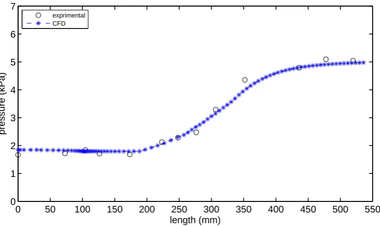
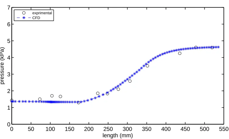
5.9 Static pressure along the ejector wall for primary stream pressures of 270 kPa, 200 kPa and 143 kPa, and corresponding temperatures of 130, 120, and 110for an evaporator temperature of 14 and a 4.2 kPa condenser pressure. . . 82
5.10 Static pressure along the ejector wall for primary stream pressure of 270 kPa, and corresponding temperature of 130for an evaporator tem-perature of 14 and 3.6 kPa, 4.4 kPa, 5.5 kPa, and 6.8 kPa condenser pressures. . . 83
5.11 Static pressure along the ejector wall for primary stream pressure of 200 kPa, and corresponding temperature of 120for an evaporator tem-perature of 14 and 3.6 kPa, 4.3 kPa, 5.4 kPa, and 6.1 kPa condenser pressures. . . 84
LIST OF FIGURES xxi
5.13 Experimental results displaying the effects of evaporator load on the COP of the ejector for condenser pressures sufficiently low to achieve choked secondary stream conditions. . . 85
5.14 Static pressure along the ejector wall for different evaporator temper-atures at 4 kPa condenser pressure and a primary stream pressure of 270 kPa and temperature 130. . . 86
5.15 COP results from previous studies compared with those of the present work for a primary stream temperature of 130 and an evaporator temperature of 15. . . 87
5.16 COP results from previous studies compared with those of the present work for a primary stream temperature of 130 and an evaporator temperature of 10. . . 88
5.17 COP results from previous studies compared with those of the present work for a primary stream temperature of 120 and an evaporator temperature of 10. . . 89
6.1 Geometry of the axisymmetric ejector and arrangement of blocks (de-noted B0 to B13) used for simulations of the physical ejector arrangement. 98
6.2 Geometry of the axisymmetric ejector and arrangement of blocks with additional blocks (denoted B14 to B22) used to impose the correct pres-sure (the meapres-sured prespres-sure) at the end of block 13 (B13). . . 98
6.3 Comparison of simulated static pressure and experimental data for the three types of grids: coarse, medium, and fine. . . 101
xxii LIST OF FIGURES
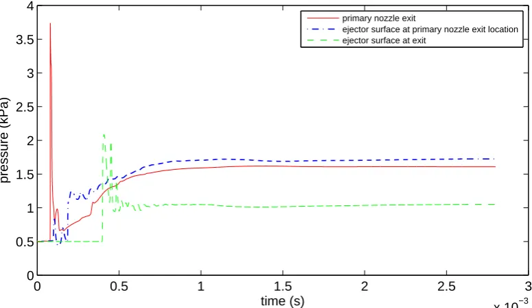
6.5 Temporal variation of static pressure during the simulations: primary nozzle exit, ejector surface at primary nozzle exit location, and ejector surface at exit. . . 102
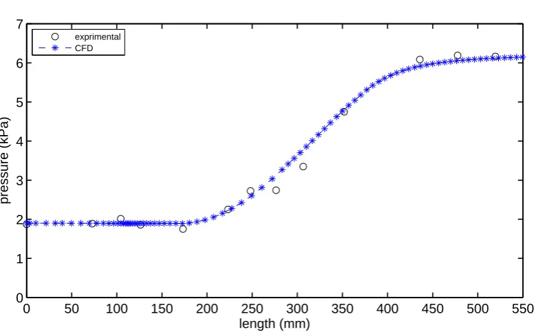
6.6 Comparison between Eilmer3 and experimental results of static pressure along the ejector for primary stream conditions of 270 kPa, 130, with an evaporator temperature of 14, and a condenser pressure of 6.1 kPa. 104
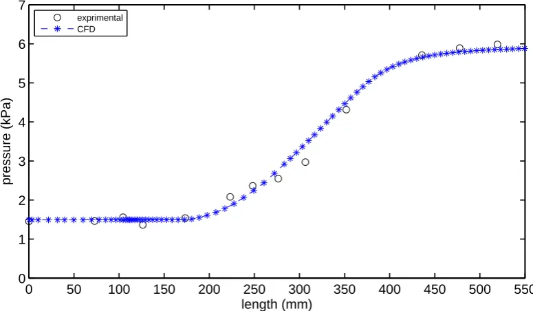
6.7 Comparison between Eilmer3 and experimental results of static pressure along the ejector for primary stream conditions of 270 kPa, 130, with an evaporator temperature of 10, and a condenser pressure of 6 kPa. . 105
6.8 Comparison between Eilmer3 and experimental results of static pressure along the ejector for primary stream conditions of 270 kPa, 130, with an evaporator temperature of 6, and a condenser pressure of 5 kPa. . 105
6.9 Comparison between Eilmer3 and experimental results of static pressure along the ejector for primary stream conditions of 200 kPa, 120, with an evaporator temperature of 14, and a condenser pressure of 5 kPa. . 106
6.10 Comparison between Eilmer3 and experimental results of static pressure along the ejector for primary stream conditions of 200 kPa, 120, with an evaporator temperature of 10, and a condenser pressure of 4.8 kPa. 106
6.11 Comparison between Eilmer3 and experimental results of static pressure along the ejector for primary stream conditions of 200 kPa, 120, with an evaporator temperature of 6, and a condenser pressure of 4.8 kPa. 107
6.12 Comparison between Eilmer3 simulations and experimental results for the entrainment ratio at primary stream conditions of 270 kPa, 130with an evaporator temperature of 14 and different condenser pressures. . 109
LIST OF FIGURES xxiii
6.14 Pressure map from Eilmer3 simulations at primary stream conditions of 270 kPa, 130 with an evaporator temperature of 14 and condenser pressure of 3.88 kPa. . . 111
6.15 Centreline pressure from Eilmer3 simulations at primary stream condi-tions of 270 kPa, 130 with an evaporator temperature of 14 and condenser pressure of 3.88 kPa. . . 111
6.16 Simulated velocity profiles for five sections along the ejector at primary stream conditions of 270 kPa, 130 with an evaporator temperature of 14 and condenser pressure of 3.88 kPa. AA-location is the separation flow at the wall of the diffuser. Each velocity increment corresponds to 100 m/s. . . 112
6.17 Velocity map from Eilmer3 simulation of the ejector at primary stream conditions of 270 kPa, 130with an evaporator temperature of 14and condenser pressure of 3.88 kPa. . . 112
6.18 Flow recirculation on the diffuser wall at section AA for conditions and location indicated in Figure 6.17. . . 112
6.19 Pressure map from Eilmer3 simulations at primary stream conditions of 270 kPa, 130 with an evaporator temperature of 14 and condenser pressure of 5.88 kPa. . . 113
6.20 Centreline pressure from Eilmer3 simulations at primary stream condi-tions of 270 kPa, 130 with an evaporator temperature of 14 and condenser pressure of 5.88 kPa. . . 113
xxiv LIST OF FIGURES
6.22 Velocity map from Eilmer3 simulation of the ejector at primary stream conditions of 270 kPa, 130with an evaporator temperature of 14and condenser pressure of 5.88 kPa. . . 114
6.23 Velocity map from Eilmer3 simulation of the secondary inlet at primary stream conditions of 270 kPa, 130with an evaporator temperature of 14 and condenser pressure of 5.88 kPa. . . 115
6.24 Pressure map from Eilmer3 simulations at primary stream conditions of 270 kPa, 130 with an evaporator temperature of 14 and condenser pressure of 6.5 kPa. . . 116
6.25 Centreline pressure from Eilmer3 simulations at primary stream condi-tions of 270 kPa, 130 with an evaporator temperature of 14 and condenser pressure of 6.5 kPa. . . 116
6.26 Simulated velocity profiles for five sections along the ejector at primary stream conditions of 270 kPa, 130 with an evaporator temperature of 14 and condenser pressure of 6.5 kPa. CC-location is the separa-tion flow at the wall of the mixing chamber. Each velocity increment corresponds to 100 m/s. . . 116
6.27 Velocity map from Eilmer3 simulation of the ejector at primary stream conditions of 270 kPa, 130with an evaporator temperature of 14and condenser pressure of 6.5 kPa. . . 117
6.28 Flow recirculation on the mixing chamber wall at section CC for condi-tions and location indicated in Figure 6.27. . . 117
LIST OF FIGURES xxv
6.30 Centreline pressure Eilmer3 simulated at primary stream conditions of 270 kPa, 130 with an evaporator temperature of 14 and condenser pressure of 6.9 kPa reverse flow . . . 119
6.31 Simulated velocity profiles for five sections along the ejector at primary stream conditions of 270 kPa, 130 with an evaporator temperature of 14 and condenser pressure of 6.9 kPa. DD and EE locations are the reverse flow at the secondary inlet region. Each velocity increment corresponds to 100 m/s. . . 119
6.32 Velocity map from Eilmer3 simulation of the ejector at primary stream conditions of 270 kPa, 130with an evaporator temperature of 14and condenser pressure of 6.9 kPa. . . 120
6.33 Reversed flow profile of section DD at secondary inlet region for condi-tions and location indicated in Figure 6.32. . . 120
6.34 Reversed flow profile of section EE at the conical mixing chamber for conditions and location indicated in Figure 6.32. . . 120
7.1 Photograph of the steam ejector system with mixing chamber. . . 123
7.2 Schematic diagram showing the mixing chamber. . . 124
7.3 Schematic diagram showing the mixing chamber at cross section AA. . 125
7.4 Photograph of the mixing chamber with windows, nozzle, pitot tube and bell mouth. . . 125
7.5 Overall arrangement of traverse mechanism. . . 126
7.6 Arrangement of the sliding support detail CC. . . 127
7.7 Primary stream stagnation pressure change during a period of 10 s. . . 129
xxvi LIST OF FIGURES
7.9 Mixing chamber static pressure change during the period of 10 s identi-fied in Figure 7.7. . . 129
7.10 Normalised pitot pressure from a point 3.5 mm below the centreline of the nozzle to a location 5 mm above the nozzle lip at 1 mm downstream from the nozzle lip, at a primary stream stagnation pressure of 270 kPa and temperature of 144. . . 130
7.11 Normalised pitot pressure at 1 mm distance from nozzle lip at a primary stream stagnation pressure of 270 kPa and temperature of 144. . . . 131
7.12 Normalised pitot pressure at 25 mm distance from nozzle lip at a primary stream stagnation pressure of 270 kPa and temperature of 144. . . 131
7.13 Normalised pitot pressure at 50 mm distance from nozzle lip at a primary stream stagnation pressure of 270 kPa and temperature of 144. . . 132
7.14 Normalised pitot pressure at 70 mm distance from nozzle lip at a primary stream stagnation pressure of 270 kPa and temperature of 144. . . . 132
7.15 Structure of the flow near the nozzle exit of over-expanded convergent-divergent nozzle (Oosthuizen and Carscallen, 1997). . . 133
7.16 Normalized pitot pressure data for four positions 1, 25, 50, and 70 mm downstream of the nozzle at 270 kPa stagnation pressure, 144 stag-nation temperature and 3 kPa back pressure. Each horizontal increment corresponds to 0.01. . . 135
7.17 Normalized pitot pressure data for four positions 1, 25, 50, and 70 mm downstream of the nozzle at 300 kPa stagnation pressure, 144 stag-nation temperature and 3 kPa back pressure. Each horizontal increment corresponds to 0.01. . . 135
LIST OF FIGURES xxvii
7.19 Estimation of the shear layer thickness at 25 mm downstream from the nozzle exit for the primary stream pressure of 270 kPa and 3 kPa back pressure. . . 136
7.20 Estimation of the shear layer thickness at 50 mm downstream from the nozzle exit for the primary stream pressure of 270 kPa and 3 kPa back pressure. . . 137
7.21 Estimation of the shear layer thickness at 70 mm downstream from the nozzle exit for the primary stream pressure of 270 kPa and 3 kPa back pressure. . . 137
7.22 Shape of jet flow interpreted from the pitot pressure data. . . 138
7.23 Geometry of the axisymmetric nozzle and mixing chamber with arrange-ment of blocks (denoted B0 to B8). . . 139
7.24 Geometry of the axisymmetric nozzle and mixing chamber with arrange-ment of blocks including blocks at the outlet which are used to control the back pressure (denoted B9 to B11). . . 139
7.25 Mesh used to simulate the free jet inside the mixing chamber. . . 140
7.26 Comparison of measured and simulated pitot pressure ratio profile across the steam jet at 1 mm distance from nozzle lip at 270 kPa stagnation pressure and 3 kPa back pressure. . . 141
7.27 Comparison of measured and simulated Mach number across the steam jet at 1 mm distance from nozzle lip at 270 kPa stagnation pressure and 3 kPa back pressure. . . 142
7.28 Map of simulated static pressures near the nozzle exit. . . 142
xxviii LIST OF FIGURES
7.30 Comparison of measured and simulated pitot pressure ratio profile across the steam jet at 25 mm distance from nozzle lip at 270 kPa stagnation pressure and 3 kPa back pressure. . . 143
7.31 Comparison of measured and simulated pitot pressure ratio profile across the steam jet at 50 mm distance from nozzle lip at 270 kPa stagnation pressure and 3 kPa back pressure. . . 144
7.32 Comparison of measured and simulated pitot pressure ratio profile across the steam jet at 70 mm distance from nozzle lip at 270 kPa stagnation pressure and 3 kPa back pressure. . . 144
7.33 (a) Illustration of the nozzle and mixing chamber arrangement including the control volume used in the analysis; (b) Illustration of pressure forces applied tho the control volume. . . 147
7.34 Mach number distributions at x = 70 mm deduced from the pitot pres-sure meapres-surement using an ideal gas assumption. . . 148
7.35 Momentum flux distributions at x = 70 mm deduced from the pitot pressure measurement using an ideal gas assumption. . . 148
8.1 Cross section of lenses separate to the pipe: two lenses with one pipe. . 151
8.2 Cross section of lenses as integral to the pipe. . . 151
8.3 Ray-tracing method for two of the optical arrangements: (a) Ordinary pipe with two lenses; (b) Pipe with integral lenses. . . 152
8.4 Photograph of the parallel section of the mixing chamber (integral lens) showing visualisation across the full height of the circular duct. . . 153
8.5 Arrangement of Toepler’s schileren method (Schardin, 1947). . . 154
LIST OF FIGURES xxix
8.7 Camera, 600 mm focal lens, and knife edge mounted on slide rail with camera monitor. . . 157
8.8 Lamp, filter, condenser lens, slit, and 1000 mm focal lens mounted on slide rail with Schileren object. . . 157
8.9 Schlieren image of air discharged from the nozzle within the mixing chamber for stagnation conditions of 380 kPa and 25. . . 158
8.10 Schlieren image of air discharged from the nozzle within the mixing chamber for stagnation conditions of 380 kPa and 25 with a pitot tube positioned close to the nozzle exit. . . 159
8.11 (a) Schlieren image of the steam nozzle within the mixing chamber for stagnation conditions of 380 kPa and 144, with mixing chamber pres-sure of 3 kPa; (b) Same photograph as part (a) but annotated showing the analysis zone and the observed edge effect. . . 160
8.12 Normalized brightness of the Schlieren image within the analysis zone (defined in Figure 8.11(b)) for steam flow at stagnation conditions of 380 kPa and 144 with a mixing chamber static pressure of 3 kPa. . . . 161
8.13 Density map of steam at stagnation conditions of 380 kPa and 144 with a back pressure of 3 kPa. . . 163
8.14 Density map of air at stagnation conditions of 380 kPa and 25 with a back pressure of 3 kPa. . . 163
8.15 Photograph showing ice forming inside the mixing chamber. Primary stream operating conditions were 270 kPa and 144. . . 164
8.16 Photograph showing cracks in the mixing chamber. . . 165
A.1 Primary nozzle, all dimensions in mm. . . 181
xxx LIST OF FIGURES
A.3 Nozzle holder, all dimensions in mm. . . 182
A.4 Plenum chamber, all dimensions in mm. . . 183
A.5 Secondary inlet, all dimensions in mm. . . 184
A.6 Mixing chamber with parallel section, all dimensions in mm. . . 185
A.7 Diffuser dimensions with pressure transducers holes, all dimensions in mm. . . 186
A.8 Steam generator and stirrer, all dimensions in mm. . . 187
A.9 Evaporator details, all dimensions in mm. . . 188
A.10 (a) Single phase half controlled rectifier; (b) Evaporator element heater. 189
A.11 Condenser details, all dimension in mm. . . 190
A.12 (a) Front panel with switches and temperature controller; (b) Internal side of enclosure. . . 192
A.13 Diagram of the control circuit. . . 193
A.14 Drawing of the power circuit. . . 193
B.1 Evaporator chamber. . . 199
B.2 Evaporator chamber. . . 200
B.3 Evaporator chamber. . . 200
B.4 Evaporator chamber. . . 201
B.5 Illustrates filling evaporator with water . . . 202
LIST OF FIGURES xxxi
C.1 Photograph of the pneumatic dead-weight tester model 550 series (Bu-denberg). . . 205
C.2 Photograph of the hydraulic dead-weight tester model 580 series (Bu-denberg). . . 205
C.3 Calibration of the Kulite pressure transducer - representative result. . . 206
C.4 Calibration of the Wika low pressure range transducer - representative result. . . 206
C.5 Calibration ofthe Wika high pressure range transducer - representative results. . . 207
C.6 Calibration of thermocouple - representative result. . . 209
C.7 Dosing pump with suction hose from beaker. . . 210
C.8 Calibration LCD display for calibration on dosing pump. . . 210
C.9 Factory calibration in LCD display. . . 211
C.10 Actual dosed volume in LCD display. . . 211
D.1 Light ray passing through perspex tube and perspex lens. . . 213
D.2 Light ray passing through perspex tube and perspex lens: for calculation of the coordinates of the lens. . . 215
D.3 (a) Photograph of the separate pipe with two lenses; (b) Photograph of the separate pipe with two lenses showing visualisation across the full hight of the pipe. . . 216
D.4 Light ray passing through the integral lens: definition angles. . . 217
xxxii LIST OF FIGURES
List of Tables
3.1 Features for both steam generator options. . . 42
3.2 Specifications of pressure transducers (Wika, 2011; Kulite, 2011). . . 49
4.1 Comparison of primary mass flow rate measurement by two methods. . 55
4.2 Comparison of secondary mass flow rate measurement by two methods. 56
4.3 Estimates of non-electrical heat gain by the evaporator. . . 59
4.4 Variation of COP with evaporator load for NXP = -32 mm. . . 63
4.5 Variation of primary stream stagnation pressure during the test time. . 67
4.6 Variation of primary stream stagnation temperature during the test time. . . 67
4.7 Variation of evaporator pressure for different loads during the test time as indicated in Figure 4.6(a). . . 67
4.8 Variation of evaporator temperature for different loads during the test time as indicated in Figure 4.6(b). . . 67
4.9 Variation of condenser pressure during the test time. . . 67
xxxiv LIST OF TABLES
5.1 Secondary and primary stream mass flow rates for three different pri-mary stream temperatures with an evaporator temperature of 14. . . 81
6.1 Different grids used in the simulations. . . 96
6.2 Ejector operation conditions specified in the simulations. . . 98
6.3 Number of cells in the axial and radial directions for coarse, medium, and fine resolution cases. . . 100
6.4 Comparison of different turbulence models with Eilmer3 simulation. . . 107
7.1 Ejector operating conditions used in the simulation. . . 139
C.1 Calibration of Kulite and Wika pressure transducers. Vmeas= measured
Notation
Roman symbols
a Sonic speed, m/s
A Area, m2
AT Nozzle area ratio
C1 Molecular weight correction factor C2 Temperature correction factor Cd Discharge coefficient nozzle
Cp Specific heat capacity at constant pressure, kJ/kg K
Cv Velocity coefficient
d Inside diameter of stainless steel pipe, m d∗ Diameter of throat nozzle area, m D Diameter of throat ejector, m Di Inside diameter of copper tube, m Do Outside diameter of copper tube, m f Internal roughness for stainless steel, m h4,5,6,9,.. Enthalpy, kJ/kg
H Height of the evaporator, m
hi inside tube heat transfer coefficient, W/m2K
ho Outside tube heat transfer coefficient, W/m2K
hf Head losses, m
Iturb Turbulence intensity
xxxvi notation
k Thermal conductivity, W/m K
L Length, m
Lm Conical mixing chamber length, m
Ln Secondary inlet length, m
Lp Parallel mixing chamber length, m
Ld Diffuser length, m
M Mach number
˙
mp Primary mass flow rate, kg/hr
˙
ms Secondary mass flow rate, kg/hr
Np Primary ratio
Ns Compression ratio
N u Nusselt number P Pressure, kPa
Pc Condenser pressure, kPa
Pco Breakdown pressure, kPa
Pb Background pressure, kPa
Pe Nozzle exit pressure, kPa
Ppit Pitot tube pressure, kPa
P r Prandtl number Qe Cooling load, W
Qee Power input to the evaporator element heater, W
Qg Input heat to the steam generator, W
q Heat transfer from oil to water, W R Gas constant, kJ/kg K
R1,2,3, ... Heat resistance K/W
r1,2,3, ... Radius of pipe and insulation, m
T Temperature,
Ts Surface temperature,
Tf Fluid temperature,
u Velocity, m/s
V Velocity of steam inside the pipe, m/s
W Watt
NOTATION xxxvii
W m Watt meter,
y Distance, mm
y+ Dimensionless wall distance
Greek symbols
ω Entrainment ratio ρ Density, kg/m3 ρwall Wall density, kg/m3
θm Mixing chamber angle
θd Diffuser angle
γ Specific heat ratio
ηN Nozzle’s isentropic efficiency
τwall Wall shear stress, kg/m s2
µ Dynamic viscosity, Pa.s µwall Wall dynamic viscosity, Pa.s
β Volumetric thermal expansion coefficient, 1/K ν Kinematic viscosity, m2/s
µlam Laminar viscosity, m2/s
µturb Turbulent viscosity, m2/s
xxxviii notation
Subscripts
o Stagnation condition i Inside
c Cold
h Hot
Superscripts
∗ Critical
Acronyms & Abbreviations
ASHRAE American Society of Heating, Refrigerating and Air-Conditioning En-gineers, Inc.
CFD Computational fluid dynamics CMA Constant mixing area
CPM Constant pressure mixing C.P. Critical condenser pressure
COP Coefficient of performance of cycle CV Control volume
ESDU Engineering sciences data unit I.P. Intersect point
LMTD Log mean temperature difference NXP Nozzle exit position
Chapter 1
Introduction
1.1
Applications of an ejector
Ejector or jet pumps are used extensively in the power generation, nuclear and chemical processing industries. Ejectors also have applications in distillation, vacuum evapora-toration and drying (for instance, soap drying). Ejectors have many advantages over conventional pumps or compressors such as extremely reliable and stable operation, the absence of moving parts, and the ability to handle highly corrosive vapours and fluids. Ejectors can be fabricated in wide range of sizes and can operate safely under hazardous conditions (ESDU86030, 1986).
Ejectors have a very low efficiency compared with normal pumping system but when a source of low grade or waste energy is available, an ejector may be cheaper to operate than a mechanical pump (Dandachi, 1990). Recently, ejectors have become of interest for researchers in air conditioning and refrigeration fields.
1.2
Ejector refrigeration systems
hydrochloroflu-2 Introduction
orocarbons (HCFC) (e.g. R-22 and R-123) and hydrofluorocarbons (HFC) (e.g. R-32 and R-134a) (ASHRAE, 2002). These working fluids can cause serious problems like depletion of the stratospheric ozone layer, production of large amounts of greenhouse gas emissions and global warming. Furthermore, refrigeration and air conditioning systems are normally driven by electricity, which strongly increases the demand for electricity and the consumption of fossil fuel. An alternative solution for this problem is the application of low-grade waste energy or solar energy. There are a number of types of air conditioning systems potentially powered by such energy including ab-sorption, adsorption and desiccant coolers. However, these systems are typically large and expensive. Evaporative coolers are another possibility but these have a high level of water consumption and may not be effective at all locations. Ejectors can also be driven by waste-energy or solar power and through an increasing use of waste or solar energy in refrigeration systems, the relative demand for electrical energy sources can be decreased.
Figure 1.1 illustrates an ejector refrigeration cycle. The ejector provides the compres-sion effect for the cycle.
1.3
Ejector operation
1.3 Ejector operation 3
heat absorbed from cold space pump 4 evaporator condenser generator 9 6 7 2 8 ejector heat rejected to atmosphere expansion device
heat added from solar or waste source
or
.
(a)
.
[image:45.595.208.429.84.671.2](b)
Figure 1.1: (a) Ejector pump refrigeration system; (b) Illustrative p-h diagram of a closed
4 Introduction
diffuser. Finally, the mixture leaves the diffuser to enter the condenser at position C. An important parameter in ejector design is the entrainment ratio which is defined as ω= ( ˙ms/m˙p), where ˙ms is the secondary mass flow rate and ˙mp is the primary mass
flow rate.
Figure 1.2: Geometry of an ejector.
Ejector refrigeration systems are promising because of their relative simplicity and low capital cost and the fact that the system can be powered by “low grade” energy (for example solar energy) instead of electricity. This means ejector-based refrigeration systems potentially have significant environmental benefits, especially when a renew-able energy source such as solar energy can be used. The primary disadvantage with ejector-based refrigeration systems is the low coefficient of performance (COP). As illustrated in Figures 1.1(a) and 1.1(b), the refrigeration effect is ˙ms(h6−h9) and the
power supply (heat supply) is ˙mp(h4−h2). The COP is defined to be COP = refrigeration effect
(power supply + pump work) (1.1)
and when the pump work is very small compared with the power supply (which is usually the case), the pump work can be neglected and the COP can be approximated as
COP = m˙s(h6−h9)
˙
mp(h4−h2)
(1.2)
COP = ω(h6−h9)
(h4−h2)
(1.3)
Clearly the entrainment ratioω = ( ˙ms/m˙p) is directly proportional to the COP,
1.4 Ejector design 5
1.4
Ejector design
Supersonic ejector design profoundly affects refrigeration system performance. Previ-ous studies have presented varying degrees of success when attempting to computation-ally simulate and model the static pressure distributions within the mixing region of ejectors. Ejector design optimisation based on computational simulation or modelling is not yet a reliable strategy because of the variable performance of computational tools. The modest degree of success achieved so far with ejector computational sim-ulation arises because of the complexity of the ejector flows which typically include strong turbulent mixing, high speed compressible vapour, strong pressure gradients and shock waves. To clarify the mixing and compression processes occurring in ejectors, additional experimental data are required for validation of thermodynamic modelling and numerical simulations.
1.5
Objectives of the dissertation
The present work targets the generation and interpretation of new data on the mixing and compression processes in a representative ejector apparatus. Steam is used as the working fluid because of its well-established thermodynamic and transport properties combined with its ease of handling in the laboratory environment. The main objectives of this study are to:
1. Design and commission an open steam ejector refrigerant cycle with a cooling capacity sufficient for visualisation purposes.
2. Confirm system performance over an appropriate range of operating conditions.
3. Design and commission a transparent mixing chamber suitable for visualisation of ejector flows.
4. Acquire new data which provides additional insight into the ejector mixing and compression processes.
6 Introduction
1.6
Overview of the Dissertation
This dissertation is organised as described in the following sections.
1.6.1 Chapter 2 Literature review
The literature review is presented in three main sections. The first section presents an overview of ejector design and operation, while section 2 presents an overview of ex-perimental flow visualisation studies and section 3 discusses computational simulation results obtained for different ejector configurations.
1.6.2 Chapter 3 Overview of the design of the apparatus
This chapter presents the design of the steam ejector refrigeration apparatus and the measurement methods used to characterize the coefficient of performance of the system. A new design for the steam generator is introduced and is compared with a conventional boiler. To weigh the amount of water induced from the evaporator during test time, a new evaporator chamber is also introduced.
1.6.3 Chapter 4 System performance
Standard operating conditions for the ejector apparatus were established during com-missioning of the rig. Methods and results for the calculation of COP, heat losses from the primary stream, and the heat gain by the evaporator from non-electrical sources are also presented. Measurement methods and results for the mass flow rates of the primary and secondary flows and the critical condenser pressure are also presented.
1.6.4 Chapter 5 Ejector results and discussion
1.6 Overview of the Dissertation 7
pressure on pressure distributions in the mixing chamber and diffuser, and the effect of evaporator load on the performance of the apparatus. Comparison of the present experimental results with previous work is also presented.
1.6.5 Chapter 6 Computational simulation
Computational Fluid Dynamics (CFD) simulation of the ejector was also performed using a k-ω turbulence model and good agreement between the experimental data and the simulations for wall static pressure was achieved. Pressure and velocity maps identifying some features such as recirculation flow within the diffuser and mixing chamber, and reverse flow in the secondary inlet are also discussed.
1.6.6 Chapter 7 Mach 4 steam jet
A new method to characterise the steam flow in the mixing chamber was required. For this task, a special pitot tube apparatus was designed and fabricated. Pitot pressure measurements were performed with the pitot probe positioned at four locations from the lip of the nozzle: 1, 25, 50, and 70 mm. The experimental results were analysed with the aid of CFD simulations and a momentum integral analysis.
1.6.7 Chapter 8 Flow visualisation
8 Introduction
1.6.8 Chapter 9 Conclusions and future work
Chapter 2
Literature review
2.1
Introduction
There are several ongoing attempts to investigate the low coefficient performance of ejectors compared to conventional pumping systems. Most efforts have adopted exper-imental and computational approaches, although analytical work has played a signifi-cant role in the development of ejector design approaches.
2.2
Ejector performance studies
2.2.1 Analytical work
10 Literature review
a better coefficient of performance. One-dimensional constant area flow models have been used to solve many supersonic ejector optimisation problems. The Mach number for the primary nozzle and the ejector area ratio were found to have a significant influence on performance parameters such as the compression ratio or the entrainment ratio (Dutton and Carroll, 1986).
Huang et al. (1999) carried out a one-dimensional ejector performance analysis for ejec-tor operation. Referring to Figure 2.1, a number of assumptions were made including:
A hypothetical throat occurs inside the constant-area section of the ejector cross section y-y, meaning the entrained flow reaches a choked condition at the y-y section.
Primary and secondary flows start mixing at the hypothetical throat with a
constant pressure.
A shock will appear at cross section s-s, causing a sharp pressure rise.
Huang et al. (1999) studied 11 ejectors with R141b as the working fluid. The experi-mental results were used to calculate the coefficients of the primary nozzle and other parameters defined in the one-dimensional model. It was shown that the analytical investigation can accurately predict the performance of the ejectors but the modelling assumptions would not be applicable to all ejector configurations.
2.2 Ejector performance studies 11
Al-Ansary (2004) formulated a one-dimensional model of two phase flow in ejectors. The effect of adding a non-volatile liquid to the primary stream in an ejector was evaluated. A control volume analysis was used to develop a model based on a number of reasonable assumptions, such as:
The volatile fluid is an ideal gas.
The velocities of primary and secondary streams at the inlet are negligible.
The size of the droplets of the non-volatile fluid is very small such that the two components have the same velocity and temperature at any given position. This means the flow is homogeneous at the exit.
The ejector is adiabatic and all properties of the fluids are constant.
The following results were deduced from the analysis.
A normal shock wave leads to compression of the mixture of primary and
sec-ondary flows at the end of the mixing section.
The adding of a non-volatile liquid to the primary stream causes a slight decrease
to the flow rate of gaseous components.
The choking phenomenon is a function of the value of the entrainment ratio.
The entrainment ratio is increased through adding a non-volatile liquid to the primary flow.
Pridasawas (2006) discussed the effect of the back pressure, also called the condenser pressure Pc, on the entrainment ratio. Three ejector operation regimes are associated
with the condenser pressure, see Figure 2.2.
12 Literature review
The COP decreases when the condenser pressure is higher than the critical
pres-sure. In this case, choking occurs only in the primary flow, not in the secondary flow. Therefore, the entrainment ratio decreases with increase Pc.
The COP drops to zero when the condenser pressure is higher than the limiting
pressure of the ejector, Pco. In this case, back-flow occurs in the secondary flow.
In Pridasawas (2006), many governing equations were used during the theoretical anal-ysis, which adopted a number of assumptions such as the process in the ejector being adiabatic. Mixing and friction loss were calculated in the form of an isentropic ef-ficiency. Furthermore, the refrigerant was assumed to have constant properties and steady flow along the ejector was also assumed.
Figure 2.2: Schematic illustration of operation regimes associated with the condenser
pressure (Pridasawas, 2006).
2.2.2 Operating conditions
2.2 Ejector performance studies 13
Meyer, Harms and Dobson (2009) also examined a steam ejector which was setup in an open system configuration. The tests included a boiler temperature range between 85 and 140, an evaporator temperature range from 5to 10, and a maximum condenser pressure of 5.63 kPa. The primary nozzle throat diameters used were 2.5, 3, and 3.5 mm. The results reveal that the steam ejector system can be operated at boiler temperatures below 100. Meyer et al. (2009) concluded that the key parameters that govern the functioning of the steam ejector are the evaporator temperature, boiler temperature, condenser pressure, and primary nozzle exit position.
Chunnanond and Aphornratana (2004) performed experiments using a closed steam ejector refrigeration system. The experiments were conducted over a boiler tempera-ture range from 120 to 140, an evaporator temperature range from 5 to 15, and with three primary nozzle throat diameters: 2, 1.75, and 0.5 mm. From their re-sults, it appears that the superheating of the primary flow does not have an impact on either the COP of the steam ejector or the critical condenser pressure. Furthermore, the results show that the COP of the system decreased when the primary pressure was increased at constant evaporator temperature.
2.2.3 Primary nozzle arrangement
Chang and Chen (2000) found that the performance of the ejector using a petal nozzle was better than ejector performance with a conical nozzle for large nozzle area ratios. Figure 2.3 illustrates the conical and petal nozzles. Both nozzles have the same throat and exit areas of 3.14 and 63.4 mm2, respectively. The exit plane of the petal nozzle was formed by six lobes. The experiments were carried out at various evaporator temperatures, boiler temperatures, and condenser pressures. The results reveal that the entrainment ratio and compression ratio can be improved if the petal nozzle with large area ratio is used in the steam ejector.
14 Literature review
Figure 2.3: Primary nozzle geometries used by Chang and Chen (2000).
demonstrate that the cooling capacity decreased when the spindle moved toward the nozzle because of the decrease in primary flow rate. The critical back pressure rose with the increase in the spindle position. The COP and cooling capacity increased with evaporator temperature. The maximum boiler temperature was less than 95 and the optimum COP and entrainment ratio were found at a boiler temperature of about 90.
2.3 Flow visualisation studies 15
2.3
Flow visualisation studies
Throughout history, experimental flow visualisation has been an important instrument in fluid dynamics research and remains a very helpful tool for the understanding of complex flow phenomena and the validation of analytical and computational models. Up to this point, little work has been done in the area of flow visualisation within ejectors.
Fabri and Siestrunck (1958) utilised schlieren methods to visualise the flow in six noz-zles for supersonic air ejectors operated over various ranges of pressure. Experimental results were compared with theoretical work and a number of the flow regimes were categorised. Matsuo, Sasaguchi, Tasaki and Mochizuki (1981) used schlieren methods to analyse the performance of a supersonic flow of air through a rectangular ejector without a secondary flow. Ejector operation with an exhaust or vacuum pump was investigated.
Hong, Alhussan, Zhang and Garris (2004) used a schlieren system and a high speed camera to investigate a new idea to improve the efficiency of the ejector by reducing the velocity of the primary flow by allowing it to expand through a rotor-vane. Schlieren visualisation was used to capture unsteady phenomena in the entrance region of the mixing chamber. Optical measurements using schlieren were more sensitive to changes of density perpendicular to the flow than in any other direction (Dvorak and Safarik, 2005). However, the shadowgraph and schlieren methods do not allow visual distinction between two interacting (primary and secondary) streams in an ejector (Bouhanguel et al., 2010).
16 Literature review
used in qualitative studies when water nanodroplets were formed in an induced ejec-tor (Desevaux, 2001a). For this purpose a TSI atomiser (model 9306A) was used to produce fluorescent doped droplets of diameter 0.1-2 µm. Figure 2.5 shows the experimental rig including a TSI atomiser and the data acquisition system used by Desevaux (2001b).D Desevaux (2001b) continued investigating the formation of water
Figure 2.5: Optical device, TSI atomiser and acquisition system used by Desevaux (2001b).
nanodroplets in an induced air ejector. The water nanodroplets occurred when the induced air was moist. An analysis of the light scattered by the droplets generated by condensation within the flow revealed that their mean diameter did not exceed 0.1µm.
Desevaux and de Sousa (2004) conducted a visualised air flow experiment inside a supersonic ejector. The laser tomography visualisation was compared with a compu-tational fluid dynamic (CFD) simulation. Zero secondary flow and free entrainment of induced air were examined through visualisation.
Marynowski et al. (2009) presented visualisation results for droplet condensation with moist air supplied to the ejector. The results were compared with visualisation from CFD. Figure 2.6 illustrates reasonable agreement between experimental visualisation and CFD simulations for three values of primary stagnation pressureP1 with the free
2.3 Flow visualisation studies 17
(Marynowski et al., 2009).
Figure 2.6: Comparison between experimental visualisation and numerical CFD
visualisa-tion (Marynowski et al., 2009).
Rayleigh scattering and Mie scattering techniques were improved by Bouhanguel et al. (2010) to visualise supersonic air flow inside the ejector. Figure 2.7 illustrates the experimental arrangement using a laser beam from a CW argon laser with 120 mW of power in the green line (λo=514 nm) as a light source. The camera had 500x582
18 Literature review
Figure 2.7: Experimental rig used by Bouhanguel et al. (2010).
2.4
Computational fluid dynamics simulations
Computational fluid dynamics (CFD) was used by Riffat, Gan and Smith (1996) to simulate ejector performance. A commercial CFD software package was used to anal-yse ejector performance with different types of refrigerant and various geometries for the primary nozzle. However, Riffat et al. (1996) modelled the refrigerant as an in-compressible flow to avoid a convergence difficulty with the computational method. Clearly this is an invalid assumption in the context of supersonic ejector design.
2.4 Computational fluid dynamics simulations 19
the experimental results indicated the presence of a shock.
Computational fluid dynamic simulations were used by Rusly (2004) to simulate and design an ejector working with R141b. Simulations included three different flow fields related to operating conditions and the ejector entrainment ratio. The best perfor-mance of the ejector was achieved when operating in an over expanded state and the entrained flow was choked. However, a weak oblique shock wave was observed in the ejector simulations, especially in the constant area section filling the centre part of the tube slightly off the wall.
Bartosiewicz, Aidoun, Desevaux and Mercadier (2005) studied the performance of six well-known turbulence models, applied to supersonic air ejectors using CFD simula-tions. The shock strength, shock location and the average pressure recovery were the focus of the simulations. Supporting experiments were also performed and centreline pressure was measured throughout the ejector using a capillary probe. The results were compared with the measurements of Desevaux and Aeschbacher (2002). The best model was the k-ω-SST model which demonstrated the best performance in stream mixing. In addition, the CFD simulations showed some ability to simulate the differ-ent operational modes of a supersonic ejector, ranging from the on-design point, with maximum flow rate (choking), to off-design, in which the secondary flow rate drops to zero (complete malfunctioning).
Normally, ejectors are classified as either constant mixing area (CMA) ejectors or con-stant pressure mixing (CPM) ejectors, as illustrated in Figure 2.8. The flow phenomena and performance of both types have been assessed using the CFD code FLUENT, op-erated with thek-turbulence model, and an ideal gas as the working fluid (Pianthong et al., 2007)
20 Literature review
Figure 2.8: Two ejector types: (a) constant pressure mixing ejector (b) constant mixing
area ejector (Pianthong et al., 2007).
change with back pressure. The operation of an ejector can be classified into three regions as show in Figure 2.10: choked flow, unchoked flow and reversed flow. Despite increasing the back pressure, points A, B and C in the ejector still operated within the choked regime because the back pressure did not exceed the critical point value. Points D and E were unchoked and reversed flow respectively because the downstream pressure was increased more than the critical value.
Figure 2.9: Variation of calculated entrainment ratio of a steam ejector: effect of operating
2.4 Computational fluid dynamics simulations 21
Figure 2.10: Filled contours of Mach number: effect of downstream pressure. All operating
points A, B, C, D and E correspond to those shown in Figure (2.9) (Sriveerakul et al.,
2007b).
Hemidi et al. (2008) presented comparisons between CFD and experimental measure-ments. A wide range of pressure operating conditions was tested and they focused on the different behaviour of two turbulence models: k- and k-ω-SST. Figure 2.11 illustrates the differences between the two turbulence models, and how results vary depending on the primary pressure. The difference between the two models became very small when the primary pressure was increased. In contrast to the work of Bar-tosiewicz et al. (2005), good validation outcomes were obtained for the supersonic air ejector using the k- model for both on-design and off-design conditions: Figure 2.11(b). The k-ω-SST model gave similar results to the k- model for the on-design conditions but over predicted the results at off-design conditions as shown in Figure 2.11(a) where the entrainment ratio was very low. Simulation at off-design conditions appears more sensitive to condenser pressure Pc.
22 Literature review
c
Pc
sfsrf
c c
Figure 2.11: Comparison between two turbulence models, k- and k-ω-SST, and
exper-imental data on the entrainment ratio at different primary stream pressures: (a) Po
1 =
3 bar, (b)Po
1 = 6 bar (Hemidi et al., 2008).
the secondary flow near to the primary nozzle exit with different condenser pressure Pcat off-design operation for the case ofP1 = 6 bar, and a secondary pressure of 1 bar.
As the condenser pressure was increased, a flow detachment occurred close to the wall of the mixing chamber for thek-simulation. When the condenser pressure was fur-ther increased, this detachment became a large recirculation zone for Pc = 1.25 bar.
When Pc reached 1.3 bar, the recirculation claimed the majority of the area and the
2.4 Computational fluid dynamics simulations 23
Figure 2.12: Comparison between two turbulence models k- andk-ω-SST. Contours of
the stream function for the top half of the mixing chamber (Hemidi et al., 2009).
The performance of a steam ejector was simulated using thek-turbulence model by Varga, Oliveira and Diaconu (2009). The different ejector efficiencies (nozzle, suction, mixing and diffuser) were examined. The results indicated that nozzle efficiency can be deemed independent of operating conditions, and that this efficiency was only slightly affected by nozzle diameter. Suction efficiency was considered constant before the back pressure reached the critical value, and the suction efficiency dropped when back pressure went beyond the critical value. Other efficiencies increased with increasing back pressure until the critical value was reached.
24 Literature review
pressure closer to the experimental results than the other two models tested. The CFD simulation results also demonstrate that the entrainment ratio and critical back pressure of the rectangular nozzle were 7.1 % and 21.3 % lower respectively than for the conical nozzle, and the entrainment ratio and critical back pressure of the elliptic nozzle were 7.9 % and 21.3 % lower respectively than the conical nozzle. Relative to the performance of the conical nozzle, the square nozzle enhanced the entrainment ratio by about 2 % and decreased the critical back pressure by about 2.1 % while the cross-shape nozzle improved the entrainment ratio by about 9.1 % and decreased the critical back pressure by about 6.4 %.
lengths to investigate the effect of geometry on ejector perfor-mance. In this paper, mixing chamber No.1 and throat No.3 were chosen and the primary nozzle exit position was placed at NXP of 35 mm, which implies it is placed into the mixing chamber. The
performance of the ejector with nozzle No.1[1]was chosen as the
baseline of the other four. The geometrical configurations of thefive
nozzles are shown inFig. 3and the parameters are listed inTable 1.
These nozzles only differ in the divergent part and have the same area ratio of the nozzle exit to the nozzle throat, which equals
to16.0. The nozzle exit diameter (D) is 8.0 mm. The area ratio of the
constant area throat (ejector throat) to that of the nozzle throat is
90.25. The length of the ejector throat equalsfive times its diameter
(19.0 mm). As shown inTable 1, the cross-shaped nozzle has the
greatest exit plane perimeter (EPP), 57.0% higher than that of the conical nozzle, due to its convoluted trailing edge. In this work, the
work conditions were saturated temperatureTpof primaryfluid of
130C, secondaryfluid saturated temperatureTsof 10C and back
pressurePcof 3e5.5 kPa.
The flow inside the ejector is assumed to be steady and
compressibleflow, controlled by the Reynolds averaging Navier
Stokes equations together with the continuity equation and the
energy equation. To the authors’ knowledge, three kinds of
k-epsilon turbulence models, namely the Standard, RNG and Real-izable k-epsilon model, have been frequently used to govern the
turbulence characteristics[1e6,9,12e16]. The realizable k-epsilon
Fig. 2.Performance characteristics of a steam ejector.
Fig. 3.Characteristic nozzle dimensions in mm.
X. Yang et al. / International Journal of Thermal Sciences 56 (2012) 95e106 97