ADI method based on
C
2-continuous two-node integrated-RBF
elements for viscous flows
D.-A. An-Vo1, N. Mai-Duy1, C.-D. Tran1, T. Tran-Cong1,∗
∗Corresponding author. Tel.: +61 7 4631 1332; fax: +61 7 4631 2110
Email addresses: [email protected](D.-A. An-Vo),[email protected](N.
Mai-Duy),[email protected](C.-D. Tran),[email protected](T. Tran-Cong)
1
Abstract: We propose a C2-continuous alternating direction implicit (ADI) method for
the solution of the streamfunction-vorticity equations governing steady 2D incompressible viscous fluid flows. Discretisation is simply achieved with Cartesian grids. Local two-node integrated radial basis function elements (IRBFEs) [D.-A. An-Vo, N. Mai-Duy, T. Tran-Cong, A C2-continuous control-volume technique based on Cartesian grids and two-node
integrated-RBF elements for second-order elliptic problems, CMES: Computer Modeling in Engineering & Sciences 72 (2011) 299-334] are used for the discretisation of the diffusion terms, and then the convection terms are incorporated into system matrices by treating nodal derivatives as unknowns. ADI procedure is applied for the time integration. Following ADI fatorisation, the two-dimensional problem becomes a sequence of one-dimensional problems. The solution strategy consists of multiple use of a one-dimensional sparse matrix algorithm that helps saving the computational cost. High levels of accuracy and efficiency of the present methods are demonstrated with solutions of several benchmark problems defined on rectangular and non-rectangular domains.
Keywords: Navier-Stokes equations, integrated-radial-basis-function elements,C2-continuous
solutions, Cartesian grid, ADI method, local RBF approximation.
1. Introduction
The dimensionless Navier-Stokes (N-S) equations for steady incompressible planar viscous flows, subject to negligible body forces, can be expressed in terms of the streamfunction ψ
and the vorticity ω as follows.
∂2ψ ∂x2 +
∂2ψ
∂y2 +ω = 0, (1)
∂2ω ∂x2 +
∂2ω ∂y2 =Re
∂ψ
∂y ∂ω ∂x −
∂ψ ∂x
∂ω ∂y
, (x, y)T ∈Ω, (2)
where Re = UL/ν is the Reynolds number, in which L is the characteristic length, U the characteristic speed of the flow andν the kinematic viscosity of the fluid. The vorticity and streamfunction variables are defined by
ω= ∂v
∂x − ∂u
∂y, (3)
∂ψ ∂y =u,
∂ψ
whereu and v are the xand y components of the velocity vector. In this study, the method of modified dynamics or false transients (e.g. [1, 2]) is applied to obtain the structure of a steady flow. The governing equations (1) and (2) are modified as
∂2ψ ∂x2 +
∂2ψ
∂y2 +ω= 0, (5)
∂ω ∂t +
∂2ω ∂x2 +
∂2ω ∂y2 =Re
∂ψ
∂y ∂ω ∂x −
∂ψ ∂x
∂ω ∂y
. (6)
A steady state solution to (5) and (6), which is obtained by integrating the equations from a given initial condition up to the steady state, is also solution to (1) and (2).
Cartesian-grid-based methods for solving (1) and (2) can be very economical owing to the facts that (i) generating a grid is low-cost; and (ii) ADI procedure [3, 4] can be straightfor-wardly applied to accelerate computational processes. The approximations for the dependent variables and their spatial derivatives can be constructed globally on the whole grid or locally on small segments of the grid. A very prominent local approximation scheme is the finite-difference (FD) which can be based on two nodes (first-order accuracy) and three nodes. The three-node approximations can take the second-order central difference (CD) form, e.g. [5], or high-order compact (HOC) implicit forms, e.g. [6–8], where nodal values of the field variables and their derivatives are considered as unknowns. The three-node HOC implicit schemes can achieve higher order numerical accuracy and yield greater computational effi-ciency compared with CD schemes for the same level of the accuracy, e.g. [7]. However, the computational cost of these implicit schemes was quite high because of time consumption for solving (i) less-than-optimal banded matrices (block diagonal structure where each block corresponds to a grid line) [9–11]; or (ii) a larger number of equations per grid point [7], i.e. 3N equations for N grid points in 1D problems and 5N equations for N grid points in 2D problems. In addition, these finite difference schemes (i.e. the two-node and the three-node schemes) typically produce solutions which are continuous for the fields but not for their partial derivatives, i.e. C0-continuity. The grid thus needs to be sufficiently fine to mitigate
the effects of discontinuity of partial derivatives.
includes Nη equations (matrix dimensions are Nη ×Nη) for Nη grid points on a particular
η-grid line whereη representsxand y. These relatively small sets of equation (in tridiagonal matrix form) are solved separately and effectively by the Thomas algorithm that helps saving the computational cost. However, the numerical accuracy of PR-ADI is only second-order in space [3]. The combination of the ADI approach and the HOC schemes has been proposed by e.g. [7, 10] for solving fluid mechanics problems, by e.g. [12] for parabolic partial differential equations, and by e.g. [9, 11] for convection-diffusion problems. Hirsh [7] applied the ADI procedure to HOC implicit schemes for simulating a model square cavity flow through solving sets of 3Nη equations for Nη grid points on η-grid lines. Adam [12] further reduced the number of equations on each grid line to sets of 2Nη equations by means of the so-called implicit elimination. Recently, Karaa and Zhang [9] and Karaa [10] solve sets ofNη equations on η-grid lines through block matrices. However, as shown in [13], the solution quality of this ADI method is degraded for convection-diffusion equations with high Peclet numbers. Ma et al. [11] proposed to use fourth-order schemes for convection terms and second-order schemes for diffusion terms for convection-dominated diffusion problems and achieved very efficient sets of Nη equations in tridiagonal matrix form on η-grid lines. This ADI method hence becomes second-order accurate when diffusion terms are dominant.
Radial basis functions (RBFs) have recently emerged as an attractive tool for the solution of ordinary and partial differential equations (ODEs and PDEs), e.g. [14–16]. RBF-based approximants can be constructed through a conventional differentiation process, e.g. [17], or an integration process, e.g. [18–20]. RBF-based approximants can be global or local. Global RBF-based methods are very accurate, e.g. [21, 22]. However, they result in a system matrix that is dense and usually highly ill-conditioned for large problems. The use of RBF-approximants in local forms can help circumvent these difficulties, e.g. [23–25]. Recently, a local high order approximant based on 2-node elements and integrated RBFs (IRBFs) has been proposed by An-Vo et al. [26]. It was shown that such elements lead to aC2-continuous
solution rather than the usual C0-continuous solution.
In this paper, we develop a high-order ADI method based onC2-continuous 2-node IRBFEs
or-ders up to 2. 2-node IRBFEs are used for the discretisation of the diffusion terms, and then the convection terms are incorporated into system matrices by treating nodal first-derivatives as unknowns. By treating the convection terms as unknowns, we obtain matrices on grid lines that are always diagonally dominant. The matrix of each η-grid line includes 2Nη equations for Nη grid points as in Adam [12] without the need of implicit elimination. It is noted that in Adam [12], one has 6 nonzero entries for the governing equation and 5 nonzero entries for the equation of first-derivatives at a grid point. It will be shown later that the proposedC2-continuous ADI method yields 4 nonzero entries for the governing equation and
6 nonzero entries for the equation of first-derivatives (by imposing C2-continuity condition)
at a grid point. Several viscous flows defined on rectangular and non-rectangular domains are considered to verify the proposed method in terms of computational cost and numerical accuracy on a wide range of Reynolds number.
The remainder of the paper is organised as follows. A brief review of integrated RBF elements is given in Section 2. Section 3 describes the proposed C2-continuous ADI method for the
streamfunction-vorticity formulation. In section 4, viscous flows in square and triangular cavities are presented to demonstrate the attractiveness of the present method. Section 5 concludes the paper.
2. Two-node integrated-RBF elements (IRBFEs)
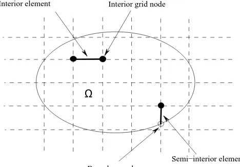
The problem domain is embedded in a Cartesian grid as shown in Figure 1. Grid points inside the problem domain are taken to be interior nodes, while boundary nodes are defined as the intersections of the grid lines and the boundaries. There are two types of elements, namely interior and semi-interior IRBFEs. An interior element is formed using two adjacent interior nodes while a semi-interior element is generated by an interior node and a boundary node.
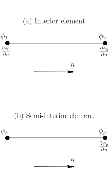
2.1. Interior elements
Consider an interior element,η ∈[η1, η2], and its two nodes are locally named as 1 and 2. Let φ(η) be a function andφ1, ∂φ1/∂η,φ2 and ∂φ2/∂η be the values ofφ and ∂φ/∂η at the two
derivative of φ(η) using two multiquadric (MQ) functions whose centres are located at η1
and η2
∂2φ ∂η2(η) =
d2φ
dη2(η) =w1
q
(η−η1)2+a21 +w2
q
(η−η2)2+a22 =w1I1(2)(η) +w2I2(2)(η), (7)
where Ii(2)(η) conveniently denotes the MQ, wi and ai are the associated weight and MQ-width at node i (i = {1,2}). We simply take ai = βh, where h is a grid size and β is a factor.
First-order derivative of φ and the function φ are approximated by integrating (7) with respect to η
∂φ ∂η(η) =
dφ
dη(η) = w1I (1)
1 (η) +w2I2(1)(η) +C1, (8) φ(η) =w1I1(0)(η) +w2I2(0)(η) +C1η+C2, (9)
where Ii(1)(η) = R Ii(2)(η)dη, Ii(0)(η) = R Ii(1)(η)dη, and C1 and C2 are the constants of
integration. By collocating (9) and (8) atη1 andη2, the relation between the physical space
and the RBF coefficient space is obtained
φ1 φ2 ∂φ1 ∂η ∂φ2 ∂η
| {z } b φ =
I1(0)(η1) I2(0)(η1) η1 1 I1(0)(η2) I2(0)(η2) η2 1 I1(1)(η1) I2(1)(η1) 1 0 I1(1)(η2) I2(1)(η2) 1 0
| {z }
I w1 w2 C1 C2
| {z } b
w
, (10)
where φbis the nodal-value vector, I the conversion matrix, and wb the coefficient vector. It is noted that not only the nodal values of φ but also of ∂φ/∂η are incorporated into the conversion system and this imposition is done in an exact manner owing to the presence of integration constants. Solving (10) yields
b
Substitution of (11) into (9), (8) and (7) leads to
φ(η) =hI1(0)(η), I2(0)(η), η,1iI−1φ,b (12) ∂φ
∂η(η) = h
I1(1)(η), I2(1)(η),1,0iI−1φ,b (13)
∂2φ ∂η2(η) =
h
I1(2)(η), I2(2)(η),0,0iI−1φ.b (14)
They can be rewritten in the form
φ(η) =ϕ1(η)φ1+ϕ2(η)φ2+ϕ3(η) ∂φ1
∂η +ϕ4(η) ∂φ2
∂η , (15)
∂φ ∂η(η) =
dϕ1(η)
dη φ1+
dϕ2(η)
dη φ2+
dϕ3(η)
dη ∂φ1
∂η +
dϕ4(η)
dη ∂φ2
∂η , (16)
∂2φ ∂η2(η) =
d2ϕ 1(η)
dη2 φ1+
d2ϕ 2(η)
dη2 φ2+
d2ϕ 3(η)
dη2 ∂φ1
∂η +
d2ϕ 4(η)
dη2 ∂φ2
∂η , (17)
where {ϕi(η)}4i=1 is the set of basis functions in the physical space. These expressions allow
one to compute the values of φ, ∂φ/∂η, and ∂2φ/∂η2 at any point η in [η
1, η2] in terms of
four nodal unknowns, i.e. the values of the field variable and its first-order derivatives at the two extremes (also grid points) of the element.
For convenience, in the case ofη ≡x, we denote
µi =
d2ϕi(x 1)
dx2 , (18)
νi =
d2ϕi(x 2)
dx2 , (19)
and in the case of η≡y,
θi =
d2ϕi(y 1)
dy2 , (20)
ϑi =
d2ϕi(y 2)
dy2 , i={1,2,3,4}. (21)
2.2. Semi-interior elements
is given at ηb. The conversion system can be formed as φb φg ∂φg ∂η =
Ib(0)(ηb) Ig(0)(ηb) ηb 1
Ib(0)(ηg) Ig(0)(ηg) ηg 1
Ib(1)(ηg) Ig(1)(ηg) 1 0
wb wg C1 C2 . (22)
(22) leads to
φ(η) =ϕ1(η)φb+ϕ2(η)φg+ϕ3(η) ∂φg
∂η , (23)
∂φ ∂η(η) =
dϕ1(η)
dη φb+
dϕ2(η)
dη φg+
dϕ3(η)
dη ∂φg
∂η , (24)
∂2φ ∂η2(η) =
d2ϕ 1(η)
dη2 φb+
d2ϕ 2(η)
dη2 φg+
d2ϕ 3(η)
dη2 ∂φg
∂η . (25)
It can be seen that the conversion matrix in (22) is under-determined and its inverse can be obtained using the SVD technique (pseudo-inversion). Owing to the facts that point collocation is used and the RBF conversion matrix is not over-determined, the boundary condition φb is imposed in an exact manner. For other types of semi-interior elements, the reader is referred to An-Vo et al. [26] for details.
3. Derivation of C2-continuous ADI method
3.1. ADI scheme for N-S equations on a Cartesian grid
Consider a grid point P and its east, west, north and south neighbouring nodes denoted as
E, W, N and S, respectively (Figure 3). Collocating (5) and (6) at P, one obtains
∂2ψ
P
∂x2 + ∂2ψ
P
∂y2 +ωP = 0, (26)
∂ωP
∂t +
∂2ω
P
∂x2 + ∂2ω
P
∂y2 =Re
We now employ the ADI (Alternating-Direction Implicit) procedure [3, 4] to relax the time derivative term in (27) in two stages. At a time instant tn, (41) and (27) become
∂2ψn P
∂x2 + ∂2ψn
P
∂y2 +ω
n−1
P = 0, (28)
ωnP−1/2−ωnP−1
∆t/2 +
∂2ωn−1/2
P
∂x2 +
∂2ωn−1
P
∂y2 =Re
∂ψn P
∂y
∂ωPn−1/2
∂x −
∂ψn P
∂x
∂ωnP−1 ∂y
!
, (29)
ωn P −ω
n−1/2
P ∆t/2 +
∂2ωn−1/2
P
∂x2 +
∂2ωn P
∂y2 =Re ∂ψn
P
∂y
∂ωPn−1/2
∂x − ∂ψn P ∂x ∂ωn P ∂y ! . (30)
It can be seen that in the first stage, i.e. (29), ∂2ωn−1/2
P /∂x2 and ∂ω n−1/2
P /∂x are treated implicitly and ∂2ωn
P/∂y2 and ∂ωPn/∂y are treated implicitly in the second stage, i.e. (30). These derivatives and the second-order derivatives of streamfunction in (28) are typically approximated by a second-order CD scheme, e.g. [5], or HOC implicit schemes, e.g. [6, 7, 12, 27]. For instance in x-direction, one has
∂ωPn−1/2
∂x =
ωEn−1/2−ωWn−1/2
2h +O(h
2), (31)
∂2ωn−1/2
P
∂x2 =
ωEn−1/2−2ωPn−1/2+ωnW−1/2
h2 +O(h
2), (32)
∂2ψn P
∂x2 = ψn
E−2ψnP +ψWn
h2 +O(h
2), (33)
or
1 6
∂ωWn−1/2
∂x +
2 3
∂ωnP−1/2
∂x +
1 6
∂ωnE−1/2
∂x =
ωEn−1/2−ωWn−1/2
2h +O(h
4), (34)
1 12
∂2ωn−1/2
W
∂x2 +
10 12
∂2ωn−1/2
P
∂x2 +
1 12
∂2ωn−1/2
E
∂x2 =
ωEn−1/2−2ωPn−1/2+ωWn−1/2
h2 +O(h
4), (35)
1 12
∂2ψn W
∂x2 +
10 12
∂2ψn P
∂x2 +
1 12
∂2ψn E
∂x2 = ψn
E −2ψPn +ψnW
h2 +O(h
4). (36)
3.2. Proposed C2-continuous IRBFE-ADI method
As in Figure 3, one can form 4 two-node IRBFEs associated with P, namely W P,P E, SP
and P N, assumed to be interior elements. To approximate ∂2ψn
P/∂x2 and ∂2ω n−1/2
P /∂x2,
∂2ψn
P/∂y2 and ∂2ωnP/∂y2 via (17), we propose to use the elements W P, SP, respectively, with abbreviations (19) and (21),
∂2ψn P
∂x2 =ν1ψ
n
W +ν2ψPn+ν3 ∂ψn
W
∂x +ν4 ∂ψn
P
∂x , (37)
∂2ωn−1/2
P
∂x2 =ν1ω
n−1/2
W +ν2ωPn−1/2+ν3
∂ωnW−1/2
∂x +ν4
∂ωPn−1/2
∂x , (38)
∂2ψn P
∂y2 =ϑ1ψ
n
S+ϑ2ψPn+ϑ3 ∂ψn
S
∂y +ϑ4 ∂ψn
P
∂y , (39)
∂2ωn P
∂y2 =ϑ1ω
n
S+ϑ2ωPn+ϑ3 ∂ωn
S
∂y +ϑ4 ∂ωn
P
∂y . (40)
It will be shown later thatC2-continuous conditions are imposed atP in bothx- andy-grid
lines. As a result, instead of using element W P to give approximations of ∂2ψn
P/∂x2 and
∂2ωn−1/2
P /∂x2, we are able to use element P E as a replacement. Similarly, element P N can replaceSP to give approximations for∂2ψn
P/∂y2 and∂2ωnP/∂y2. These possibilities will give the same results. Substituting (37) and (39) into (28), (38) into (29), and (40) into (30), we have
ν1ψnW +ϑ1ψnS+ (ν2+ϑ2)ψPn +ν3 ∂ψn
W
∂x +ϑ3 ∂ψn
S
∂y +ν4 ∂ψn
P
∂x +ϑ4 ∂ψn
P
∂y =ω
n−1
P , (41)
ν1ωWn−1/2+ (ν2+
1 ∆t/2)ω
n−1/2
P +ν3
∂ωWn−1/2
∂x + (ν4 −Re ∂ψn
P
∂y )
∂ωPn−1/2
∂x =
ωnP−1
∆t/2 −
∂2ωn−1
P
∂y2 −Re
∂ψn P
∂x
∂ωPn−1
∂y , (42)
ϑ1ωSn+ (ϑ2+
1 ∆t/2)ω
n P +ϑ3
∂ωn S
∂y + (ϑ4+Re ∂ψn P ∂x ) ∂ωn P ∂y =
ωPn−1/2
∆t/2 −
∂2ωn−1/2
P
∂x2 +Re
∂ψn P
∂y
∂ωPn−1/2
∂x . (43)
Thus, at a nodal point P in (41) there are three unknowns, namely ψn
P, ∂ψPn/∂x and
∂ψn
P/∂y. To solve (41), two additional equations are needed and devised here by impos-ing C2-continuous conditions at P inx- and y-directions, i.e.
∂2ψn
P ∂x2 L = ∂2ψn
P ∂x2 R , (44) ∂2ψn
P ∂y2 B = ∂2ψn
P
∂y2
T
where (.)L indicates that the computation of (.) is based on the element to the left of P, i.e. element WP, and similarly subscript R,B,T denotes the right (PE), bottom (SP) and top (PN) elements. The left of equations (44) and (45) are replaced by (37) and (39) and the right by similar expressions obtained via (17), noting (18) and (20) respectively, yielding
ν1ψWn +ν2ψPn +ν3 ∂ψn
W
∂x +ν4 ∂ψn
P
∂x =µ1ψ
n
P +µ2ψEn +µ3 ∂ψn
P
∂x +µ4 ∂ψn
E
∂x , (46)
ϑ1ψSn+ϑ2ψPn +ϑ3 ∂ψn
S
∂y +ϑ4 ∂ψn
P
∂y =θ1ψ
n
P +θ2ψnN +θ3 ∂ψn
P
∂y +θ4 ∂ψn
N
∂y . (47)
At the nodal pointP and for the vorticity field, in the first relaxation stage in thex-direction, there are two unknowns in (42), namely ωPn−1/2 and ∂ωPn−1/2/∂x and in the second stage of relaxation in the y-direction, two unknowns in (43), namely ωn
P and∂ωPn/∂y. To solve (42), one additional equation is needed and also devised by imposing C2-continuity condition at P inx-direction, i.e.
∂2ωPn−1/2 ∂x2
!
L = ∂
2ωn−1/2
P
∂x2
!
R
. (48)
The left of equation (48) is replaced by (38) and the right by a similar expression obtained via (17), noting (18), yielding
ν1ωWn−1/2+ν2ωPn−1/2+ν3
∂ωWn−1/2 ∂x +ν4
∂ωPn−1/2
∂x =µ1ω
n−1/2
P +µ2ωEn−1/2+µ3
∂ωPn−1/2 ∂x +µ4
∂ωEn−1/2
∂x .
(49) In a similar manner, to solve (43), one additional equation is created by imposing C2
-continuity condition atP in y-direction, i.e.
∂2ωn
P ∂y2 B = ∂2ωn
P
∂y2
T
, (50)
The left of equation (50) is replaced by (40) and the right by a similar expression obtained via (17), noting (20), yielding
ϑ1ωnS+ϑ2ωPn +ϑ3 ∂ωn
S
∂y +ϑ4 ∂ωn
P
∂y =θ1ω
n
P +θ2ωNn +θ3 ∂ωn
P
∂y +θ4 ∂ωn
N
∂y . (51)
For the vorticity field, it can be seen from (42), (43), (49) and (51) that there are 4 nonzero entries for the governing equations, i.e. (42) and (43), and 6 nonzero entries for the C2
-continuity conditions at the grid point P, i.e. (49) and (51). At the first relaxation stage, collection of equations (42) and (49) at nodal points on each and every x-grid line leads to Ny independent sets of equations. Each set contains 2Nx equations for 2Nx unknowns associated with an x-grid line with Nx nodes. At the second stage, collection of equations (43) and (51) at nodal points on each and every y-grid line leads to Nx independent sets of equations. Each set contains 2Ny equations for 2Ny unknowns associated with a y-grid line with Ny nodes. In contrast to the direct solution approaches in [26, 29] where a system of 3N equations for 3N unknowns are required, the current approach results in considerable savings in terms of both storage and computational time. The latter is significantly reduced further when parallelisation is implemented to independently solve these relatively small sets of 2Nη equations.
At high values of theRe, the fourth terms on the LHS of (42) and (43) are dominant, which guarantees diagonally dominant system matrices. Owing to the fact that two-node IRBFEs are used, the proposed method also leads to very sparse systems and its solution is a C2
function across IRBFEs.
4. Numerical examples
The performance of the proposedC2-continuous IRBFE-ADI method is studied through the
simulation of flows in square and triangular cavities. For all numerical examples presented in this study, the MQ shape parameter ais simply chosen proportionally to the element length
h by a factorβ. β = 1 is used throughout the computations. In the case of non-rectangular domains, there may be some nodes that are too close to the boundary. If an interior node falls within a distance of h/4 to the boundary, such a node is removed from the set of nodal points. A steady solution is obtained with a time marching approach starting from a computed solution at a lower Reynolds number. For the special case of Stokes equation, the starting condition is the rest state.
The solution procedure involves the following steps
flow. Otherwise, take the solution of a lower Reynolds number as an initial guess.
(2) Discretise the streamfunction equation at a time instanttn(28) by means ofC2-continuous
IRBFEs, i.e. (41), (46) and (47), and then apply the LU technique to factorise the system matrix into two triangular matrices. It is noted that the factorisation needs to be done only once.
(3) Solve (28) subjects to boundary conditions for the new streamfunction field.
(3) Derive a computational boundary condition for the vorticity from the updated stream-function field.
(4) Solve for the new vorticity field in two stages by using (42) and (49), (43) and (51) in x -and y-directions respectively.
(5) Check to see whether the solution has reached a steady state through a condition on convergence measure
CM(ψ) =
s
N
P
i=1
(ψi−ψ0i)2
s
N
P
i=1 ψ2
i
<10−9, (52)
where N is the total number of grid nodes.
(6) IfCM is not satisfactorily small, advance pseudo-time and repeat from step (3). Other-wise, stop the computation and output the results.
4.1. Square cavity
Square cavity flow is the most studied case in the literature of internal flows. This type of flow is important firstly in its own right as a basic physical model. Then, owing to its simple geometry and rich flow physics at different Reynolds numbers, the problem also serves as a useful test for numerical algorithms in CFD. The cavity is taken to be a unit square, with the lid sliding from left to right at a unit velocity. The boundary conditions can be specified as
ψ = 0, ∂ψ/∂x= 0 on x= 0, x= 1,
ψ = 0, ∂ψ/∂y = 0 on y= 0,
ψ = 0, ∂ψ/∂y = 1 on y= 1.
normal to the boundary), are used to derive computational boundary conditions for ω in solving (6). Making use of (5), the values of ω on the boundaries are computed by
ωb =−
∂2ψ
b
∂x2 on x= 0, x= 1, (53)
ωb =−
∂2ψ
b
∂y2 on y= 0, y = 1. (54)
In computing (53) and (54), one needs to incorporate∂ψb/∂xinto∂2ψb/∂x2, and∂ψb/∂y into
∂2ψ
b/∂y2, respectively. A simple technique to derive ωbin the context of 2-node IRBFEs can be found in [29]. It will be briefly reproduced here for the sake of completeness. Assuming that node 1 and 2 of an IRBFE are a boundary node and an interior grid node respectively (i.e. 1≡b and 2≡g). Boundary values of the vorticity are obtained by applying (17) as
ωb =−
∂2ψ
b
∂η2 =−
d2ϕ 1(ηb)
dη2 ψb +
d2ϕ 2(ηb)
dη2 ψg+
d2ϕ 3(ηb)
dη2 ∂ψb
∂η +
d2ϕ 4(ηb) dη2
∂ψg
∂η
, (55)
where η represents x and y; ψb and ∂ψb/∂η are the Dirichlet and Neumann boundary con-ditions for ψ, and ψg and ∂ψg/∂η are known values taken from the solution of the stream-function equation (5). It is noted that (i) all given boundary conditions are imposed in an exact manner; and (ii) this technique only requires the local values of ψ and ∂ψ/∂η at the boundary node and its adjacent grid node to estimate the Dirichlet boundary conditions for the vorticity equation (6).
It can be seen that there are two values of u at each top corner of the cavity making the solution singular. In the well-known paper by Ghia et al. [30], the flow was simulated by the finite-difference scheme and a multigrid method using very fine grids (i.e. 129×129 and 257×257). The obtained results are very accurate and they have been considered as a benchmark of finite-difference methods. In the later work by Botella and Peyret [31], the regular and singular parts of the solution are handled by a Chebyshev collocation and an analytic method respectively. Benchmark spectral results for the flow at Re = 100 and
Re= 1000 were reported. In the present study, the set of 2-node IRBFEs is generated from grid lines that pass through interior grid nodes. As a result, the set of interpolation points does not include the top corners of the cavity and hence corner singularities do not explicitly enter the discrete system.
so-lutions, i.e. Ghia et al. [30] and Botella and Peyret [31], and with the global 1D-IRBF collocation (1D-IRBF-C) results recently given in Mai-Duy and Tran-Cong [32]. These com-parisons aim to assess the accuracy of the present method. To assess the efficiency and stability, an ADI method where streamfunction and vorticity are discretised by a three-node CD is also implemented. We denote this method as CD-ADI. It is noted that the same method of deriving computational vorticity boundary conditions is used in both IRBFE-ADI and CD-ADI methods.
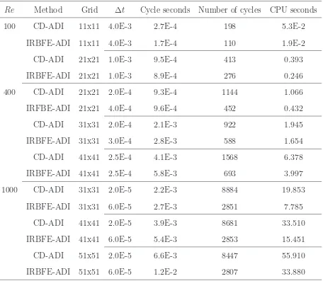
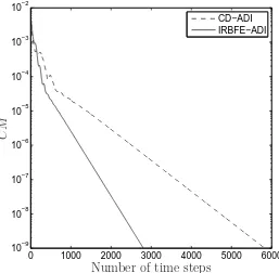
Time-stepping convergence: The convergence behaviours of IRBFE-ADI and CD-ADI with respect to time are shown in Figures 4-6 and Table 1. It can be seen that solutions converge faster and larger time steps can be used for the present IRBFE-ADI method. The numbers of iterations are about 2.8×10³ and 5.8×10³ to reachCM <10−9 for IRBFE-ADI
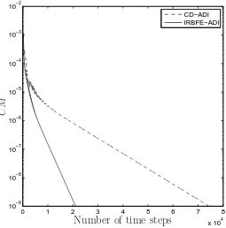
and CD-ADI respectively in the case of Re = 1000 and a grid of 51×51 (Figure 4). In the case of Re= 3200 and a grid of 91×91 (Figure 5), IRBFE-ADI takes about 2.1×10⁴
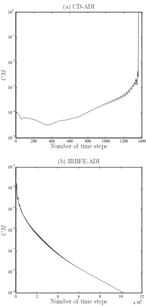
to have CM < 10−9 while CD-ADI requires about 7.4×10⁴ to have the same CM. At Re = 7500, in contrast to the IRBFE-ADI method (∆t = 1×10⁻⁶), the CD-ADI method
diverges even with a smaller time step of 5× 10⁻⁷ as shown in Figure 6. The numbers
of iterations in IRBFE-ADI method are generally lower than in CD-ADI method, yielding shorter computational time (Table 1). It is noted that the Thomas algorithm is used to solve tridiagonal systems in CD-ADI method and CPU seconds are associated with a computer which has 3.25 GB of RAM and one Intel(R) Core(TM)2 Duo CPU of 3.0 GHz. All codes are written in MATLABr language.
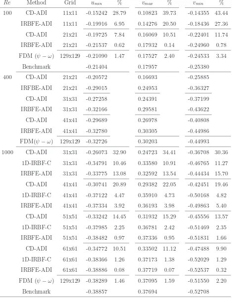
Grid-size convergence: The convergence of extrema of the vertical and horizontal velocity profiles along the centrelines of the cavity with respect to grid refinement is presented in Table 2. Benchmark results by Ghia et al. [30] and Botella and Peyret [31] are also included for comparison purposes. It can be seen that errors relative to the benchmark results are consistency reduced as the grid is refined (Re = 100,1000); and (ii) extrema values very close to the benchmark values are obtained with relatively coarse grids (e.g. 21× 21 for
Re= 100, 41×41 for Re= 400 and 61×61 for Re= 1000).
1D-IRBF-C results. Errors relative to the benchmark spectral results are less than 1% for
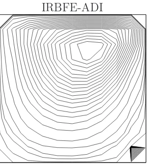
Re = 100 using a grid of 21×21 and for Re = 1000 using a grid of 61× 61. It can be seen from Figs 7-11 that smooth contours are obtained in the present IRBFE-ADI method for both the streamfunction and vorticity fields at relatively coarse grids. In Figure 7, the IRBFE-ADI method captures the primary vortex and the bottom-right corner eddy better than the CD-ADI method at Re = 100 and a grid of 11×11. With the same grids, CD-ADI method yields oscillatory contours especially for the vorticity field as shown in Figures 8-10. Converged velocity profiles at Re= 1000 and Re= 3200 are obtained by IRBFE-ADI method with grids of 51×51 and 91×91, respectively, as shown in Figure 12.
4.2. Triangular cavity
The proposed method is further verified through the simulation of steady recirculating flow in an equilateral triangle cavity. This is an example that presents a severe test for structured grid-based numerical methods [33, 34]. Figure 13 shows the geometry of the triangular cav-ity with the boundary conditions and the coordinate system. As in the square cavcav-ity flow problem, no-slip boundary condition is imposed on the left and right boundaries, while a unit horizontal velocity is prescribed on the top boundary. Numerical studies of this problem can be categorised into structured and unstructured grid/mesh-based methods. The former includes e.g. [33, 35, 36] where a finite difference method (FDM) was employed and the equilateral triangle had to be transformed to a computational domain on an isosceles right triangle. In the latter, Jyotsna and Vanka [34] used a multigrid procedure and a control volume formulation on triangular grids. They numerically verified interesting features of the flow in the Stokes regime. Kohno and Bathe [37] presented a flow-condition-based inter-polation finite element scheme on triangular meshes to achieve solutions for high Reynolds numbers.
The imposition of boundary conditions forω on the top is similar to that used in the square cavity flow, i.e. (55). On the left and right sides, analytic formulae for computing the vorticity boundary condition on a non-rectangular boundary [38] are utilised here
ωb =−
"
1 +
tx
ty
2# ∂2ψ
b
for ax-grid line, and
ωb =−
"
1 +
ty
tx
2# ∂2ψ
b
∂y2 , (57)
for ay-grid line. In (56) and (57),tx and ty are thex- and y-components of the unit vector tangential to the boundary. The approximations in (56) and (57) require information about
ψ in one direction only and they are constructed here by means of 2-node IRBFEs, i.e. (17). No exterior/fictitious points as in [33] are involved here.
Four Cartesian grids, namely Grid 1 (1952 interior points), Grid 2 (2680 points), Grid 3 (3526 points) and Grid 4 (4486 points) as shown in Figure 14, are employed to study the convergence of the solution. Unlike FDMs [33, 35, 36], the present method does not require any coordinate transformation, making modelling simple. The flow is simulated at
Re = (0,100,200,500) where Re = U(H/3)/ν, U the lid velocity and H the cavity height (i.e. length AD in Figure 13). An alternative definition of Reynolds number wasRes =US/ν where S is the cavity side length. We have Res = 2
√
3Re. For example, Re = 500 here is equivalent to Res= 1732.
Figures 15 and 16 present contour plots of the streamfunction and vorticity fields, the stream and iso-vorticity lines look comparable to those available in the literature (e.g. [33, 37]).
Figure 17 shows the profiles ofualong the vertical centrelinex= 0 andv along the horizontal line y = 2. Results obtained in [37] are also included for comparison purposes. It can be seen that the velocity profiles obtained by Grid 1 and Grid 2 at Re = 100, and by Grid 2 and Grid 3 atRe= 200 are almost identical. The present results are in good agreement with those by the flow-conditioned-based interpolation FEM for all values of Re. The profiles of
v near the the stagnant corner at different Reynolds numbers also confirm the Stokes flow assumption of the flow field in this region (i.e. [39]).
4.3. Discussion
4.3.1. Comparison with other RBF techniques
-continuous solutions rather than the usual C0-continuous solutions. C2-continuous
stream-function field leads to smooth and highly accurate velocity field.
Unlike other conventional RBF techniques, the present technique considers both the field variables and their partial derivatives in Cartesian directions in the formulation. As a re-sult, the convection terms are naturally incorporated into the system matrices as unknowns and diagonally dominant systems are always guaranteed. Numerical results show that the present technique is very stable for high Reflows without recourse to up-winding schemes. Although the present system matrices are much larger, bigger time steps can be used and hence a smaller number of iterations are required to obtain a steady state solution. The com-putational time hence becomes competitive to those required by the conventional techniques as shown in Table 1.
4.3.2. Comparison with other conventional discretisation techniques
In terms of geometric modelling, unlike pseudo-spectral and finite-difference methods, the present Cartesian-grid technique can handle irregular domains well. In contrast to finite element and finite volumes, the pre-processing here is much more economical. Non-boundary grid points are trivially generated and the intersections between grid lines and the domain boundary can be determined as in a typical FE mesh generation [40]. For example, the intersections of anx-grid line with the boundary can be found as follows. Either an xy-plane or anxz-plane passing through thex-grid line is used and the intersection between this plane and the boundary (a curve or curves) is determined by analytic geometric methods. The intersection between the grid line and the curve(s) can then be easily determined.
the proposed ADI method are under investigation. It is pointed out that we can approach tridiagonal system matrices with the same size as those in PR-ADI for diffusion-convection type equations.
5. Concluding remarks
We propose a C2-continuous alternating direction implicit solution method for solving the
streamfunction-vorticity formulation governing fluid flows. Numerical experiments are con-ducted with problems on rectangular and non-rectangular domains. The method successfully simulates the fluid flows considered in a wide range of Reynolds numbers. Attractive fea-tures of the proposed methods include (i) simple preprocessing (Cartesian grids); (ii) a sparse system matrix (2-node approximations); and a higher order of continuity across grid nodes (C2-continuous elements). Numerical results show that (i) larger time steps can be used and
smaller numbers of iterations are required in comparison with the classical CD-ADI method; and (ii) smooth solutions and high levels of accuracy are achieved using relatively coarse grids.
Acknowledgement: D.-A. An-Vo would like to thank USQ, FoES and CESRC for a PhD scholarship. This work was supported by the Australian Research Council.
References
[1] G. D. Mallinson, G. D. V. Davis, The method of the false transient for the solution of coupled elliptic equations, Journal of Computational Physics 12 (1973) 435–461.
[2] C. Pozrikidis, Introduction to theoretical and computational fluid dynamics, Oxford University Press, 1997.
[3] D. W. Peaceman, J. H. H. Rachford, The numerical solution of parabolic and elliptic differential equations, Journal of the Society for Industrial and Applied Mathematics 3(1) (1955) 28–41.
[5] A. S. Benjamin, V. E. Denny, On the convergence of numerical solutions for 2-D flows in a cavity at large Re, Journal of Computational Physics 33 (1979) 340–358.
[6] L. Collatz, The numerical treatment of differential equations, Springer-Verlag, Berlin, 1960.
[7] R. S. Hirsh, Higher order accurate difference solution of fluid mechanics problems by a compact differencing technique, Journal of Computational Physics 19 (1975) 90–109.
[8] S. K. Lele, Compact finite difference schemes with spectral-like resolution, Journal of Computational Physics 103 (1992) 16–42.
[9] S. Karaa, J. Zhang, High order ADI method for solving unsteady convection-diffusion problems, Journal of Computational Physics 198 (2004) 1–9.
[10] S. Karaa, High-order ADI method for stream-function vorticity equations, PMMA: Proceedings in Applied Mathematics and Mechanics 7 (2007) 1025601–1025602.
[11] Y. Ma, C.-P. Sun, D. A. Haake, B. M. Churchill, C.-M. Ho, A high-order alternating direction implicit method for the unsteady convection-dominated diffusion problem, Internatioanl Journal for Numerical Methods in Fluids Early View (2011).
[12] Y. Adam, Highly accurate compact implicit methods and boundary conditions, Journal of Computational Physics 24 (1976) 10–22.
[13] D. A. You, A high order Pade ADI method for unsteady convection-diffusion equations, Journal of Computational Physics 214 (2006) 1–11.
[14] G. E. Fasshauer, Meshfree approximation methods with Matlab, Interdisciplinary math-ematical sciences, vol. 6. Singapore: World Scientific Publishers, 2007.
[15] S. N. Atluri, S. Shen, The meshless local Petrov-Galerkin (MLPG) method, Tech Science Press, 2002.
[16] C. S. Chen, A. Karageorghis, Y. S. Smyrlis, The method of fundamental solutions - A meshless method, Dynamic Publishers, 2008.
[18] N. Mai-Duy, T. Tran-Cong, Numerical solution of differential euqations using multi-quadric radial basis function networks, Neural Networks 14 (2001) 185–199.
[19] N. Mai-Duy, R. Tanner, Solving high order partial differential equations with indirect radial basis function networks, International Journal for Numerical Method in Engi-neering 63 (2005) 1636–1654.
[20] N. Mai-Duy, T. Tran-Cong, An effective indirect RBFN-based method for numerical solution of PDEs, Numerical Methods for Partial Differential Equations 21 (2005) 770– 790.
[21] A. H. D. Cheng, M. A. Golberg, E. J. Kansa, G. Zammito, Exponential convergence and h-c multiquadric collocation method for partial differential equations, Numerical Methods for Partial Differential Equations 19 (2003) 571–594.
[22] C.-S. Huang, C.-F. Lee, A.-D. Cheng, Error estimate, optimal shape factor, and high precision computation of multiquadric collocation method, Engineering Analysis with Boundary Elements 31 (2007) 614–623.
[23] C. Shu, H. Ding, K. Yeo, Local radial basis function-based differential quadrature method and its application to solve two-dimensional incompressible Navier-Stokes equa-tions, Computer Methods in Applied Mechanics & Engineering 192 (2003) 941–954.
[24] B. ˇSarler, R. Vertnik, Meshfree explicit local radial basis function collocation method for diffusion problems, Computer & Mathematics with Applications 51 (2006) 1269–1282.
[25] E. Divo, A. Kassab, An efficient localized radial basis function meshless method for fluid flow and conjugate heat transfer, Journal of Heat Transfer 129 (2007) 124–136.
[26] D.-A. An-Vo, N. Mai-Duy, T. Tran-Cong, A C2-continuous control-volume technique
based on Cartesian grids and two-node integrated-RBF elements for second-order elliptic problems, CMES: Computer Modeling in Engineering and Sciences 72 (4) (2011) 299– 334.
[28] P. K. Khosla, S. G. Rubin, A diagonally dominant second-order accurate implicit scheme, Computers and Fluids 2 (2) (1974) 207–209.
[29] D.-A. An-Vo, N. Mai-Duy, T. Tran-Cong, High-order upwind methods based on C2
-continuous two-node integrated elements for viscous flows, CMES: Computer Modeling in Engineering and Sciences 80 (2) (2011) 141–177.
[30] U. Ghia, K. N. Ghia, C. Shin, High-Re Solutions for Incompressible Flow Using the Navier-Stokes equations and a Multigrid method, Journal of Computational Physics 48 (1982) 387–411.
[31] O. Botella, R. Peyret, Benchmark spectral results on the lid-driven cavity flow, Com-puters & Fluids 27 (1998) 421–433.
[32] N. Mai-Duy, T. Tran-Cong, A high-order upwind control-volume method based on integrated RBFs for fluid-flow problems, International Journal for Numerical Methods in Fluids 67 (2011) 1973–1992.
[33] C. J. Ribbens, L. T. Watson, C.-Y. Wang, Steady viscous flow in a triangular cavity, Journal of Computational Physics 112(1) (1994) 173–181.
[34] R. Jyotsna, S. P. Vanka, Multigrid calculation of steady, viscous flow in a triangular cavity, Journal of Computational Physics 122 (1995) 107–117.
[35] M. Li, T. Tang, Steady viscous flow in a triangular cavity by efficient numerical tech-niques, Computers and Mathematics with Applications 31(10) (1996) 55–65.
[36] E. Erturk, O. Gokcol, Fine grid numerical solutions of triangular cavity flow, The European Physical Journal - Applied Physics 38 (2007) 97–105.
[37] H. Kohno, K. Bathe, A flow-condition-based interpolation finite element procedure for triangular grids, International Journal for Numerical Method in Fluids 51 (2006) 673–699.
[39] H. K. Moffat, Viscous and resistive eddies near a sharp corner, Journal of Fluid Mechanics 18 (1963) 1–18.
[40] J. F. Thompson, B. K. Soni, N. P. Weatherill, Handbook of grid generation, CRC Press, 1999.
[41] N. Mai-Duy, T. Tran-Cong, Integrated radial-basis-function networks for computing Newtonian and non-Newtonian fluid flows, Computers & Structures 87 (2009) 642–650.
Table 1: Lid-driven cavity flow: computational times.
Re Method Grid ∆t Cycle seconds Number of cycles CPU seconds
100 CD-ADI 11x11 4.0E-3 2.7E-4 198 5.3E-2
IRBFE-ADI 11x11 4.0E-3 1.7E-4 110 1.9E-2
CD-ADI 21x21 1.0E-3 9.5E-4 413 0.393
IRBFE-ADI 21x21 1.0E-3 8.9E-4 276 0.246
400 CD-ADI 21x21 2.0E-4 9.3E-4 1144 1.066
IRFBE-ADI 21x21 4.0E-4 9.6E-4 452 0.432
CD-ADI 31x31 2.0E-4 2.1E-3 922 1.945
IRBFE-ADI 31x31 3.0E-4 2.8E-3 588 1.654
CD-ADI 41x41 2.5E-4 4.1E-3 1568 6.378
IRBFE-ADI 41x41 2.5E-4 5.8E-3 693 3.997 1000 CD-ADI 31x31 2.0E-5 2.2E-3 8884 19.853
Table 2: Lid-driven cavity flow: extrema of the vertical and horizontal velocity profiles along the centrelines of the cavity. % denotes percentage errors relative to the benchmark spectral results [31]. Results of the global 1D-IRBF-C, FDM and Benchmark are taken from [41], [30] and [31] respectively.
Re Method Grid umin % vmax % vmin %
100 CD-ADI 11x11 -0.15242 28.79 0.10823 39.73 -0.14355 43.44 IRBFE-ADI 11x11 -0.19916 6.95 0.14276 20.50 -0.18436 27.36 CD-ADI 21x21 -0.19725 7.84 0.16069 10.51 -0.22401 11.74 IRBFE-ADI 21x21 -0.21537 0.62 0.17932 0.14 -0.24960 0.78 FDM (ψ−ω) 129x129 -0.21090 1.47 0.17527 2.40 -0.24533 3.34
Benchmark -0.21404 0.17957 -0.25380
400 CD-ADI 21x21 -0.20572 0.16693 -0.25885 IRFBE-ADI 21x21 -0.29015 0.24953 -0.36327 CD-ADI 31x31 -0.27258 0.24391 -0.37199 IRBFE-ADI 31x31 -0.32166 0.29581 -0.43622 CD-ADI 41x41 -0.29689 0.26978 -0.40808 IRBFE-ADI 41x41 -0.32780 0.30305 -0.44986 FDM(ψ−ω) 129x129 -0.32726 0.30203 -0.44993
1000 CD-ADI 31x31 -0.26073 32.90 0.24723 34.41 -0.36708 30.36 1D-IRBF-C 31x31 -0.34791 10.46 0.33580 10.91 -0.46765 11.27 IRBFE-ADI 31x31 -0.33775 13.08 0.32592 13.54 -0.44434 15.70 CD-ADI 41x41 -0.30741 20.89 0.29382 22.05 -0.42451 19.46 1D-IRBF-C 41x41 -0.37122 4.47 0.35910 4.73 -0.50168 4.82 IRBFE-ADI 41x41 -0.37334 3.92 0.36193 3.98 -0.49863 5.40 CD-ADI 51x51 -0.33242 14.45 0.31932 15.29 -0.45556 13.57 1D-IRBF-C 51x51 -0.37985 2.25 0.36781 2.42 -0.51469 2.35 IRBFE-ADI 51x51 -0.38482 0.97 0.37336 0.95 -0.51831 1.66 CD-ADI 61x61 -0.34772 10.51 0.33502 11.12 -0.47488 9.90 1D-IRBF-C 61x61 -0.38366 1.26 0.37173 1.38 -0.52029 1.29 IRBFE-ADI 61x61 -0.38886 0.08 0.37719 0.07 -0.52537 0.32 FDM (ψ−ω) 129x129 -0.38289 1.46 0.37095 1.59 -0.51550 2.20
Ω
Semi−interior element Interior grid node
Interior element
[image:26.595.219.453.314.477.2]Boundary node
(a) Interior element
η
φ1 φ2
∂φ1
∂η
∂φ2
∂η
(b) Semi-interior element
η
φb φg
∂φg
[image:27.595.219.396.225.513.2]∂η
P
W E
S N
[image:28.595.212.418.304.490.2]x y
0 1000 2000 3000 4000 5000 6000 10−9
10−8 10−7 10−6 10−5 10−4 10−3 10−2
CD−ADI IRBFE−ADI
C
M
[image:29.595.172.429.262.514.2]Number of time steps
Figure 4: Lid-driven cavity flow, Re= 1000, 51×51: convergence behaviour. IRBFE-ADI method using a
time step of 6×10⁻⁵converges faster than the CD-ADI method using a time step of 3×10⁻⁵. It is noted that the latter diverges for time steps greater than 3×10⁻⁵. CM denotes the relative norm of the difference
0 1 2 3 4 5 6 7 8
x 104 10−9
10−8 10−7 10−6 10−5 10−4 10−3 10−2
CD−ADI IRBFE−ADI
Number of time steps
C
[image:30.595.172.427.260.518.2]M
Figure 5: Lid-driven cavity flow,Re= 3200, 91×91, solution atRe= 1000 used as initial guess: convergence
behaviour. IRBFE-ADI method using a time step of 7×10⁻⁶
converges faster than the CD-ADI method using a time step of 2×10⁻⁶
. It is noted that the latter diverges for time steps greater than 2×10⁻⁶
. CM
0 200 400 600 800 1000 1200 1400 10−5
10−4 10−3 10−2 10−1 100
Number of time steps
C
M
(a) CD-ADI
0 2 4 6 8 10 12
x 104 10−9
10−8 10−7 10−6 10−5 10−4 10−3
Number of time steps
C
M
[image:31.595.158.444.80.681.2](b) IRBFE-ADI
Figure 6: Lid-driven cavity flow, Re = 7500, 131×131, solution at Re = 5000 used as initial guess:
convergence behaviour. CD-ADI method uses a time step of 5×10⁻⁷
and IRBFE-ADI method uses a time step of 1×10⁻⁶
. CM denotes the relative norm of the difference of the streamfunction fields between two
CD-ADI IRBFE-ADI
Figure 7: Lid-driven cavity flow, Re = 100, grid = 11×11: streamlines. The contour values for CD-ADI
(a) CD-ADI
ψ ω
(b) IRBFE-ADI
[image:33.595.140.535.126.619.2]ψ ω
Figure 8: Lid-driven cavity flow, Re = 1000, grid = 51×51: stream and iso-vorticity lines. The contour
(a) CD-ADI
ψ ω
(b) IRBFE-ADI
[image:34.595.95.531.137.613.2]ψ ω
Figure 9: Lid-driven cavity flow, Re = 3200, grid = 91×91: stream and iso-vorticity lines. The contour
(a) CD-ADI
ψ ω
(b) IRBFE-ADI
[image:35.595.138.534.142.610.2]ψ ω
Figure 10: Lid-driven cavity flow,Re= 5000, grid = 111×111: stream and iso-vorticity lines. The contour
ψ ω
Figure 11: Lid-driven cavity flow, IRBFE-ADI,Re= 7500, grid = 131×131: stream and iso-vorticity lines.
(a) Re= 1000, grid= 51×51
−0.50 0 0.5 1
0.1 0.2 0.3 0.4 0.5 0.6 0.7 0.8 0.9 1
0 0.2 0.4 0.6 0.8 1
−0.6 −0.5 −0.4 −0.3 −0.2 −0.1 0 0.1 0.2 0.3 0.4 Benchmark [31] IRBFE−ADI CD−ADI Benchmark [31] IRBFE−ADI CD−ADI u y x v
(b) Re= 3200, grid= 91×91
−0.50 0 0.5 1
0.1 0.2 0.3 0.4 0.5 0.6 0.7 0.8 0.9 1
0 0.2 0.4 0.6 0.8 1
−0.8 −0.6 −0.4 −0.2 0 0.2 0.4 0.6
Ghia et al.[30] IRBFE−ADI CD−ADI
[image:37.595.110.533.184.663.2]Ghia et al.[30] IRBFE−ADI CD−ADI u y x v
−20 −1.5 −1 −0.5 0 0.5 1 1.5 2 0.5
1 1.5 2 2.5 3 3.5 4
x
y
A
B D C
(ψ = 0, ∂ψ/∂n= 0) (ψ = 0, ∂ψ/∂n = 0)
[image:38.595.160.442.248.535.2](ψ = 0, ∂ψ/∂n= 1)
Grid 1 Grid 2
[image:39.595.108.536.204.609.2]Grid 3 Grid 4
Re= 0, Grid 1 Re= 100, Grid 2
[image:40.595.109.547.199.611.2]Re= 200, Grid 3 Re= 500, Grid 4
Re= 0, Grid 1 Re= 100, Grid 2
[image:41.595.110.544.194.611.2]Re= 200, Grid 3 Re= 500, Grid 4
Figure 16: Triangular cavity flow: iso-vorticity lines which are drawn at intervals of ∆ω= 0.5 for a range of
−1.50 −1 −0.5 0 0.5 1 1.5 0.5
1 1.5 2 2.5 3
data1 data2
Kohno and Bathe [37] Grid 1
Grid 2 data6
Re= 100
−1.50 −1 −0.5 0 0.5 1 1.5 0.5
1 1.5 2 2.5 3
data1
Kohno and Bathe [37] data3
Grid 2 Grid 3 data6
Re= 200
−1.50 −1 −0.5 0 0.5 1 1.5 0.5
1 1.5 2 2.5 3
Kohno and Bathe [37] Grid 4
data3 data4
[image:42.595.202.413.101.682.2]Re= 500
![Figure 8: Lid-driven cavity flow, Revalues are taken to be the same as those in [30] and [42] respectively](https://thumb-us.123doks.com/thumbv2/123dok_us/152580.29724/33.595.140.535.126.619/figure-lid-driven-cavity-ow-revalues-taken-respectively.webp)