Transformation of narrowband wavetrains of surface gravity waves passing over a bottom step

DOI: 10.1051/mmnp/20149505

Transformation of Narrowband Wavetrains of Surface

Gravity Waves Passing over a Bottom Step

A.R. Giniyatullin

, A.A. Kurkin

, S.V. Semin

, Y.A. Stepanyants

2 _{University of Southern Queensland, Toowoomba, Australia}

Abstract.The problem of transformation of quasimonochromatic wavetrains of surface gravity waves with narrow spatial-temporal spectra on the bottom shelf is considered in the linear approximation. By means of numerical modeling, the transmission and reflection coefficients are determined as functions of the depth ratio and wave number (frequency) of an incident wave. The approximation formulae are proposed for the coefficients of wave transformation. The characteristic features of these formulae are analyzed. It is shown that the numerical results agree quite satisfactorily with the proposed approximation formulae.

Keywords and phrases: wavetrain, wave transformation, numerical modeling, quasi-monochromatic wave, reflected and transmitted waves, bottom step

Mathematics Subject Classification: 35Q35, 65Y20, 74J05, 74J15, 76B15, 86-08

1. Introduction

The problem of surface wave transformation on the bottom shelf has an old history and is related to many practical problems. One of such problems is the calculation of the parameters of transmitted waves generated by an incident wave propagating from the open ocean towards a shore and passing over a shelf zone with the sharp bottom rise. It is well-known that in such case a significant concentration of wave energy can happen due to the wave arriving in the relatively shoal zone. In order to estimate the wave impact on the beaches, harbors, marine engineering constructions, and ships in the shelf zone it is necessary to calculate accurately the amplitude and wavelength of a transmitted wave passing over the abrupt bottom raising which may be approximated by a step. The aforementioned problem has also an academic interest, therefore many theoretical, experimental and numerical works were undertaken in attempt to find the transformation coefficients both in the linear and nonlinear cases.

The expressions for the transformation coefficients (the coefficients of wave transmission,T, and reflec-tion,R) for surfaceinfinitely long wavespropagating in the canal with sharp variation of a cross-section were derived for the first time by Lamb in the linear approximation [6]. Considering further an infinitely wide canal, we will focus on the transformation coefficients due to abrupt bottom raising only. In this

∗_{The authors adhere the principle of alphabetical order of the names. Corresponding author. E-mail:}

case Lamb’s formulae read:

T = 2

1 +p

h₂/h₁, R=

1−p h₂/h₁

1 +p

h₂/h₁, (1.1)

where T = At/Ai is the ratio of the transmitted and incident wave amplitudes andR =Ar/Ai as the

ratio of the reflected and the incident wave amplitudes; h₁ is the water depth before the bottom shelf, andh₂ is the water depth after the bottom shelf.

0.001 0.01 0.1 1 10 100 1000

1 0.5

0.5 1 1.5 2

h2 /h1 T, R

1

2 2'

Figure 1. _{Dependence of the transmission T (red line 1) and reflection R (blue line} 2) coefficients on the depth ratio h₂/h₁ for long gravity waves over shelf. Line 2′ _is

the mirror reflection of the negative branch 2 regarding the horizontal axis (i.e. the dependence of|R|onh2/h1).

The transformation coefficients depend on the water depths ratio only; their graphics are depicted in Fig. 1 in the semi-logarithmic scale. As it might be expected, when the depthsh₁andh₂ are equal, then there is no reflected wave (R= 0), and the transmission coefficient equals to one (T = 1). Ifh2/h1→0, the incident wave experiences the full reflection (R = 1), and the reflected wave has the same polarity as the incident wave. The transmission coefficient in this limiting case formally equals to two (T = 2), but in fact there is no transmitted wave; just a tight splash of zero wavelength occurs in this case at a vertical wall.

If h₂/h₁ → ∞ the full reflection of an incident wave occurs again, but in the anti-phase, so that

R → −1. In this case the amplitude of the transmitted wave asymptotically vanishes (T →0), and its wavelength grows to infinity. Hereinafter we will consider wavetrains containing many periods of the carrier wave within the envelope and will not interested in the polarity of the wavetrains. Therefore we will consider only the absolute value of the reflection coefficient.

Note that in his derivation of the transformation coefficients Lamb used simple principles of mass conservation and pressure continuity above the shelf neglecting the vertical component of fluid flow. Later Bartholomeusz [2] considered the problem rigorously for waves of arbitrary wavelength and derived an integral equation for determining the transmission coefficients. However, the equation derived was not solved in general, but was analyzed in the long-wave limit only. In this limit Lamb’s transformation coefficients directly follow from the rigorous consideration. Lamb’s formulae were re-derived also in many other papers (see, e.g., [3, 15, 20] and references therein).

limit these coefficients naturally reduce to those described by Lamb’s formulae. Note that in the nonlinear case the transformation coefficients make sense only in the vicinity of the edge of bottom step, because in the subsequent wave propagation away from the edge, both the transmitted and reflected waves undergo significant nonlinear distortions.

In the special case when the incident wave represents a soliton described by the Korteweg–de Vries (KdV) equation the problem of wave transformation on the bottom shelf can be solved completely. The local transformation on the shelf can be calculated by means of the Lamb or Mirchina & Pelinovsky formulae [6,17]. Then, if the amplitudes and characteristic widths of the transmitted and reflected waves are such that the KdV equation is still applicable to their description, then one can calculate the number and amplitudes (as well as other parameters) of secondary solitons emerging from the transmitted and reflected pulses. Such calculation was undertaken for the first time by Pelinovsky [19] (see also his monograph [20]) and then, it was reproduced by other authors (see the references in [21]). This approach is quite reasonable for waves of relatively small amplitudes, and the laboratory experiments [7, 22] have demonstrated a good agreement with the theoretical predictions in such case. For large-amplitude solitary waves the weakly nonlinear theory is inapplicable, therefore it is not surprising that the discrepancy between the experimental data and predictions of the KdV theory was observed. In particular, the wave breaking phenomenon occurred in the transmitted waves, when the amplitude of the incident wave attained the half of the water depth in the laboratory tank.

Note that the water wave propagation and transformation on the bottom shelf can be modelled by means of electro-magnetic transmission lines [4, 10]. Transmission lines can be treated as the convenient tool (a sort of the analogous computer) which allows one to study water-wave problems very easily. In particular, solitary wave transformations on the jump of line parameters have been studied theoretically and experimentally in [24]. It was also demonstrated a very good agreement between the theoretical predictions and experimental data within the range of validity of weakly nonlinear theory.

There were several attempts to obtain the transformation coefficients for linear waves of arbitrary wavelength after publication of Bartholomeusz’ work [2], see, for example, [13, 14, 16, 18, 23] (we do not consider here other works where surface wave transformation on the underwater obstacles of finite horizontal length was studied). The rigorous results were obtained by Newman for the infinite step [18] and by Massel for the finite step [14] (see also [15]). It was shown in these papers that the transformation coefficients can be obtained through the solution of an infinite set of algebraic equations for propagating and evanescent modes crowded to the step edge. In practices the infinite set of equation was truncated and reduced to the finite set of equation for the finite number of evanescent modes. The accuracy of calculations of the transformation coefficients depends on the number of modes taken into account; usually several tens of modes are quite enough for practical applications. The results obtained by this way were presented graphically in [14,15,18] and compared against a limited number of experimental data. However, any manipulation with the transformation coefficients presented graphically is very inconvenient, therefore it would be very desirable from the practical point of view to have an analytical formulae, at least approximate, which allow one to analyze the dependence of the coefficients on wavelength, frequency, depth ratio and, perhaps, other parameters.

In this paper we study the problem of surface wave transformation on the bottom step numerically for small-amplitude narrow-band wavetrains. We present the results of direct numerical simulation of gravity wave transformations as functions of the depth ratio before and after the bottom jump and wavenumber (frequency) of the incident quasi-monochromatic wave. Then we suggest relatively simple approximative formulae which interpolate numerical data with quite good accuracy.

2. Numerical modeling of surface wave transformation on a bottom shelf

Consider the quasi-monochromatic wave train of the frequencyωi and wavenumber of the incident wave

ki propagating from the depthh1 to the area with the depthh2 (see Fig. 2).

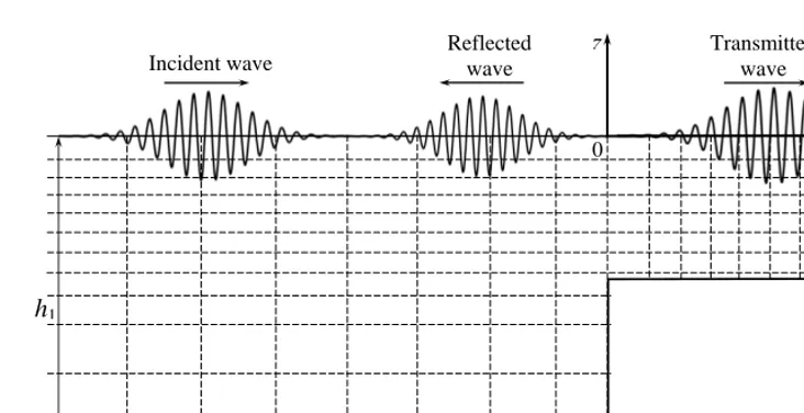
Reflected wave

Incident wave Transmitted _wave

h1

h2 z

x 0

Figure 2. _{Schematic sketch of wavetrain transformation on the bottom shelf and the} non-uniform mesh used in the numerical calculations.

denote here the derivatives onxandz, correspondingly. The basic hydrodynamic equations in the linear approximation reduce to the Laplace equation for the potential:

∆ϕ= 0, ∀t, (2.1)

and the boundary conditions are:

ϕz(t, x,−h1) = 0, at x <0; ϕz(t, x,−h2) = 0, at x >0; (2.2)

ϕx(t,0, z) = 0, at x= 0₋ and −h₁< z <−h₂; (2.3)

ηt=ϕz, and ϕt+gη= 0, at z= 0 and ∀x, (2.4)

where η(x, t) is the disturbance of the free surface, andg is the acceleration due to gravity. On the side walls of the calculation domain the “sponge boundary conditions” completely suppressing reflected waves were used.

The numerical modeling of wave transformation on the bottom shelf was undertaken with the help of MITgcm program based on the PC platform in the multi-thread mode. The program solves the Navier– Stocks equation jointly with the continuity equation for an incompressible fluid and accounts for the non-hydrostatic pressure. The detailed description of the numerical algorithm can be found in the papers [1, 11, 12].

We considered the two-dimensional model of the basin in the vertical x, z-plane with the minimum allowable number of calculation layers (just one layer) in the transverse direction to this plane. The modelled fluid (water) was assumed to be homogeneous and inviscid so that the heat and diffusion processes were absent. The length and height of the calculation domain were different in run depending on the wavelength of incident wave. The water depth h1 in the domain of incoming wave (before the bottom shelf) (see Fig. 2) was fixed and equal 50.0 m, whereas the depth after the shelf varied such that the depth ratio ranged within the interval 10−2_≤h

2/h1≤102. The horizontal size of the calculation domain was taken such that in each run the length in front of the shelf and behind it was 36 times greater than wavelength of the incident and transmitted waves, correspondingly. The absorbing boundary conditions were used on the vertical sides of the calculation domain.

the courser mesh to the finer mesh was used around the shelf position. The vertical resolution was also non-uniform with the number of grid points from 110 in the deepest domain to 30 in the shallowest domain.

The incident wavetrain was taken in the form:

η(x,0) =Aexp

−x2

D2

cosk1x; (2.5)

φ(x, z,0) =A r

2g

k₁sinh 2k₁h₁exp

−x2

D2

sink₁xcoshk₁(z+h₁). (2.6) The wave amplitudeAwas chosen to be small enough to meet the condition of the linear approximation:

A = min{h₂, h₁}/500. The incident wave wavenumber was varied, and the characteristic width of wavetrain envelope was set to be equalD= 12π/ki= 6λi.

The results of calculations are presented in Figs. 3a) and 3b) for three different wavenumbers of the incident wave: ki = 0.2, 2.0, 20.0 m−1; this corresponds to the following dimensionless wavenumbers:

κ ≡ kih₁ = 0.1, 1.0, 10.0 (we present here the results for only these three characteristic values of

κ, whereas the results were obtained for some other values of κ). In the same figures we present the graphics of transformation coefficients as per Lamb’s formulae (see red lines with the label 0). As one can see there is a big discrepancy between the Lamb formulae for infinitely long waves and numerical data for the waves of relatively small wavelength (see the data forκ= 1 and especially forκ= 10). In the meantime, whenκbecomes much less then one, Lamb’s formulae agree well with the numerical data (cf., e.g., red lines 0 and black rectangles in Figs. 3).

As has been mentioned in the Introduction, there are no analytical expressions for the transformation coefficient in the general case for arbitrary values ofκ. These coefficients can be calculated by means of the approaches described in [2,14,15], however it is impractical as it takes significant efforts and numerical calculations. Below we suggest the approximative formulae which agree with the numerical data fairly well; the formulae can be readily used for practical calculations of the transformation coefficients with relatively small errors.

3. Approximative formulae for surface waves transformation on a bottom shelf

Note first that Lamb’s formulae for the transmission and reflection coefficients can be presented in terms of wave speeds before and after the shelf:

T = 2ci

ci+ct

, |R|=|ci−ct|

ci+ct

, (3.1)

whereci=

p

gh1is the wave speed of an incident wave, andct=

p

gh2is the wave speed of a transmitted wave in the long-wave limit, kih1 ≪ 1 and kth2 ≪ 1. In this limit there is no difference between the phase and group velocities.

The relationship between the wavenumbers of transmitted and incident waves can be readily found from the condition of frequency conservation in a stationary medium. For surface gravity waves this condition reads

ω=pgktanhkh=const. (3.2)

In the long-wave approximation when Lamb’s formulae are valid we obtain from Eq. (3.2)

kt

ki

= r

h1

h₂. (3.3)

In general, the relationship between kt and ki can be found numerically from the solution of the

transcendental equation following from Eq. (3.2):

h

/h

T

0 2 3

1

a)

0.01

0.1

1

10

100

1

2

h

/h

0

1

3

2

b)

0.01

0.1

1

10

100

0.5

1

|R|

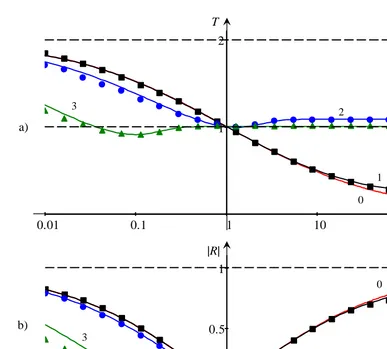
Figure 3._{The dependences of the transmission (a) and reflection (b) coefficients on the} depth ratio h₂/h₁ for surface gravity waves. Red curves 0 pertain to the shallow-water limiting case (κ→ 0) as per Lamb’s formulae (1.1). Results of numerical calculations are presented by different symbols: rectangles – κ= 0.1, dots – κ= 1 and triangles –

κ = 10. Smooth lines 1, 2 and 3 are plotted for the same values of κon the basis of approximative formulae as per Eqs. (3.6) and (3.7) (see below).

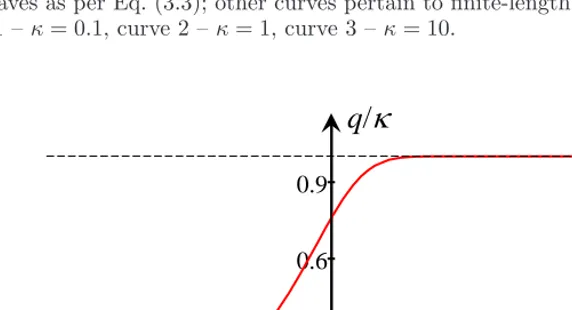
where κ = kih1 is the normalized wavenumber of the incident wave and q = kth2 is the normalized wavenumber of the transmitted wave. The dependence of the wavenumber ratio q/κon the depth ratio

h₂/h₁is shown in Fig. 4 for three values of κ= 0.1,1 and 10. Curve 1 forκ= 0.1 almost coincides with the line 0 for infinitely long waves almost everywhere; the divergence between these lines is observable only ath2/h1>100.

As it can be seen from Fig. 4, all curves asymptotically approach some constant values (q/κ)lim, when

the ratioh₂/h₁goes to infinity. The asymptotical constant values depend onκ; this is illustrated by Fig. 5. Ifκ≫1, then the hyperbolic tangents turn to unity in Eq. (3.4), and the wavenumber of the transmitted wave becomes equal to the wavenumber of the incident wave (q→κ); therefore the dependence (q/κ)lim

asymptotically approaches unity whenκ→ ∞.

The simplest way to obtain the approximative formulae for the transformation coefficients is to replace the long-wave speedsci,t in the Lamb formulae Eq. (3.1) by either group or phase velocities, which are

h

/h

q/

N

1 2 3

0

0.001

0.01

0.1

1

10

100

1000

1

2

3

4

Figure 4. _{The dependence of the dimensionless ratio of wavenumbersq/κon the depth} ratioh₂/h₁ for gravity waves in a finite depth fluid. Red curve 0 pertains to infinitely long waves as per Eq. (3.3); other curves pertain to finite-length waves as per Eq. (3.4): curve 1 –κ= 0.1, curve 2 –κ= 1, curve 3 –κ= 10.

0.01

0.1

1

10

100

0.3

0.6

0.9

1.2

N

q/

N

Figure 5. _{The dependence of (q/κ)lim onκfor surface gravity waves in the fluid of a} finite depth.

readily obtained from the dispersion relation (3.2):

Vg≡

dω dk =

ω(k) 2k

1 +khsech2kh

tanhkh

, Vp≡

ω

k =

r g

ktanhkh. (3.5)

the dimensionless variables the corresponding approximative formulae read (cf. Eqs. (1.1) and (3.1)):

T ≡ 2(Vg)i (Vg)i+ (Vg)t

= 2

1 +Q; |R| ≡

|(Vp)i−(Vp)t|

(Vp)i+ (Vp)t

=|1−κ/q|

1 +κ/q . (3.6)

where

Q=tanh (qh2/h1) + (qh2/h1)sech2(qh2/h1)

tanhκ+κsech2_κ (3.7)

Equations (3.6) and (3.7) should be considered jointly with Eq. (3.4) which binds the wavenumbers of incident and transmitted waves.

The transformation coefficients depend, in general, on the depth ratio h₂/h₁ and wavenumber of an incident wave. In the shallow-water case when bothκandqare small, Eq. (3.4) reduces toq2_/κ2_=h

1/h2 which is equivalent to Eq. (3.3) in the dimensional form. In this case the approximate formulae (3.6) and (3.7) reduce to Lamb’s formulae Eq. (1.1), and the transformation coefficients depend only on the depth ratio. Graphics of the transformation coefficients as per Eq. (3.6) are shown in Fig. 3 by smooth lines. As one can see, there is not only a qualitative agreement between the numerical data and approximative formulae, but even rather good quantitative agreement. The approximative formulae reflect well even specific features of the transformation coefficients such as the local minima in the dependenceT(h2/h1) and the limiting asymptotic values ofT andRas h₂/h₁→ ∞.

It is interesting to note that due to non-monotonic character of the dependence T(h₂/h₁), it may happen that the transmission coefficient T turns to unity not only at h₂/h₁ = 1, but also at another value ofh2/h1<1 (see, e.g., Fig. 3a) forκ= 10). At this specific value ofh2/h1the reflection coefficient is not zero, and wavelength of the transmitted wave is not equal to the wavelength of the incident wave,

q6=κ. (It is worth noting that the transformation coefficients are traditionally determined in the context of water waves on amplitudes, rather than on energies as in the quantum mechanics, thereforeT2_+R2_{6= 1} for water waves, in general.)

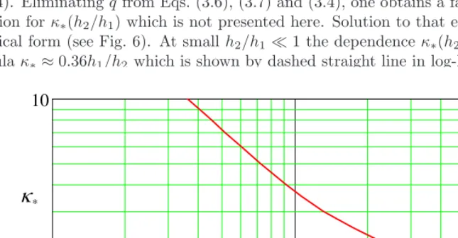
The relationship between the wavenumberκ∗of the incident wave and depth ratio when the

transmis-sion coefficient turns to unity can be found from the conditionT = 1, which should be considered jointly with Eq. (3.4). Eliminatingqfrom Eqs. (3.6), (3.7) and (3.4), one obtains a fairly complicated transcen-dental equation for κ_∗(h₂/h₁) which is not presented here. Solution to that equation is presented below in the graphical form (see Fig. 6). At smallh2/h1≪1 the dependenceκ∗(h2/h1) can be approximated by the formula κ∗≈0.36h1/h2 which is shown by dashed straight line in log-log scale in Fig. 6.

0.01

0.1

1

1

10

2 1

h h

*

N

Figure 6._{The dependence of the dimensionless wavenumberκ}

∗ of an incident wave on

4. Discussion

In spite of long history, the problem of surface waves transformation over a bottom shelf has not been completely studied thus far for waves of arbitrary wavelength in a basin of finite depth. In the long-wave approximation the analytical results were obtained only for a shallow basin [2, 3, 6, 14, 15, 17, 20] (see also [5, 8, 9, 21]).

In this paper the problem was studied numerically by means of MITgcm program [1,11,12]. The trans-formation coefficients for surface gravity waves were determined for different wavelength of an incident wave for the wide range of the depth ratios 10−2_≤h

2/h1≤102. It was discovered that the dependence of transformation coefficients on the depth ratio is non-monotonic, in general. In particular, it was shown that the amplitude of the transmitted wave may be equal to the amplitude of an incident wave not only whenh2=h1, but also at some specific ratio ofh2/h1<1; this specific ratio depends on the wavelength of the incident wave. The wavelengths of the transmitted and incident waves do not coincide in this case. The approximative formulae were proposed to interpolate the transformation coefficients and it was demonstrated that these formulae represent numerical data fairly well including specific features such as maxima and minima, as well as asymptotic values. A small discrepancy between the numerical results and approximative formulae may be caused both by the approximate character of the empirical formulae and errors of numerical calculations. We discovered, in particular, that there is better agreement between the numerical data and empirical formulae when the width of the wavetrain envelopeD increases (this can be explained by the reduction of the parasitic dispersion effect). The agreement was also improved when the numerical mesh was made finer.

Apparently, the simple exact analytical formulae for the transformation coefficients of surface gravity waves on the bottom step do not exist. In such case proposed here empirical formulae may be very useful for practical applications in physical oceanography and in other engineering sciences.

Acknowledgements. Authors are indebted to E.N. Pelinovsky for useful advices and discussions. The study was supported by the Ministry of Education and Science of Russian Federation, Project No 14.B37.21.0881.

References

[1] J. Adcroft et al. MITgcm User Manual. MIT Department of EAPS, Cambridge, MA, 2008.

[2] L.F. Bartholomeusz.The reflection of long waves at a step. Proc. Camb. Philos. Soc., 54 (1958), 106–118.

[3] G.P. Germain.Coefficients de r´eflexion et de transmission en eau peu profonde. Instytut Budownictwa Wodnego, Gdansk, Rozprawy Hydrotechniczne, Rep. no. 46, 5–13 (in French).

[4] K.A. Gorshkov, L.A. Ostrovsky, V.V. Papko, E.N. Pelinovsky.Electromodeling of finite amplitude water waves. Bull. Roy. Soc. New Zealand, 15 (1976), 123–131.

[5] R. Grimshaw, E. Pelinovsky, T. Talipova.Fission of a weakly nonlinear interfacial solitary wave at a step. Geophys. Astrophys. Fluid Dyn., 102 (2008), no. 2, 179–194.

[6] H. Lamb. Hydrodynamics. 6-th ed., Cambridge Univ. Press, Cambridge, 1932.

[7] M.A. Losada, C. Vidal, R. Medina.Experimental study of the evolution of a solitary wave at the abrupt junction.

J. Geophys. Res., 94 (1989), no. C10, 14, 557–14, 566.

[8] V.Maderich, T. Talipova, R. Grimshaw, E. Pelinovsky, B. H. Choi, I. Brovchenko, K. Terletska, D.C. Kim. The transformation of an interfacial solitary wave of elevation at a bottom step. Nonlin. Processes Geophys., 16 (2009), 33–42.

[9] V. Maderich V., T. Talipova, R. Grimshaw, K. Terletska, I. Brovchenko, E. Pelinovsky, B.H. Choi.Interaction of a large amplitude interfacial solitary wave of depression with a bottom step. Phys. Fluids, 22 (2010), 076602.

[10] V.A. Makarov, A.B. Menzin.Electrical Analog modeling in Oceanology, Leningrad, Gidrometeoizdat, 1976 (in Russian). [11] J. Marshal, C. Hill, L. Perelman, A. Adcroft. Hydrostatic, quasi-hydrostatic, and nonhydrostatic ocean modeling.

J. Geophys. Res., 102 no. C3, (1997), 5,733–5,752.

[12] J. Marshal, A. Adcroft, C. Hill, L. Perelman, C. Heisey. A finite-volume, incompressible Navier–Stokes model for studies of the ocean on parallel computers. J. Geophys. Res., 102 (1997), no. C3, 5,753–5,766.

[13] J.S. Marshal, P.M. Naghdi.Wave reflection and transmission by steps and rectangular obstacles in channels of finite depth.Theoret. Comput. Fluid Dynamics, 1 (1990), 287–301.

[14] S.R. Massel.Harmonic generation by waves propagating over a submerged step. Coastal Eng., 7 (1983), 357–380. [15] S.R. Massel.Hydrodynamics of the coastal zone, Elsevier, Amsterdam, 1989.

[17] N. Mirchina, E. Pelinovsky.Nonlinear transformation of long waves at a bottom step. J. Korean Soc. Coastal Ocean Eng., 4 (1992), no. 3, 161–167.

[18] J.N. Newman.Propagation of water waves over an infinite step.J. Fluid Mech. 23 (1965), pt. 2, 339–415.

[19] E.N. Pelinovsky. On the solitary wave transformation on a shelf with the horizontal bottom. In: Theoretical and Experimental Studies of Tsunami, Eds. S.L. Solov’yov, A.I. Ivashchenko, and V.M. Kaistrenko, Moscow, Nauka, (1977), 61–63 (in Russian).

[20] E.N. Pelinovsky.Hydrodynamics of Tsunami Waves, Nizhny Novogrod, IAP RAS, 1996 (in Russian).

[21] E. Pelinovsky, B.H. Choi, T. Talipova, S.B. Wood, D.Ch. Kim.Solitary wave transformation on the underwater step: Asymptotic theory and numerical experiments.Appl. Math. and Comp., 217 (2010), no. 1, 704–1,718.

[22] F.J. Seabra-Santos, D.P. Renouard, A.M. Temperville.Numerical and experimental study of the transformation of a solitary wave over a shelf or isolated obstacle.J. Fluid Mech., 176 (1987), 17–134.

[23] L.N. Sretensky.The Theory of Wave Motions of a Liquid, Moscow, Nauka, 1977 (in Russian).