Compact integrated radial basis function modelling of particulate suspensions

(1)

University of Southern Queensland

Faculty of Health, Engineering & Sciences

COMPACT INTEGRATED RADIAL

BASIS FUNCTION MODELLING OF

PARTICULATE SUSPENSIONS

A dissertation submitted by

Nha Thai-Quang

B.Eng., M.Sci.

For the award of the degree of

Doctor of Philosophy

(2)

Dedication

(3)

Certification of Dissertation

I certify that the ideas, experimental work, results and analyses, software and conclusions reported in this dissertation are entirely my own effort, except where otherwise acknowledged. I also certify that the work is original and has not been previously submitted for any other award.

Nha Thai-Quang, Candidate Date

ENDORSEMENT

Prof. Nam Mai-Duy, Principal supervisor Date

Prof. Thanh Tran-Cong, Co-supervisor Date

(4)

Acknowledgments

I would like to express my profound gratitude to my supervisors, Prof. Nam Mai-Duy, Prof. Thanh Tran-Cong and Dr. Canh-Dung Tran for their invalu-able support and effectively helpful guidance throughout this research work. Without their continuous support and guidance, my knowledge would not have been improved as today and this thesis would not have been completed.

I would like to acknowledge Dr. Khoa Le-Cao, my senior, for the helpful discus-sion during the period when we worked together. I am also thankful to all my seniors, labmates, colleagues and friends, for their assistance and encouragement over the course of my study.

I gratefully acknowledge the financial supports for my Ph.D. study including a Postgraduate Research Scholarship of The University of Southern Queensland, a Top Up of Faculty of Health, Engineering and Sciences, and a Supplement of Computational Engineering and Science Research Centre. In addition, I would like to thank Dr. Andrew Wandel and Dr. Canh-Dung Tran for offering me a position of teaching assistant. I also would like to thank staffs at the Faculty (A/Prof. Armando Apan, Ms. Juanita Ryan, Ms. Katrina Hall, Ms. Marie Morris, Ms. Melanie Loach, and Mr. Martin Geach) for their kind assistance in the matter of paper works.

(5)

Notes to Readers

All content of the present thesis is recorded on the attached CD-ROM, including the following files:

1. Thesis.pdf: An electronic version of the present thesis.

2. Chapter6-Oscillating-Circular-Cylinder-Re100.wmv: An animation show-ing the evolution of the horizontal velocity field of the flow induced by an oscillating circular cylinder for Re= 100 (Chapter 6, Section 6.4.2). Online at http://www.youtube.com/watch?v=kOuQsA51YY0.

3. Chapter6-Oscillating-Circular-Cylinder-Re800.wmv: An animation show-ing the evolution of the horizontal velocity field of the flow induced by an oscillating circular cylinder for Re= 800 (Chapter 6, Section 6.4.2). Online at http://www.youtube.com/watch?v=YJlFojDuPs4.

4. Chapter6-Single-Particle-Vertical-Velocity.wmv: An animation showing the sedimentation of a particle and the evolution of the vertical veloc-ity field of the flow in a closed box (Chapter 6, Section 6.4.3).

Online at http://www.youtube.com/watch?v=OItYnm8rbvQ.

5. Chapter6-Single-Particle-Vorticity.wmv: An animation showing the sedi-mentation of a particle and the evolution of the vorticity of the flow in a closed box (Chapter 6, Section 6.4.3).

Online at http://www.youtube.com/watch?v=X2miOpFafIU.

6. Chapter6-Two-Particles-Drafting-Kissing-Tumbling-Velocity.wmv: An an-imation showing the drafting-kissing-tumbling phenomenon of two settling particles and the evolution of the velocity magnitude field of the flow in a closed box (Chapter 6, Section 6.4.4).

Online at http://www.youtube.com/watch?v=7WZZCsG6bm8.

7. Chapter6-Two-Particles-Drafting-Kissing-Tumbling-Vorticity.wmv: An an-imation showing the drafting-kissing-tumbling phenomenon of two settling particles and the evolution of the vorticity of the flow in a closed box (Chapter 6, Section 6.4.4).

(6)

Abstract

The present Ph.D. thesis is concerned with the development of computational procedures based on Cartesian grids, point collocation, immersed boundary method, and compact integrated radial basis functions (CIRBF), for the simu-lation of heat transfer and steady/unsteady viscous flows in complex geometries, and their applications for the prediction of macroscopic rheological properties of particulate suspensions.

The thesis consists of three main parts. In the first part, integrated radial ba-sis function approximations are developed into compact local form to achieve sparse system matrices and high levels of accuracy together. These stencils are employed for the discretisation of the Navier-Stokes equation in the pressure-velocity formulation. The use of alternating direction implicit (ADI) algo-rithms to enhance the computational efficiency is also explored. In the sec-ond part, compact local IRBF stencils are extended for the simulation of flows in multiply-connected domains, where the direct forcing-immersed boundary (DFIB) method is adopted to handle such complex geometries efficiently. In the third part, the DFIB-CIRBF method is applied for the investigation of sus-pensions of rigid particles in a Newtonian liquid, and the prediction of their bulk viscosity and stresses.

(7)

Papers Resulting from the

Research

Journal Articles

1. N. Thai-Quang, K. Le-Cao, N. Mai-Duy, T. Tran-Cong (2011): Dis-cretisation of the Velocity-Pressure Formulation with Integrated Radial-Basis-Function Networks. Structural Longevity, vol. 6, no. 2, pp. 77-92.

2. N. Thai-Quang, K. Le-Cao, N. Mai-Duy, T. Tran-Cong (2012): A High-order Compact Local Integrated- RBF Scheme for Steady-state Incom-pressible Viscous Flows in the Primitive Variables. Computer Modeling in Engineering and Sciences (CMES), vol. 84, no. 6, pp. 528-557.

3. N. Thai-Quang, N. Mai-Duy, C.-D. Tran, T. Tran-Cong (2012): High-order Alternating Direction Implicit Method Based on Compact Integrated-RBF Approximations for Unsteady/Steady Convection-Diffusion Equa-tions. Computer Modeling in Engineering and Sciences (CMES), vol. 89, no. 3, pp. 189-220.

4. N. Thai-Quang, K. Le-Cao, N. Mai-Duy, C.-D. Tran, T. Tran-Cong (2013): A Numerical Scheme Based on Compact Integrated-RBFs and Adams-Bashforth/Crank-Nicolson Algorithms for Diffusion and Unsteady Fluid Flow Problems. Engineering Analysis with Boundary Elements, vol. 37, no. 12, pp. 1653-1667.

5. N. Mai-Duy, N. Thai-Quang, T.-T. Hoang-Trieu, T. Tran-Cong (2013): A Compact 9 point Stencil Based on Integrated RBFs for the Convection-Diffusion Equation. Applied Mathematical Modelling. (Accepted, In Press).

6. N. Thai-Quang, N. Mai-Duy, C.-D. Tran, T. Tran-Cong (2013): A Di-rect Forcing Immersed Boundary Method Employed with Compact Inte-grated RBF Approximations for Heat Transfer and Fluid Flow Problems.

(8)

Papers Resulting from the Research vii

7. N. Thai-Quang, N. Mai-Duy, C.-D. Tran, T. Tran-Cong (2013): Direct Numerical Simulation of Particulate Flows with Direct Forcing Immersed Boundary-Compact Integrated RBF Method. (Submitted).

8. N. Thai-Quang, N. Mai-Duy, C.-D. Tran, T. Tran-Cong (2013): Di-rect Simulation of Particulate Suspension and Numerical Prediction of Its Rheological Properties by Compact Integrated RBF Approximations and Direct Forcing Immersed Boundary Method. (Submitted).

Conference Papers

1. N. Thai-Quang, N. Mai-Duy, T. Tran-Cong (2011, September 6-10): A Numerical Study of Integrated Radial-Basis-Functions for the Pressure-Velocity Formulation. 7th International Conference on Computational & Experimental Engineering and Sciences (ICCES), Special Symposium on Meshless & Other Novel Computational Methods, B¨ulent Ecevit Univer-sity, Zonguldak, Turkey.

2. N. Thai-Quang, K. Le-Cao, N. Mai-Duy, C.-D. Tran, T. Tran-Cong (2012, November 25-28): A High-order Compact Integrated-RBF Scheme for Time-Dependent Problems. 4th International Conference on Compu-tational Methods (ICCM), Crowne Plaza, Gold Coast, Australia.

(9)

Acronyms & Abbreviations

1D One Dimensional

1D-IRBF One-dimensional Integrated Radial Basis Function

2D Two Dimensional

ALE Arbitrary Lagrangian-Eulerian

ALE-FEM Arbitrary Lagrangian-Eulerian Finite Element Method ADI Alternating Direction Implicit

ADI-CIRBF-1 Alternating Direction Implicit-Compact Integrated Radial Basis Function-Scheme 1

ADI-CIRBF-2 Alternating Direction Implicit-Compact Integrated Radial Basis Function-Scheme 2

BEM Boundary Element Method

BICGSTAB Biconjugate Gradient Stabilised Method BSQI B-spline Quasi-Interpolation

CBGM Cubic B-spline Galerkin Methods CDD Convection-Dominated Diffusion

CFD Computational Fluid Dynamics

CIRBF Compact Integrated Radial Basis Function

CIRBF-1 Compact Integrated Radial Basis Function-Scheme 1 CIRBF-2 Compact Integrated Radial Basis Function-Scheme 2 CIRBF-3 Compact Integrated Radial Basis Function-Scheme 3 CLIRBF Compact Local Integrated Radial Basis Function

CPU Central Processing Unit

DF Direct Forcing

DFD Domain-Free Discretisation Method DFIB Direct Forcing Immersed Boundary

DFIB-CIRBF Direct Forcing Immersed Boundary-Compact Integrated Radial Basis Function

DKT Drafting Kissing Tumbling

DLM/FDM Distributed Lagrange Multiplier/Fictitious Domain Method

DNS Direct Numerical Simulation

(16)

Contents xv

EHOC-ADI Exponential High-order Compact Alternating Direction Implicit FBM Fictitious Boundary Method

FD Finite Difference

FDM Finite Difference Method or Fictitious Domain Method

FE Finite Element

FEM Finite Element Method

FV Finite Volume

FVM Finite Volume Method

GMRES Generalized Minimal Residual

HOC-ADI High-order Compact Alternating Direction Implicit HPD-ADI High-order Hybrid Pade Alternating Direction Implicit

IB Immersed Boundary

IBM Immersed Boundary Method

IIM Immersed Interface Method

IRBF Integrated Radial Basis Function

IRBFN Integrated Radial Basis Function Network ISPM Immersed Structural Potential Method

LBM Lattice Boltzmann Method

MQ Multiquadric

MQQI Multiquadric Quasi-Interpolation

Ne Error Norm

ODE Ordinary Differential Equation

Pe Peclet number

PDE Partial Differential Equation

PDE-ADI Pade Scheme-Based Alternating Direction Implicit PR-ADI Peaceman Rachford Alternating Direction Implicit QBCM Quartic B-spline Collocation Methods

QBGM Quadratic Galerkin Methods RBF Radial Basis Function

RBFN Radial Basis Function Network

Re Reynolds number

RMS Root Mean Square

SIM Sharp Interface Method

SM Spectral Method

SVD Singular Value Decomposition

(17)

List of Tables

2.1 Stokes flow: RMS errors, local and overall convergence rates for

u, v and p by the proposed method and FDM. The overall con-vergence rate α is presented in the form ofO(hα_{). . . .} ₂₄

2.2 Recirculating cavity flow, Re = 100: RMS errors and local con-vergence rates for u, v and p. . . 27

2.3 Lid-driven cavity flow, Re = 100: Extrema of the vertical and horizontal velocity profiles along the horizontal and vertical cen-trelines, respectively, of the cavity. “Errors” are relative to the “Benchmark” solution. . . 28

2.4 Lid-driven cavity flow, Re = 1000: Extrema of the vertical and horizontal velocity profiles along the horizontal and vertical cen-trelines, respectively, of the cavity. “Errors” are relative to the “Benchmark” solution. . . 28

2.5 Lid-driven cavity flow: Extrema of the vertical and horizontal velocity profiles along the horizontal and vertical centrelines, re-spectively, of the cavity at different Reynolds numbers Re _∈

{400, 3200_}. . . 29

3.1 Shock wave propagation, grid N = 37, Re = 100, t = 0.5: the exact, present and some other numerical solutions. . . 56

3.2 Shock-like solution: RMS and L∞ errors by the present and

some other numerical methods. . . 58

3.3 Taylor decaying vortices, k = 2, ∆t = 0.002, t = 2, Re = 100:

(18)

List of Tables xvii

3.4 Taylor decaying vortices, k = 2, ∆t = 0.002, t = 2, Re = 100:

RMS errors, average rates of convergence for the pressure and CPU time (seconds) by the present and some other numerical methods. . . 61

4.1 Unsteady diffusion equation, t= 1.25, 81_×81: Solution accuracy of the two present schemes against time step. . . 87

4.2 Unsteady diffusion equation, t = 0.125, ∆t = h2_{: Effect of grid}

size on the solution accuracy. . . 87

4.3 Unsteady convection-diffusion equation, 81_×81, t= 1.25, ∆t= 0.00625: Comparison of the solution accuracy between the present schemes and some other techniques. . . 91

4.4 Unsteady convection-diffusion equation, 81_×81, t= 1.25, ∆t= 2.5E ₋ 4: Comparison of the solution accuracy between the present schemes and some other techniques for case I. . . 91

4.5 Unsteady convection-diffusion equation, 81 _× 81, t = 0.0125, ∆t = 2.5E ₋6: Comparison of the solution accuracy between the present schemes and some other techniques for case II. . . . 91

4.6 Unsteady convection-diffusion equation,t = 0.0125, ∆t = 2.5E₋

6: The solution accuracy of the present schemes and some other techniques against grid size for case II. LCR stands for “local convergence rate”. . . 93

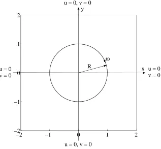
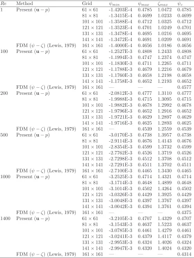
5.1 Flow between rotating circular and fixed square cylinders: Max-imum values of the stream function (ψmax) and vorticity (ζmax),

and values of the stream function on the circular cylinder (ψc)

by the present method and FDM. . . 122

5.2 Natural convection in eccentric circular-circular annulus, sym-metrical flows: the maximum values of the stream function (ψmax)

for two special cases ϕ _{∈ {−}90◦_, ₉₀◦_} _{by the present and some}

other numerical schemes. . . 125

5.3 Natural convection in eccentric circular-circular annulus, unsym-metrical flows: the stream function values at the inner cylinders (ψw) for ε ∈ {0.25, 0.50, 0.75} and ϕ ∈ {−45◦, 0◦, 45◦} by the

(19)

List of Tables xviii

(20)

List of Figures

2.1 1D-IRBF centres on a Cartesian grid line. . . 11

2.2 Local 3-point 1D-IRBF stencil. . . 13

2.3 The plots of basis functions employed in the present studies with

c= 0 anda = 0.2. . . 19

2.4 ODE, N = 51: the effects of the MQ width β on the solution accuracy. . . 21

2.5 ODE, β = 20, N _{∈ {}5, 7, 9, ..., 51_}: the effects of the grid size

h on the system matrix condition (a) and the solution accuracy (b) for the FDM and the present scheme. The matrix condition number grows as O(h−2_{) for the two methods while the solution}

converges as O(h2) for FDM andO(h3.23) for the IRBF method. 22 2.6 Recirculating cavity flow: A schematic diagram of the physical

domain (non-dimensionalised). . . 25

2.7 Recirculating cavity flow, Treatment 2, Re = 100: Variations of u along the vertical centreline (a) and v along the horizontal centreline (b) by the present scheme using a grid of 21_×21 and the exact solution (Shih and Tan, 1989). . . 30

2.8 Lid-driven cavity flow, Re = 1000: Profiles of the u-velocity along the vertical centreline (a) and the v-velocity along the hor-izontal centreline (b) using several grids. Note that curves for the last three grids are indistinguishable and agree well with the benchmark FD results. . . 32

2.9 Lid-driven cavity flow, 129_×129: Profiles of the u-velocity along the vertical centreline and the v-velocity along the horizontal centreline for Re = 100 (a), Re = 400 (b), Re = 1000 (c) and

(21)

List of Figures xx

2.10 Lid-driven cavity flow, 129_×129: Isobaric lines of the flow for

Re= 100 (a), Re= 400 (b), Re= 1000 (c) and Re= 3200 (d). The contour values used here are taken to be the same as those in Abdallah (1987), Botella and Peyret (1998) and Bruneau and Saad (2006). . . 34

2.11 Lid-driven cavity flow, 129 _× 129: Streamlines of the flow for

Re= 100 (a), Re= 400 (b), Re= 1000 (c) and Re= 3200 (d). The contour values used here are taken to be the same as those in Ghia et al. (1982). . . 35

2.12 Lid-driven cavity flow, 129_×129: Iso-vorticity lines of the flow for Re = 100 (a), Re= 400 (b), Re = 1000 (c) and Re = 3200 (d). The contour values used here are taken to be the same as those in Ghia et al. (1982). . . 36

3.1 1D diffusion equation,N _{∈ {}11, 21, . . . , 101_}, ∆t= 0.001,t= 1: The effect of grid sizehon the solution accuracy by the proposed scheme. The solution error behaves apparently as Ne_≈O(h3.4_). ₅₁

3.2 1D diffusion equation, N = 201, ∆t _{∈ {} 1 100,

1 90, . . . ,

1

10}, t =

1: The effect of time step ∆t on the solution accuracy by the proposed scheme. The solution error behaves apparently asNe_≈ O(∆t2_{). . . .} ₅₂

3.3 2D diffusion equation,_{11_×11, 21_×21, . . . , 51_×51_}, ∆t= 0.01,

t = 1: The effect of grid size h on the solution accuracy by the proposed scheme. The solution error behaves apparently as

Ne_≈ O(h3.31). . . 53 3.4 Stokes flow, _{11_×11, 21_×21, . . . , 51_×51_}, ∆t = 10−5_, _t _{= 1:}

The effect of grid sizehon the solution accuracy by the proposed scheme. The solution error behaves asNe _≈O(h3.07_{) and} _Ne_≈

O(h3.1_{) for the velocity (the two indistinguishable lower lines)}

and the pressure, respectively. . . 54

3.5 Shock wave propagation, N _{∈ {}11, 21, . . . , 101_}, Re = 100, ∆t = 10−5_, _t _{= 0}_._{5: The effect of grid size} _h _{on the solution}

accuracy by the proposed scheme. The solution error behaves apparently asNe_≈O(h4.47_{). . . .} ₅₅

3.6 Shock-like solution, N _{∈ {}11, 21, . . . , 101_}, Re _{∈ {}100, 200_}, ∆t = 10−5_, _t _{= 1}_._{7: The effect of grid size} _h _{on the solution}

accuracy by the proposed scheme. The solution error behaves as

(22)

List of Figures xxi

3.7 Torsionally oscillating lid-driven cavity flow: Geometry and bound-ary conditions. . . 62

3.8 Torsionally oscillating lid-driven cavity flow: Profiles ofu-velocity along the vertical centreline during a half cycle of the lid oscil-lation for three values of ω _{∈ {}0.1, 1, 10_} and three values of

Re _{∈ {}100, 400, 1000_}. Times used are t0 = 0, t1 = K/8,

t2 =K/4,t3 = 3K/8,t4 =K/2 andt5 = 3K/4. . . 63

3.9 Torsionally oscillating lid-driven cavity flow: Profiles ofv-velocity along the horizontal centreline during a half cycle of the lid os-cillation for three values of ω _{∈ {}0.1, 1, 10_} and three values of Re _{∈ {}100, 400, 1000_}. Times used are t0 = 0, t1 = K/8,

t2 =K/4,t3 = 3K/8,t4 =K/2 andt5 = 3K/4. . . 65

3.10 Torsionally oscillating lid-driven cavity flow, 65_×65: Evolution of streamlines during a half-cycle of the lid motion atRe= 400 and ω= 1. . . 66

3.11 Torsionally oscillating lid-driven cavity flow, 65_×65: Evolution of streamlines during a half-cycle of the lid motion at Re= 400 and ω= 10. . . 67

4.1 Global 1D-IRBF stencil. . . 75

4.2 Special compact 4-point 1D-IRBF stencils for left and right bound-ary nodes. . . 79

4.3 Unsteady diffusion equation, _{11_×11, 16_×16, . . . , 41_×41_}, ∆t = 10−5_, _t_{= 0}_._{0125 : The effect of grid size} _h _{on the solution}

accuracy for the two present schemes. The solution converges as

O(h2.74_{) for ADI-CIRBF-1 and}_O₍_h4.76_{) for ADI-CIRBF-2. . . .} ₈₆

4.4 Unsteady diffusion equation, ∆t = 10−4_{: The solution accuracy}

(23)

List of Figures xxii

4.5 Unsteady convection-diffusion equation,_{31_×31, 41_×41, . . . , 81_× 81_}, ∆t = 10−4_,_t_{= 1}_._{25: The effect of grid size}_h_{on the solution}

accuracy for the two present schemes. The solution converges as

O(h4.07_{) for ADI-CIRBF-1 and}_O₍_h4.32_{) for ADI-CIRBF-2. . . .} ₈₉

4.6 Unsteady convection-diffusion equation, 81_×81, ∆t = 0.00625: The initial and the computed pulses att= 1.25 by ADI-CIRBF-1 (a) and ADI-CIRBF-2 (b). . . 89

4.7 Unsteady convection-diffusion equation, 81_×81, ∆t = 0.00625: Surface plots of the pulse in the sub-region 1 _≤ x, y _≤ 2 at

t = 1.25 by the analytic solution (a), ADI-CIRBF-1 (b) and ADI-CIRBF-2 (c). . . 90

4.8 Unsteady convection-diffusion equation, 81_×81, ∆t = 0.00625: The solution accuracy of the present schemes and some other techniques against time. . . 92

4.9 Unsteady convection-diffusion equation, 81_×81, ∆t = 0.00625: Contour plots of the pulse in the sub-region 1 _≤ x, y _≤ 2 at

t = 1.25 by the analytic solution (a), standard PR-ADI (b), ADI-CIRBF-1 (c) and ADI-CIRBF-2 (d). . . 94

4.10 Steady convection-diffusion equation,_{11_×11, 16_×16, . . . , 51_× 51_}: The effect of grid sizehon the solution accuracy for the stan-dard PR-ADI and two present schemes. The solution converges asO(h1.94_),_O₍_h3.02_{) and}_O₍_h4.53_{) for PR-ADI, ADI-CIRBF-1 and}

ADI-CIRBF-2, respectively. . . 95

4.11 Steady convection-diffusion equation, 51 _×51: Profiles of the solution u along the vertical and horizontal centrelines by ADI-CIRBF-1 (a)-(b) and ADI-CIRBF-2 (c)-(d). . . 96

5.1 A schematic outline for the problem domain. . . 102

5.2 Special compact 2-point IRBF stencils for the left and right boundary nodes. . . 106

(24)

List of Figures xxiii

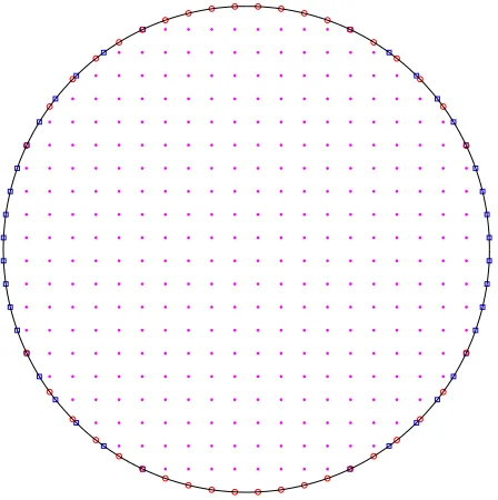
5.4 Poisson equation, circular domain, _{12_×12, 22_×22, . . . , 102_× 102_}: The solution accuracy (a) and the matrix condition num-ber (b) against grid size by FDM and the present method. The solution converges as O(h2.03_{) and}_O₍_h3.17_{) while the matrix}

con-dition grows asO(h−2.52_{) and}_O₍_h−2.46_{) for FDM and the present}

method, respectively. . . 113

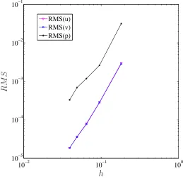
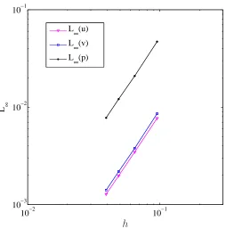
5.5 Taylor-Green vortices, circular domain,_{12_×12, 22_×22, . . . , 52_× 52_}: The solution accuracy of the velocity components and pres-sure against grid size. The solution converges asO(h3.31_),_O₍_h3.29₎

andO(h2.87_{) for}_x_{-component velocity,}_y_{-component velocity and}

pressure, respectively. . . 114

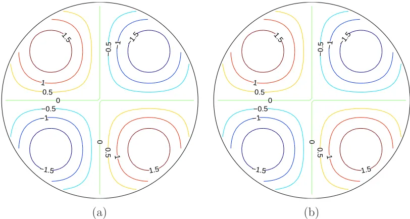
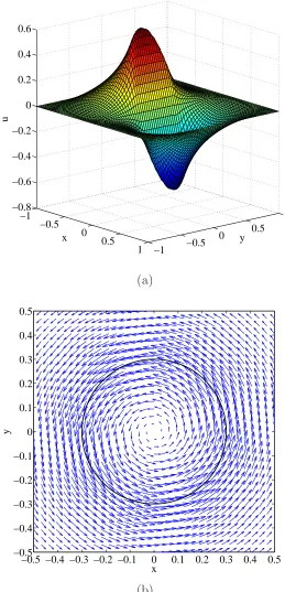
5.6 Taylor-Green vortices, circular domain, 52_×52, ∆t= 0.001: the analytic (a) and computed (b) isolines of the vorticity field at

t= 0.3. . . 115

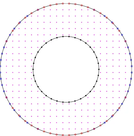
5.7 Taylor-Green vortices, concentric annulus: Computational do-main and its discretisation (Eulerian nodes inside the annulus and on the outer boundary, Lagrangian nodes on the inner bound-ary with a grid of 22_×22). . . 116

5.8 Taylor-Green vortices, concentric annulus, 52_×52, ∆t = 0.001: the analytic (a) and computed (b) isolines of the vorticity field att= 0.3. . . 116

5.9 Taylor-Green vortices, concentric annulus,_{22_×22, 32_×32, . . . , 52_× 52_}: The solution accuracy of the velocity components and pres-sure against grid size. The solution converges asO(h2.02),O(h2.03) andO(h2.02_{) for}_x_{-component velocity,}_y_{-component velocity and}

pressure, respectively. . . 117

5.10 Rotational flow generated by a circular ring rotating about its centre in a fluid filled square cavity, Re = 18, 65_×65, t = 10, ∆t = h/4: Distributions of the x-component velocity (a) and velocity vector (b) over the computational domain. . . 118

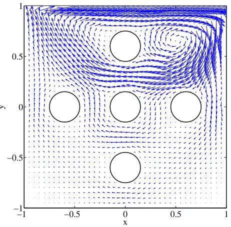
5.11 Lid-driven cavity flow with multiple solid bodies: Geometry and boundary condition. . . 119

(25)

List of Figures xxiv

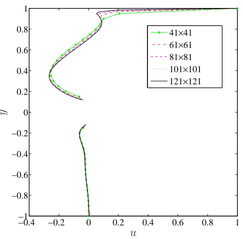
5.13 Lid-driven cavity flow with multiple solid bodies: The effect of the grid size on the u-velocity profile along the diagonal x = y. The curves are discontinuous due to the presence of a circular body on the diagonal around x=y= 0. . . 120

5.14 Flow between a rotating circular and a fixed square cylinder: Geometry and boundary conditions. . . 121

5.15 Flow between a rotating circular and a fixed square cylinder: Streamlines of the flow for several Reynolds numbers using a grid of 131_×131. The contour values used here are taken to be the same as those in Lewis (1979), except those on the circular boundary. . . 123

5.16 Natural convection in eccentric circular-circular annulus: Geom-etry and boundary conditions (a) and distribution of nodes (b) (Eulerian nodes inside the annulus and on the outer boundary, Lagrangian nodes on the inner boundary with a grid of 60_×60). 125

5.17 Natural convection in an eccentric circular-circular annulus, sym-metrical flows: Contour plots for the temperature (a) and stream function (b) fields for ε _{∈ {}0.25, 0.50, 0.75, 0.95_} (from top to bottom) and ϕ = ₋90◦_{. Each plot contains 22 contour lines}

whose levels vary linearly from the minimum to maximum values. 127

5.18 Natural convection in an eccentric circular-circular annulus, sym-metrical flows: Contour plots for the temperature (a) and stream function (b) fields for ε _{∈ {}0.25, 0.50, 0.75, 0.95_} (from top to bottom) and ϕ = 90◦_{. Each plot contains 22 contour lines whose}

levels vary linearly from the minimum to maximum values. . . . 128

5.19 Natural convection in an eccentric circular-circular annulus, un-symmetrical flows: Contour plots for the temperature (a) and stream function (b) fields for ε _{∈ {}0.25, 0.50, 0.75_} (from top to bottom) and ϕ = ₋45◦_{. Each plot contains 22 contour lines}

whose levels vary linearly from the minimum to maximum values. 129

5.20 Natural convection in an eccentric circular-circular annulus, un-symmetrical flows: Contour plots for the temperature (a) and stream function (b) fields for ε_{∈ {}0.25, 0.50, 0.75_}(from top to bottom) and ϕ = 0◦_{. Each plot contains 22 contour lines whose}

(26)

List of Figures xxv

5.21 Natural convection in an eccentric circular-circular annulus, un-symmetrical flows: Contour plots for the temperature (a) and stream function (b) fields forε_{∈ {}0.25, 0.50, 0.75_}(from top to bottom) andϕ = 45◦_{. Each plot contains 22 contour lines whose}

levels vary linearly from the minimum to maximum values. . . . 131

6.1 Configuration with several rigid particles and interstitial fluid domain. . . 136

6.2 Single particle sedimentation: Imaginary particle. . . 141

6.3 Taylor-Green vortices, 151_×151, ∆t= 0.001: Position of the em-bedded circle and the vorticity isolines att= 0.3 for the analytic (a) and present (b) solutions. . . 146

6.4 Taylor-Green vortices, _{31_×31, 61_×61, . . . , 151_×151_}, ∆t = 0.001, t = 0.3: The effect of grid size h on the solution accuracy for the velocity. The solutions converge as aboutO(h2_{) for both}

the present and referential results (Uhlmann, 2005). . . 146

6.5 Induced flow by an oscillating circular cylinder: Configuration of the domain and boundary conditions. . . 147

6.6 Induced flow by an oscillating circular cylinder, 151_×151, ∆t= 0.001: Streamlines of the flow field for different Reynolds num-bers at different times. . . 148

6.7 Induced flow by an oscillating circular cylinder, 151_×151, ∆t= 0.001: The evolution of the drag force for different Reynolds numbers. Re= 100 (dash line) and Re= 800 (solid line). . . 149

6.8 Single particle sedimentation: Schematic view and boundary con-ditions. . . 150

6.9 Single particle sedimentation, 101_×301, ∆t = 0.001: Contours of the vertical velocity at different times. Values of the contour lines: _±{−0.5 :₋0.5 :₋5, 0.5 : 0.5 : 1.5_}. . . 151

6.10 Single particle sedimentation, 101_×301, ∆t= 0.001: Streamlines of the flow field at different times. Values of the contour lines:

±{0.1 : 0.1 : 0.9_}. . . 152

(27)

List of Figures xxvi

6.12 Single particle sedimentation: Time histories of some quanti-ties including the x-coordinate of the particle centre (a), the

y-coordinate of the particle centre (b), the x-component of the translational particle velocity (c), they-component of the transla-tional particle velocity (d), the Reynolds number for the particle (e), and the translational kinetic energy (f). . . 154

6.13 Drafting-kissing-tumbling of two settling particles: Schematic view and boundary conditions. . . 156

6.14 Drafting-kissing-tumbling of two settling particles, 71_×211, ∆t= 6.25_×10−5_{: The evolution of the horizontal (a) and the vertical}

(b) positions of the centre of the two particles. . . 156

6.15 Drafting-kissing-tumbling of two settling particles, 71_×211, ∆t= 6.25_×10−5_{: The evolution of the horizontal (a) and the vertical}

(b) velocities of the two particles. . . 157

6.16 Drafting-kissing-tumbling of two settling particles, 71_×211, ∆t= 6.25_×10−5_{: Contours of the velocity magnitude and the positions}

of particles at different times. . . 158

6.17 Drafting-kissing-tumbling of two settling particles, 71_×211, ∆t= 6.25_×10−5_{: Contours of the vorticity and the positions of}

parti-cles at different times. . . 159

7.1 A sliding bi-periodic frame with crossing and non-crossing sus-pended particles. . . 164

7.2 Illustration of parts of boundaries crossed by particles. . . 174

7.3 Couette flow, 31_×31: Velocity vector field at different shear times.177

7.4 Couette flow, 31_×31: Condition number of the system matrixA. 178

7.5 One-particle problem: A periodic configuration of particles can be modelled by a frame with one single particle for the analysis of the flow. . . 179

7.6 One-particle problem: The angular velocity against the shear time for different particle radii. . . 179

7.7 One-particle problem, R= 0.25, 51_×51, ∆tp = 10−4: Contours

(28)

List of Figures xxvii

7.8 One-particle problem: The bulk shear stress (a) and the bulk normal-stress difference (b) against the shear time for different particle radii. . . 182

7.9 One-particle problem: Relative viscosity against solid-volume fraction. . . 183

7.10 Two-particle problem: Initial configuration of two particles de-pending on D. . . 183

7.11 Two-particle problem, R = 0.12: Contours of vorticity of the flow forD= 0.25. Values of isolines are -0.5:0.25:2.5. . . 184

7.12 Two-particle problem, R = 0.12: Contours of vorticity of the flow forD= 0.025. Values of isolines are -0.5:0.25:2.5. . . 185

7.13 Two-particle problem, R = 0.12: The orbit of the two particle centres forD = 0.025 and D= 0.25. . . 186

7.14 Two-particle problem, R = 0.12: Time-dependent bulk shear stress with respect to the x coordinate of the particle P1 for

D= 0.025 and D= 0.25. . . 186

7.15 Many-particle problem, Np ∈ {1, 2, 3, 4, 5}: Relative viscosity

against solid-volume fraction in dilute suspensions. The first five points on the left correspond to R = 0.05 and the last three points on the right correspond to R = 0.12. The results show that the relative viscosity is independent of particle size in the dilute limit. . . 187

7.16 Many-particle problem: Initial configurations of particles for five-particle problems with R = 0.05 (a) and R= 0.12 (b). . . 188

7.17 Many-particle problem: Vorticity isolines of the flow for five-particle problems with R = 0.05 (a) and R = 0.12 (b) at t = 4. Values of isolines are -0.2:0.2:2 for (a) and -2:0.25:3.5 for (b). . . 189

7.18 Many-particle problem, R = 0.12, Np ∈ {1, 2, 3, 4, 5}: Shear

stress against shear rate at different solid-volume fractions in dilute suspensions. . . 190

7.19 Many-particle problem, R = 0.12, Np ∈ {1, 2, 3, 4, 5}: Flow

(29)

Chapter 1

Introduction

The chapter starts with an overview of particulate suspensions. Conventional numerical methods used for solving fluid flows and fluid-solid systems are then reviewed. Next, we describe radial basis functions that will be utilised to de-velop approximation tools in the proposed computational procedures, which is followed by the motivation and objectives of the present research project. Finally, an outline of the thesis is presented.

1.1

Suspensions

Particulate suspensions widely exist in nature and are commonly produced in in-dustry (Phan-Thien, 2013). Typical examples include paint, inks, biofluids (e.g. blood, mucus and cartilage), cosmetics, food stuff, etc. Particulate suspensions are systems formed by particles suspended in liquids. If the suspending liquid is Newtonian, one speaks of Newtonian suspensions; otherwise, non-Newtonian suspensions. Suspended particles can be rigid bodies, droplets or bubbles. If the suspended particles are identical, one has monodispersed suspensions - oth-erwise, polydispersed suspensions. The particle size also matters too. If the size of suspended particles is sufficiently small, they will undergo their Brow-nian motion and one speaks of colloidal suspensions. If this is not met, one has non-colloidal suspensions. Further details can be found in (Phan-Thien, 2013). In this research project, we are mainly concerned with suspensions of rigid spheres (3D) and circular discs (2D) in a Newtonian fluid (droplets and bubbles will not be considered here).

(30)

1.2 Numerical methods 2

lubrication forces become dominant and special care is needed, particularly for numerical modelling (one needs to maintain meshes/grids between the particle surfaces when the volume fraction is increased). Suspensions are typically char-acterised by (i) the dependence of viscosity on concentration (volume fraction of the solid phase); (ii) non-zero first and second normal stress differences; and (iii) migration of rigid particles from high to low shear regions in an inhomogeneous shear flow such as Poiseuille flow.

1.2

Numerical methods

1.2.1

Simulating fluid flows

From a mathematical point of view, physical processes in nature such as the motion of fluids and heat transfer can be described by a set of partial differential equations (PDEs). These equations are based on the fundamental conservative laws in physics: conservation of mass, conservation of momentum and conser-vation of energy. The governing equations for Newtonian fluid flows are known as the Navier-Stokes equation. Due to the complex nature of the governing equations, analytical solutions cannot be obtained in most cases. Numerical methods have been developed to find an approximate solution. In numerical methods, one needs to discretise the PDEs in both space and time. As a result, a linear/non-linear PDE will be converted into a system of linear/non-linear algebraic equations. Such algebraic systems can then be solved for values of the field variables (e.g. the velocity, pressure and temperature) at discrete points within the computational domains and at all points in the domain by virtue of the assumed interpolation.

(31)

1.2 Numerical methods 3

Recently, the concept of solving PDEs without using a mesh/grid has been introduced. The problem domain is simply discretised by a set of nodes that can be randomly distributed. Like conventional methods, meshless methods have also been developed to deal with the governing equations in their strong form (reproducing kernel particle method (RKPM) (Liu et al., 1995)), weak form (element-free Galerkin (EFG) method (Belytschko et al., 1994), meshless local Petrov-Galerkin (MLPG) (Atluri and Zhu, 1998; Atluri and Shen, 2002; Atluri et al., 2004)) and inverse statement (boundary node method (BNM) (Mukherjee and Mukherjee, 1997; Yang et al., 2011), local boundary integral equation (LBIE) method (Zhu et al., 1998)). Applications of meshless methods for fluid flows have received a great deal of attention because of their economic benefits in dealing with complex geometries such as free surfaces and channels of varying cross-sections.

1.2.2

Modelling fluid-solid systems

If the Navier-Stokes equation governing the motion of a fluid and the Newton-Euler equation governing the motion of solid bodies are solved directly, one speaks of direct numerical simulations (DNSs). Since the solvent is modelled explicitly, DNSs have the ability to deal with any kinds of the suspending liquid and also any shapes and sizes of suspended particles. Based on the fluid-phase solver employed, DNSs can be classified into two categories. In the first cat-egory, a mesh following the movement of the particles, i.e. moving mesh, is used. Methods in this category are usually based on the Arbitrary Lagrangian-Eulerian (ALE) approach, e.g. (Yu et al., 2007, 2004, 2002), (Hu et al., 2001; Hu, 1995; Hu et al., 1992). Finite element methods employed with unstructured meshes have been developed to simulate the motion of a large number of rigid objects in Newtonian and viscoelastic fluids. Nodes on the particle surfaces are allowed to move with the particles, while nodes in the interior of the fluid are smoothly updated by solving a Laplace’s equation. One needs to generate a new mesh when the old one becomes too distorted; the flow field is then projected onto the new mesh. In the second category, a mesh covering the whole domain and independent of the particle movement, i.e. a fixed mesh, is used. Methods in this category include immersed structural potential methods (ISPMs) (Gil et al., 2010), fictitious boundary methods (FBMs) (Turek et al., 2003), immersed boundary methods (IBMs) (Peskin, 2002), sharp interface methods (SIMs) (also called ghost-fluid method) (Liu et al., 2000), virtual boundary methods (VBMs) (Saiki and Biringen, 1996), immersed interface methods (IIMs) (Leveque and Li, 1994), fictitious domain methods (FDMs) (Glowinski et al., 1994), etc. The advantage of the second category over the first one is that it allows a fixed grid to be used and thus eliminating the remeshing procedure.

(32)

1.3 Radial basis functions 4

approach using a fixed frame of reference, the Lagrangian one follows the tra-jectory of individual parts of the material. An advantage in using this approach is that convective terms vanish in Lagrangian formulations and therefore the numerical method employed is simpler. A popular particle-based Lagrangian method is smoothed particle hydrodynamics (SPH) method pioneered by Lucy (1977) and Gingold and Monaghan (1977). Up to date, SPH methods have been improved in terms of both accuracy and stability and they have been ap-plied to many engineering problems successfully (Monaghan, 2005; Randles and Libersky, 1996; Morris et al., 1997; Hashemi et al., 2012). Dilts (1999) proposed a novel method, namely Moving-Least-Squares-Particle Hydrodynamics (ML-SPH), in which the conventional SPH method was newly derived by means of a Galerkin approximation. In this derivation, the SPH interpolant was replaced by the Moving-Least-Squares (MLS) interpolant.

1.3

Radial basis functions

Radial basis functions (RBFs) have emerged as a powerful numerical tool in scattered data approximations and have found applications in various research fields. Kansa (1990a,b) applied RBFs to solve parabolic, hyperbolic and el-liptic PDEs, where the multiquadrics (MQ) function is adopted and used in a global fashion, and the collocation technique is employed to discretise PDEs. Kansa’s method and its variants are hereby referred to as differential/direct RBF (DRBF) methods. The accuracy of MQ is strongly influenced by the so-called shape/width parameter (Carlson and Foley, 1991; Rippa, 1999). In approximating the function and its derivatives, MQ and some other RBFs are known to possess spectral accuracy with an error estimate asO λ√a/h_(Cheng

et al., 2003), where 0< λ < 1, a is the RBF width and h is the characteristic distance between RBFs’ centres. If one approximates the kth derivative, the convergence rate is reduced toO λ√a/h−k_{as shown in Madych (1992). Noting}

(33)

1.4 Motivation and objectives 5

own strengths and weaknesses. For compact local forms, the information about the governing equation or derivatives of the field variable is also included in local approximations, which allows the achievement of sparse system matrices and high levels of accuracy together. This research is concerned with the de-velopment of compact local IRBF approximations for the discretisation of the pressure-velocity formulation in solving viscous flows, fluid-solid interactions and particulate suspensions.

1.4

Motivation and objectives

An understanding of the rheological properties and dynamic behaviours of par-ticulate suspensions is clearly vital in industrial parpar-ticulate-flow processes, e.g. slurries, colloids, fluidised beds, spray drying/cooling in chemical engineering, river sediment in environmental engineering, and rock cuttings in drilling opera-tion in mining and petroleum engineering. Direct numerical simulaopera-tions (DNSs) for the description of microstructures in fluid media, from which bulk proper-ties are derived, have made significant advances over the past twenty years. However, to date, existing DNSs still face major deficiencies with respect to efficiency and accuracy. Given the vastness of industrial processes involving particulate suspensions, any achievement in solving these problems will bring enormous benefits to the industry and consumers. The main objectives of this research are

• To develop computational procedures, which will be both accurate and efficient, for the simulation of heat transfer and steady/unsteady viscous flows.

• To develop accurate and efficient computational procedures for the sim-ulation of steady/unsteady viscous flows in multiply-connected domains that are stationary.

• To develop accurate and efficient computational procedures for the sim-ulation of steady/unsteady viscous flows in multiply-connected domains that vary with time.

• To predict rheological properties of particulate suspensions.

The enhancement of accuracy is achieved through

(34)

1.5 Outline 6

• Using the integral formulation rather than the conventional differential one to construct the RBF approximations (IRBF). A reduction in conver-gence rate in the approximation of derivatives caused by differentiation (Madych, 1992) is avoided in the present integral formulation.

• Constructing the IRBF approximations, where values of the governing equation or derivatives at selected points are also included (compact forms).

The enhancement of efficiency is achieved through

• Using point collocation to discretise the governing equations. No integra-tions are involved in this process.

• Using Cartesian grids rather than finite-element meshes to represent the spatial problem domain. Generating a Cartesian grid is much simpler and easier than generating a finite element mesh.

• Constructing IRBF approximations in a local form, leading to a sparse system matrix.

• Using ADI algorithms of You (2006) to save memory storages and reduce computational costs.

• Converting a multiply-connected domain into a simply-connected domain by means of the direct forcing immersed boundary method.

1.5

Outline

The present thesis has a total of eight chapters including this chapter (Intro-duction). Below are brief descriptions of the remaining chapters.

• In chapter 2, IRBFs are developed for the discretisation of the velocity-pressure formulation on Cartesian grids to simulate 2D steady-state in-compressible viscous flows. A high-order compact local integrated RBF (CLIRBF) approximation scheme and an effective boundary treatment for the pressure variable are proposed. A number of linear and non-linear problems are considered to investigate the performance of the proposed scheme/treatment numerically.

(35)

1.5 Outline 7

• In chapter 4, CLIRBF approximations are employed with the ADI algo-rithm of You (2006) to solve 2D convection-diffusion equation efficiently. Several steady and unsteady problems are considered to verify the present schemes. Results obtained are compared with those by some other ADI schemes.

• In Chapter 5, CLIRBF approximations are employed with the direct forc-ing immersed boundary (DFIB) method to simulate heat transfers and vis-cous flows in multiply-connected domains. The proposed method, namely DFIB-CIRBF, is verified through the solution of several test problems in-cluding Taylor-Green vortices, rotational flow, lid-driven cavity flow with multiple solid bodies, flow between rotating circular and fixed square cylin-ders, and natural convection in an eccentric annulus between two circular cylinders.

• In chapter 6, the present DFIB-CIRBF method is applied for the sim-ulation of fluid-solid systems (the interactions between fluid and rigid particles). Problems considered include Taylor-Green vortices, induced flow by an oscillating circular cylinder, single particle sedimentation and drafting-kissing-tumbling behaviour of two settling particles.

• In chapter 7, the present DFIB-CIRBF method is applied for the sim-ulation of particulate suspensions in a sliding bi-periodic frame and the prediction of their rheological properties numerically. The motion of a liquid and particles are solved in a decoupled manner, where methods for computing the rigid body motion are derived. Results concerning visco-metric behaviour (e.g. viscosity and flow index) are presented.

(36)

Chapter 2

A compact IRBF scheme for

steady-state fluid flows

This chapter is concerned with the development of IRBF method for the simu-lation of 2D steady-state incompressible viscous flows governed by the velocity-pressure formulation on Cartesian grids. Instead of using low-order polynomial interpolants, a high-order compact local IRBF scheme is employed to repre-sent the convection and diffusion terms. Furthermore, an effective boundary treatment for the pressure variable, where Neumann boundary conditions are transformed into Dirichlet ones, is proposed. This transformation is based on global 1D-IRBF approximators using values of the pressure at interior nodes along a grid line and first-order derivative values of the pressure at the two extreme nodes of that grid line. The performance of the proposed scheme is investigated numerically through the solution of several linear (analytic tests including Stokes flows) and non-linear (recirculating cavity flow driven by com-bined shear & body forces and lid-driven cavity flow) problems. Unlike the global 1D-IRBF scheme, the proposed scheme leads to a sparse system ma-trix. Numerical results indicate that (i) the present solutions are more accurate and converge faster with grid refinement in comparison with standard finite-difference results; and (ii) the proposed boundary treatment for the pressure is more effective than conventional direct application of the Neumann boundary condition.

2.1

Introduction

(37)

2.1 Introduction 9

The last two involve less dependent variables than the first one. However, they require some special treatments for the handling of the vorticity boundary condition (theψ₋ω formulation) and the calculation of high-order derivatives including the cross-ones (the ψ formulation). Furthermore, the pressure field needs be resolved, which is generally recognised as a complicated process. For theu₋pformulation, the pressure and velocity fields are obtained directly from the discretised equations and it is straightforward to extend the formulation to 3D problems.

It was reported, e.g. (Roache, 1998; Cheng, 1968; Cyrus and Fulton, 1967), that the use of a conservative form of the governing equation has the ability to give more accurate results than the use of a non-conservative form. In Torrance et al. (1972), through the simulation of a flow in a cavity, it was shown that results by using the conservative equations with first-order accurate interpolants are better than those by using the non-conservative equations with second-order accurate interpolants.

To facilitate a numerical calculation, the spatial domain needs be discretised. Generating a Cartesian grid, which is associated with finite-difference (FD) methods, can be seen to be much more straightforward than generating a finite-element (FE) mesh, which is associated with FE methods and finite-volume (FV) methods.

A fractional-step/projection approach, which is originally suggested by Chorin (1968), is widely applied for the simulation of incompressible viscous flows mod-elled with theu₋pformulation. Variations of this approach have been published in, for example, (Almgren, 1996; Perot, 1993; Bell et al., 1989; Van Kan, 1986; Kim and Moin, 1985). In this study, we will propose a numerical projection method, based on Cartesian grids and a compact local IRBF scheme, for the discretisation of theu₋pformulation in two dimensions. Boundary conditions for the pressure are taken in the form of Dirichlet type, and to do so, we pro-pose a treatment based on global 1D IRBF approximations using values of the pressure at interior nodes along a grid line and first-order derivative values of the pressure at the two extreme nodes of that grid line. The performance of the present method is investigated numerically through the solution of linear and non-linear problems.

(38)

2.2 Mathematical model 10

2.2

Mathematical model

The transient Navier-Stokes equations for an incompressible Newtonian fluid in a domain of interest Ω at the timet can be written in the non-dimensionalised conservative form and in the primitive variables as

∇.u = 0 in Ω, t_≥0, (2.1)

∂u

∂t +∇.(u u) =−∇p+

1

Re∇

2_u₊_fb _{in Ω}_{, t}

≥0, (2.2)

where p, u = (u, v)T, fb = fbx, fby

T

are the static pressure, the fluid velocity vector, and the fluid body force density vector, respectively, defined in the Cartesian x and y coordinate system, the superscript T denotes the transpose;

Re = UL/ν the Reynolds number, in which ν is the kinematic viscosity, L is the characteristic length and U is the characteristic speed of the flow.

For the projection method (Chorin, 1968), the velocity and the pressure vari-ables in the above set of PDEs are solved separately in each iteration. The temporal discretisation of (2.2) with an explicit Euler scheme gives

un₋_un−1

∆t =−∇p

n₊ 1

Re∇

2_un−1

− ∇.(un−1_un−1_{) +}_fn−1

b , (2.3)

where the superscript n denotes the current time level.

An intermediate velocity vector, denoted by u∗,n _{= (}_u∗,n_{, v}∗,n₎T_{, is defined as}

u∗,n₋_un−1

∆t =

1

Re∇

2_un−1

− ∇.(un−1un−1) +f_bn−1. (2.4) This equation, which does not involve the pressure gradient term, can be rewrit-ten as

u∗,n ₌_un−1_{+ ∆}_t

1

Re∇

2_un−1

− ∇.(un−1_un−1_{) +}_fn−1 b

. (2.5)

It is seen that u∗,n _{does not satisfy the continuity equation (2.1). From (2.3)}

and (2.4), one can derive the following equation

un₋_u∗,n

∆t =−∇p

n_. _(2.6)

The Poisson equation for the pressure is then obtained by applying the gradient operator to both sides of (2.6) and forcing un _{to satisfy (2.1)}

∇2_pn₌ 1 ∆t∇·u

(39)

2.3 A brief review of the global 1D-IRBF scheme 11

After solving (2.7), the velocity field at the next time level is calculated through (2.6) as

un=u∗,n

−∆t∇_pn_. _(2.8)

2.3

A brief review of the global 1D-IRBF scheme

Consider the approximation of a univariate functionu(η) and its derivatives up to second order. The second-order derivative of uis decomposed into RBFs

d2_u₍_η₎

dη2 = m

X

i=1

wiGi(η), (2.9)

wheremis the number of RBFs;_{Gi(η)}mi=1the set of RBFs; and{wi}mi=1the set

of weights/coefficients to be found. Approximate representations for the first-order derivative and the function itself are then obtained through integration

du(η)

dη =

m

X

i=1

wiHi(η) +c1, (2.10)

u(η) =

m

X

i=1

wiHi(η) +c1η+c2, (2.11)

where Hi(η) =

R

Gi(η)dη; Hi(η) =

R

Hi(η)dη; and c1 and c2 are the constants

of integration. In the IRBF methods, basis functions are obtained through

η_b1

η₁ η₂ η₃ η_q

η_b2

Figure 2.1: 1D-IRBF centres on a Cartesian grid line.

integration. For several RBFs including the multiquadric function used in the present project, integrated basis functions can be obtained in analytic form and thus equations (2.10) and (2.11) do not require any additional costs when compared to their counterparts of the conventional (differential) RBF methods. Let_{ηi}qi=1 (q=m−2) and {ηb1, ηb2}be a set of interior nodal points and a set

of boundary nodal points, respectively, as shown in Figure 2.1. We choose the set of RBF centres as the set of nodes. Evaluation of (2.11) at the interior and boundary nodes results in

b u b ub

=_H

  cwb1

c2



(40)

2.3 A brief review of the global 1D-IRBF scheme 12

where

b

u= (u1, u2,· · · , uq)T ,

b

ub = (ub1, ub2)T ,

b

w= (w1, w2,· · · , wm)T ,

H=         

H1(η1) · · · Hm(η1) η1 1

H1(η2) · · · Hm(η2) η2 1

..

. . .. ... ... ...

H1(ηq) · · · Hm(ηq) ηq 1

H1(ηb1) · · · Hm(ηb1) ηb1 1

H1(ηb2) · · · Hm(ηb2) ηb2 1

         . (2.13)

The system (2.12), which represents the relation between the RBF space and the physical space and hereafter is called a conversion system, can be solved for the unknown vector of weights (w, cb 1, c2)T by means of the singular value

decomposition (SVD) technique as

  cwb1

c2



=_H−1

b u b ub , (2.14)

where_H−1 is the pseudo-inverse of_H.

Making use of (2.14), (2.10) and (2.9), values of the first and second derivatives of u at the interior and boundary nodes are, respectively, computed as

          du1 dη du2 dη .. . duq dη dub1

dη dub2

dη           =         

H1(η1) · · · Hm(η1) 1 0

H1(η2) · · · Hm(η2) 1 0

... . .. ... ... ...

H1(ηq) · · · Hm(ηq) 1 0

H1(ηb1) · · · Hm(ηb1) 1 0

H1(ηb2) · · · Hm(ηb2) 1 0

        

H−1

b u b ub , (2.15)           

d2_u 1

dη2

d2u2

dη2

.. .

d2_u

q

dη2

d2_u

b1

dη2

d2_u

b2 dη2            =         

G1(η1) · · · Gm(η1) 0 0

G1(η2) · · · Gm(η2) 0 0

... . .. ... ... ...

G1(ηq) · · · Gm(ηq) 0 0

G1(ηb1) · · · Gm(ηb1) 0 0

G1(ηb2) · · · Gm(ηb2) 0 0

        

H−1

b u b ub . (2.16)

These expressions can be rewritten in the following compact form

c du

(41)

2.4 Proposed method 13

and

d d2_u

dη2 =Db2ηbu+bk2η, (2.18)

where the matrices _Db1η and Db2η consist of all but the last two columns of the

product of two matrices on the right-hand side of (2.15) and (2.16), respectively; and bk1η and bk2η are obtained by multiplying the vector ubb with the last two

columns of (2.15) and (2.16) respectively. It is noted that entries ofbk1η andbk2η

are functions of the two boundary values.

It can be seen that derivatives of the functionuat nodes are expressed in terms of nodal values ofu.

2.4

Proposed method

Consider an interior grid point x0 = (x0, y0)T and its associated local 3-point

stencil [η1, η2, η3] (η1 < η2 < η3, η0 ≡ η2) as shown in Figure 2.2, in which η

represents x and y.

η

₁

η

₂

η

₃

Figure 2.2: Local 3-point 1D-IRBF stencil.

2.4.1

A high-order compact local IRBF scheme

Over a local 3-point stencil, we can represent the conversion system as a matrix-vector multiplication

      

u1

u2

u3 d2_u 1

dη2

d2_u 3

dη2       

=

H G

| {z }

C

     

w1

w2

w3

c1

c2

    

(42)

whereui =u(ηi) (i∈ {1, 2, 3}); d

2_u

i

dη2 = d 2_u

dη2(ηi) (i∈ {1, 3});C is the conversion

matrix and _H, _G are submatrices defined as

H=



 HH11((ηη12)) HH22((ηη21)) HH33((ηη21)) ηη21 11

H1(η3) H2(η3) H3(η3) η3 1



, (2.20)

G=

G1(η1) G2(η1) G3(η1) 0 0

G1(η3) G2(η3) G3(η3) 0 0

. (2.21)

Solving (2.19) yields

      w1 w2 w3 c1 c2     

=C

−1        u1 u2 u3 d2_u 1

dη2

d2_u 3 dη2        , (2.22)

which maps the vector of nodal values of the function and of its second derivative to the vector of RBF coefficients including two integration constants. Approxi-mate expressions foruand its derivatives in the physical space are obtained by substituting (2.22) into (2.11), (2.10) and (2.9), respectively.

u(η) = H1(η) H2(η) H3(η) η 1

C−1 d_cub2_u

dη2 !

, (2.23)

du(η)

dη =

H1(η) H2(η) H3(η) 1 0

C−1 d_cbu2_u

dη2 !

, (2.24)

d2_u₍_η₎

dη2 =

G1(η) G2(η) G3(η) 0 0

C−1 d_cbu2_u

dη2 !

, (2.25)

where η1 ≤ η ≤ η3; ub= (u1, u2, u3)T and dc

2_u

dη2 = (d 2_u₁

dη2 ,d 2_u₃

dη2 )T. The above three

equations can be rewritten in the form

u(η) =

3

X

i=1

ϕi(η)ui+ϕ4(η)

d2_u 1

dη2 +ϕ5(η)

d2_u 3

dη2 , (2.26)

du(η)

dη =

3

X

i=1

dϕi(η)

dη ui+

dϕ4(η)

dη d2_u

1

dη2 +

dϕ5(η)

dη d2_u

3

dη2 , (2.27)

d2_u₍_η₎

dη2 = 3

X

i=1

d2_ϕ i(η)

dη2 ui+

d2_ϕ 4(η)

dη2

d2_u 1

dη2 +

d2_ϕ 5(η)

dη2

d2_u 3

dη2 , (2.28)

where_{ϕi(η)}5i=1 is the set of IRBFs in the physical space. It can be seen from

(43)

not only nodal function values but also nodal second-derivative values.

The present compact local 3-point IRBF scheme is utilised to represent the variations of the velocity components, the intermediate velocity components and the pressure in (2.3)-(2.8).

2.4.2

Two boundary treatments for the pressure

In order to solve the pressure Poisson equation (2.7), a boundary condition for the pressure is required. On the non-slip boundaries, from the momentum equation (2.2), one can derive the Neumann boundary condition for the pressure as ∂pn b ∂x = 1 Re

∂2_un−1 b

∂x2 +

∂2_un−1 b

∂y2

−

∂(un−1 b u

n−1 b )

∂x +

∂(vn−1 b u

n−1 b )

∂y

+fbnx−1

= u

∗,n b −unb

∆t , (2.29)

∂pn b ∂y = 1 Re

∂2_vn−1 b

∂x2 +

∂2_vn−1 b

∂y2

−

∂(un_b−1v_bn−1)

∂x +

∂(vn_b−1vn_b−1)

∂y

+fbny−1

= v

∗,n b −vbn

∆t . (2.30)

In what follows, we will describe an implementation of the Neumann boundary condition in the context of IRBFs (Treatment 1), and present a new treatment, which transforms the Neumann boundary condition into the Dirichlet one, and its detailed implementation (Treatment 2).

Treatment 1

The boundary condition for the pressure is imposed in the Neumann form. Assume that η1 is a boundary node (i.e. ηb1 ≡ η1). At the current time level

n, one can calculate the value of ∂p/∂η at ηb1 through (2.29) and (2.30). We

modify the conversion system (2.19) as

       pn 1 pn 2 pn 3 ∂pn b1 ∂η ∂2_pn−1

3 ∂η2        = 

 H_H

G         wn 1

w2n

wn 3 cn 1 cn 2     

(44)

where∂pn

b1/∂ηand ∂2pn3−1/∂η2 are known values;H is defined as in (2.20); and H= H1(ηb1) H2(ηb1) H3(ηb1) 1 0 , (2.32) G= G1(η3) G2(η3) G3(η3) 0 0

. (2.33)

Equation (2.31) leads to

      wn 1 wn 2 wn 3 cn 1 cn 2      = 

 H_H

G   −1        pn 1 pn 2 pn 3 ∂pn b1 ∂η ∂2_pn−1

3 ∂η2        . (2.34)

It can be seen that there are two unknowns over the stencil associated with

η0 ≡ η2, namely pb1n and pn2. As a result, apart from collocating (2.7) at η2 for

the unknown pn

2, one also needs to collocate (2.7) at ηb1 for the unknown pnb1.

Values of the second derivative of p at ηb1 and η2 at the current time level are

thus computed as

∂2_pn b1

∂η2

∂2_pn

2

∂η2 !

=

G1(ηb1) · · · Gm(ηb1) ηb1 1

G1(η2) · · · Gm(η2) η2 1



 H_H

G   −1        pn 1 pn 2 pn 3 ∂pn b1 ∂η ∂2_pn−1

3 ∂η2        . (2.35) Treatment 2

The boundary condition for the pressure is imposed in the Dirichlet form. The process of deriving Dirichlet boundary conditions for the pressure is based on the global 1D-IRBF approximation scheme, i.e. (2.9)-(2.11), using the previous values of the pressure at interior nodes along a grid line and the current first-order derivative values of the pressure at the two extreme nodes of that grid line (Thai-Quang et al., 2011).

Consider a grid lineη and letm be the number of nodes on the grid line. From (2.29)-(2.30), one can obtain derivative values of the pressure at the two extreme nodes, i.e. ∂pn_b1/∂η and ∂pn_b2/∂η. We modify the conversion system (2.12) as

  

b pn−1

∂pn b1 ∂η ∂pn b2 ∂η   = H H 

 wb

n

cn1

cn 2



(45)

where the left-hand side is a known vector

b

pn−1 ₌ _pn−1

1 , pn2−1,· · · , pnq−1

T

, (q =m₋2), b

wn= (w₁n, w₂n,_{· · ·} , wn_m)T ,

H=     

H1(η1) · · · Hm(η1) η1 1

H1(η2) · · · Hm(η2) η2 1

... . .. ... ... ...

H1(ηq) · · · Hm(ηq) ηq 1

   

, (2.37)

H=

H1(ηb1) · · · Hm(ηb1) 1 0

H1(ηb2) · · · Hm(ηb2) 1 0

. (2.38)

Values of the pressure at the two extreme nodes at the current time level are then estimated by collocating (2.11) at ηb1 and ηb2 and making use of (2.36)

pn b1 pn b2 =

H1(ηb1) · · · Hm(ηb1) ηb1 1

H1(ηb2) · · · Hm(ηb2) ηb2 1

H H −1    b pn−1

∂pn b1 ∂η ∂pn b2 ∂η  

. (2.39)

We use these known values as Dirichlet boundary conditions in solving the pressure Poisson equation (2.7).

2.4.3