Linked simulation-optimization based methodologies for unknown groundwater pollutant source identification in managed and unmanaged contaminated sites

Full text

(1)ResearchOnline@JCU. This file is part of the following reference:. Jha, Manish Kumar (2012) Linked simulationoptimization based methodologies for unknown groundwater pollutant source identification in managed and unmanaged contaminated sites. PhD thesis, James Cook University.. Access to this file is available from:. http://researchonline.jcu.edu.au/40015/ The author has certified to JCU that they have made a reasonable effort to gain permission and acknowledge the owner of any third party copyright material included in this document. If you believe that this is not the case, please contact [email protected] and quote http://researchonline.jcu.edu.au/40015/.

(2) Linked Simulation-Optimization Based Methodologies for Unknown Groundwater Pollutant Source Identification in Managed and Unmanaged Contaminated Sites Thesis submitted by Manish Kumar Jha, B.Tech, M.Tech. for the degree of Doctor of Philosophy (PhD) in the School of Engineering and Physical Sciences James Cook University November 2012.

(3) STATEMENT OF ACCESS. I, the undersigned, author of this work, understand that James Cook University will make this thesis available for use within the University Library and, via the Australian Digital Theses network, for use elsewhere.. I understand that, as an unpublished work, a thesis has significant protection under the Copyright Act and I wish this work to be embargoed until March 2013.. After which date I do not wish to place any further restriction on access to this work.. Signature. Date. i.

(4) STATEMENT OF SOURCES DECLARATION. I herewith declare that I have produced this thesis without the prohibited assistance of third parties and without making use of aids other than those specified; notions taken over directly or indirectly from other sources have been identified as such. This thesis has not previously been presented in identical or similar form to any other Australian or foreign examination board.. Signature. Date. ii.

(5) ELECTRONIC COPY. I, the undersigned, the author of this work, declare that the electronic copy of this thesis provided to James Cook University Library is an accurate copy of the print thesis submitted.. Signature. Date. iii.

(6) STATEMENT OF CONTRIBUTION OF OTHERS. Financial contribution towards this PhD project was received from:. 1. Scholarship from Cooperative Research Centre for Contamination Assessment and Remediation of the Environment (CRC CARE), Salisbury South, SA 5106, Australia.. 2. School of Engineering and Physical Sciences, James Cook University, Graduate Research Scheme funding for travel and equipment in 2010.. Apart from the financial assistance, the following have contributed to this PhD project as specified hereunder:. • Dr. Bithin Datta : Dr. Datta supervised the entire PhD project and helped conceptualize the problem, suggested several ways of solving it and provided insights to the tools and technologies used in this thesis. • Department of Environment and Resource Management, Queensland : Provided field data for validation of some of the methodologies developed in this thesis.. iv.

(7) Acknowledgements. Foremost, I am deeply indebted to my supervisor Dr.. Bithin. Datta, whose patience, kindness and vast academic experience, have been invaluable to me. Without his continuous and unconditional support, this thesis would not have been possible. I am also thankful to CRC CARE for generously funding my research and providing substantial support for attending several conferences during the course of my study. I must also thank the School of Engineering and Physical Sciences at James Cook University for providing excellent infrastructure and a collaborative work environment. My colleagues at James Cook University, especially the PhD candidates in Engineering, have been my support network throughout the tenure of my PhD candidature. I am grateful to all my colleagues who made my stay at JCU a lot more enjoyable and fun-filled..

(8) Abstract. Groundwater is the primary source for irrigation and drinking in many parts of the world. Anthropogenic activities such as mining; large scale production, storage and transport of various chemicals; improper waste management practices; and unsustainable intensive agricultural practices have resulted in the contamination of many groundwater aquifers. The identification of the exact location and release history of contributing sources, which are often unknown, is very important in planning effective remediation measures as well as in determining the liability on the polluter. Contamination of ground water aquifers may be caused by a combination of pollutant sources varying in time of release, flux and location. In situations where they are unknown, location and release histories have to be estimated by inversion. Inversion of the equations governing flow and transport over time and space is an ill-posed problem. Estimation. of. unknown. groundwater. pollutant. source. characteristics from measured pollutant concentrations at several monitoring locations is generally an ill-posed and sometimes non-unique inverse problem. Linked simulation-optimization based methodologies have evolved as effective tools capable of solving this problem..

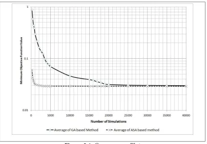
(9) One. of. the. important. issues. in. estimation. of. unknown. contamination sources is the release history reconstruction. It is generally assumed that reliable information on potential source locations and their time of activity is available from background studies of anthropogenic activities on a contaminated site. In such cases, only the release history of the pollutant sources is unknown. Some of the main limitations in accurate source characterization are: 1. Sparsity of concentration measurement data. 2. Inefficient monitoring network for concentration measurements. 3. Difficulty in establishing the time of pollutant source activity initiation. 4. Applicability of optimal source characterization to distributed sources. 5. Problems associated with achieving a global optimal solution efficiently. In order to address some of these limitations, initially a linked simulation-optimization model for optimal source characterization is developed using adaptive simulated annealing (ASA) as the optimization algorithm.. Performance of the ASA based. methodology was compared with a source characterization method using genetic algorithm (GA) for optimization, in terms of their ability to handle uncertainties and efficiency of convergence. Using illustrative aquifer examples, it was shown that ASA converges faster and produces better results even with erroneous measurement.

(10) data and with uncertainties in hydraulic conductivity and porosity. A more complex scenario exists when no reliable information is available on the potential location or initial time of activity of sources.. Apart from this, the frequency of measurement at. monitoring wells may not be uniform and some measurements might be missing in practical situations. A methodology is developed to generate initial estimates of source characteristics such as source location and to estimate the initial time of activity from pollutant concentration measurements obtained from a single location where the contamination was first detected. dynamic time warping (DTW) distance is used to minimize errors in estimation of source characteristics arising from improper alignment of estimated and observed concentration data on the temporal axis. Performance of this methodology is evaluated using data obtained from both an illustrative site and an actual contaminated site. Based on these estimates, a methodology is developed to design a monitoring network to generate concentration measurement information aimed at obtaining more reliable estimates of source characteristics.. This methodology is implemented for a real. contaminated site and it was found that the use of developed methodology results in reliable estimates of source characteristics with a far lesser number of monitoring wells. The source characterization methodology is then extended for estimation of release history of distributed pollutant sources in a realistic scenario.. Distributed sources in an abandoned.

(11) mine site were considered for this purpose.. A conceptual. flow model is developed and calibrated for an abandoned mine site in South-East Queensland.. Various illustrative scenarios of. contamination are considered for evaluating the performance of this developed methodology.. It was shown that the developed. methodology is potentially applicable for estimation of distributed source characteristics. When. management. measures. are. implemented. to. control. contamination in a groundwater aquifer, measured concentration values are the resultant effect of natural transport and control measures.. This can produce incorrect estimates for source. characteristics. The methodology for release history reconstruction can be applied to managed contaminated sites by incorporating the proposed management strategy into the groundwater flow or transport model. This is illustrated by incorporating contamination management strategies already in place into the groundwater flow and transport model for an abandoned mine site with some degree of existing control measures..

(12) Contents List of Figures. xv. List of Tables. xviii. List of Symbols and Abbreviations 1. 2. xx. Introduction. 1. 1.1. Unknown Groundwater Pollutant Source Characterisation . . .. 3. 1.2. Linked Simulation-Optimization Approach . . . . . . . . . . . .. 5. 1.3. Research Objectives . . . . . . . . . . . . . . . . . . . . . . . . . .. 6. 1.4. Organization of the Thesis . . . . . . . . . . . . . . . . . . . . . .. 8. Review of Literature. 10. 2.1. 10. Unknown Groundwater Pollutant Source Characterisation . . . 2.1.1. Linked Unknown. Simulation-Optimization Groundwater. Approach. Contaminant. of. Source. Characterisation . . . . . . . . . . . . . . . . . . . . . . . 2.2. 2.3. 12. Monitoring Network Design for Unknown Groundwater Contaminant Source Characterisation . . . . . . . . . . . . . . .. 18. Relevant Tools and Techniques . . . . . . . . . . . . . . . . . . .. 24. 2.3.1. Flow and Transport Modelling . . . . . . . . . . . . . . .. 24. 2.3.2. Techniques for Parameter Uncertainty Representation .. 26. x.

(13) 2.4 3. 2.3.3. Optimization Algorithms . . . . . . . . . . . . . . . . . .. 27. 2.3.4. Techniques for Pattern Recognition and Classification .. 30. Motivation for this Study . . . . . . . . . . . . . . . . . . . . . .. 31. Three-Dimensional. Groundwater. Contamination. Source. Identification Using Adaptive Simulated Annealing. 33. 3.1. Methodology . . . . . . . . . . . . . . . . . . . . . . . . . . . . .. 37. 3.2. Simulation of Groundwater Flow and Transport . . . . . . . . .. 38. 3.2.1. Mathematical Representation of Groundwater Flow and Transport . . . . . . . . . . . . . . . . . . . . . . . . . . .. 3.2.2. 3.3. 3.4. 38. Numerical Solution of Groundwater Flow and Transport Equations . . . . . . . . . . . . . . . . . . . . . . . . . . .. 42. 3.2.2.1. MODFLOW . . . . . . . . . . . . . . . . . . . .. 43. 3.2.2.2. MT3DMS . . . . . . . . . . . . . . . . . . . . . .. 44. 3.2.3. Formulation of the Optimization Problem . . . . . . . .. 44. 3.2.4. Optimization Algorithms . . . . . . . . . . . . . . . . . .. 46. 3.2.5. Suitability and Sensitivity of Adaptive Simulated Annealing . . . . . . . . . . . . . . . . . . . . . . . . . . .. 47. Performance Evaluation . . . . . . . . . . . . . . . . . . . . . . .. 49. 3.3.1. Simulating Errors in Concentration Measurement Data .. 50. 3.3.2. Incorporating Uncertainty in Hydrogeologic Parameters. 51. 3.3.3. Performance Evaluation Criteria . . . . . . . . . . . . . .. 52. 3.3.4. Incorporation of Different Concentration Monitoring Scenarios . . . . . . . . . . . . . . . . . . . . . . . . . . . .. 54. Discussion of Solution Results . . . . . . . . . . . . . . . . . . .. 55. 3.4.1. 55. Study Area . . . . . . . . . . . . . . . . . . . . . . . . . .. xi.

(14) 3.4.2. Source Flux Magnitude Estimation with Error Free Data. 58. 3.4.3. Source Flux Magnitude Estimation with Erroneous Data. 60. 3.4.4. Source Flux Magnitude Estimation with Uncertainty in Hydrogeologic Parameters . . . . . . . . . . . . . . . . .. 62. Effects of Monitoring Network . . . . . . . . . . . . . . .. 66. Conclusion . . . . . . . . . . . . . . . . . . . . . . . . . . . . . . .. 70. 3.4.5 3.5 4. Methodology for Initial Estimation of Unknown Pollutant Source Characteristics and Design of Monitoring Network 4.1. Preliminary Estimation of Unknown Groundwater Pollutant Source Characteristics . . . . . . . . . . . . . . . . . . . . . . . . 4.1.1. 4.1.2. 4.1.3. 4.3 5. 75. Pattern Comparison using Dynamic Time Warping Distance . . . . . . . . . . . . . . . . . . . . . . . . . . . .. 4.2. 72. 79. Pattern Comparison using DTW Distance to Estimate the Time of First Activity of Unknown Pollutant Source. 81. Initial Source Characteristics Estimation . . . . . . . . .. 85. Monitoring Network Design for Efficient Unknown Pollutant Source Characterisation . . . . . . . . . . . . . . . . . . . . . . .. 90. Conclusion . . . . . . . . . . . . . . . . . . . . . . . . . . . . . . .. 91. Performance Evaluation of Methodology for Initial Estimation of Unknown Pollutant Source Characteristics and Design of Monitoring Network 5.1. 93. Performance Evaluation Criteria for Initial Estimation of Unknown Pollutant Source Characteristics . . . . . . . . . . . .. xii. 93.

(15) 5.1.1. 5.2. 5.3. Performance. Evaluation. Criteria. for. Monitoring. Network Design . . . . . . . . . . . . . . . . . . . . . . .. 94. Results and Discussion . . . . . . . . . . . . . . . . . . . . . . . .. 95. 5.2.1. Study Area . . . . . . . . . . . . . . . . . . . . . . . . . .. 95. 5.2.2. Initial Estimation of Source Characteristics . . . . . . . .. 96. 5.2.3. Monitoring Network Design . . . . . . . . . . . . . . . . 102. Application to a Contaminated Aquifer . . . . . . . . . . . . . . 105 5.3.1. Site Description . . . . . . . . . . . . . . . . . . . . . . . . 105. 5.3.2. Groundwater Flow Model and its Calibration . . . . . . 107 5.3.2.1. Boundary Conditions . . . . . . . . . . . . . . . 109. 5.3.2.2. Sources and Sinks . . . . . . . . . . . . . . . . . 110. 5.3.2.3. Model Calibration . . . . . . . . . . . . . . . . . 110. 5.3.3. Groundwater Transport Model . . . . . . . . . . . . . . . 114. 5.3.4. Performance. Evaluation. of. Initial. Estimation. of. Unknown Pollutant Source Characteristics . . . . . . . . 118 5.3.5 5.4 6. of. Release. History. Distributed. Sources. incorporating. Interactions 6.1. 6.2. 120. Conclusion . . . . . . . . . . . . . . . . . . . . . . . . . . . . . . . 122. Application to. Performance Evaluation of Monitoring Network Design. Estimation. Methodology. Surface-Groundwater 124. Site Description . . . . . . . . . . . . . . . . . . . . . . . . . . . . 126 6.1.1. Topography and Climate . . . . . . . . . . . . . . . . . . 127. 6.1.2. Hydrology . . . . . . . . . . . . . . . . . . . . . . . . . . . 127. Numerical Groundwater Flow Modelling . . . . . . . . . . . . . 129 6.2.1. Geology and Hydrogeology . . . . . . . . . . . . . . . . . 132. xiii.

(16) 6.2.2. Model Layers . . . . . . . . . . . . . . . . . . . . . . . . . 134. 6.2.3. Hydrogeological Properties . . . . . . . . . . . . . . . . . 135. 6.2.4. Sources, Sinks and Boundary Conditions . . . . . . . . . 135. 6.2.5. Model Calibration . . . . . . . . . . . . . . . . . . . . . . 136. 6.3. Transport Model . . . . . . . . . . . . . . . . . . . . . . . . . . . 145. 6.4. Performance Evaluation of Release History Reconstruction Methodology . . . . . . . . . . . . . . . . . . . . . . . . . . . . . 152. 6.5 7. Conclusion . . . . . . . . . . . . . . . . . . . . . . . . . . . . . . . 154. Conclusions. 155. References. 159. xiv.

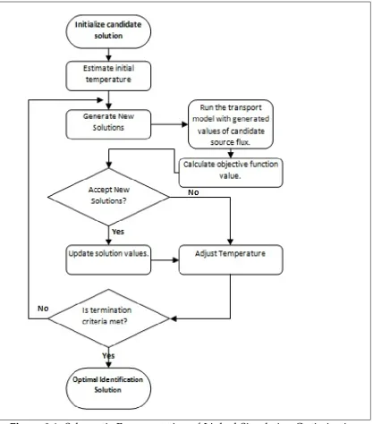
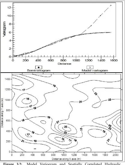
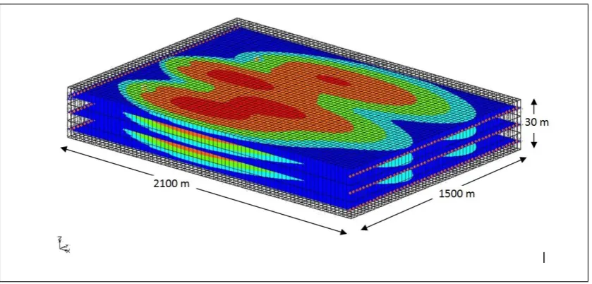
(17) List of Figures 3.1. Schematic Representation of Linked Simulation-Optimization Model using Adaptive Simulated Annealing . . . . . . . . . . .. 3.2. Model. Variogram. and. Spatially. Correlated. 39. Hydraulic. Conductivity Values Generated for the First Layer . . . . . . . .. 53. 3.3. Illustrative Study Area . . . . . . . . . . . . . . . . . . . . . . . .. 55. 3.4. Top View of Study Area Showing Sources and Monitoring Locations . . . . . . . . . . . . . . . . . . . . . . . . . . . . . . . .. 56. 3.5. Estimated Release History with Error Free Data . . . . . . . . .. 59. 3.6. Convergence Plot . . . . . . . . . . . . . . . . . . . . . . . . . . .. 61. 3.7. Reconstructed Release Histories using the Competing Methods. 63. 3.8. Various Monitoring Networks . . . . . . . . . . . . . . . . . . . .. 67. 3.9. Characteristic Curves of Wells on Chosen Monitoring Networks. 68. 3.10 Source. Release. History. Reconstruction. using. Different. Monitoring Networks . . . . . . . . . . . . . . . . . . . . . . . .. 69. 4.1. Illustrative Example of Initial Pollutant Detection . . . . . . . .. 74. 4.2. Breakthrough Curve at a Monitoring Location . . . . . . . . . .. 76. 4.3. Illustrative Example of Pattern Comparison using Dynamic. 4.4. Time Warping . . . . . . . . . . . . . . . . . . . . . . . . . . . . .. 82. Computed DTW Distance over Time . . . . . . . . . . . . . . . .. 84. xv.

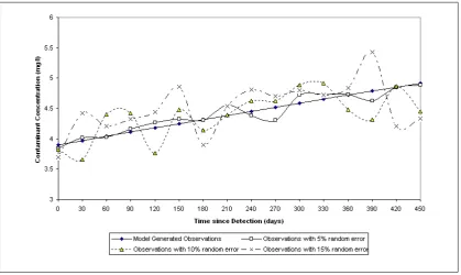
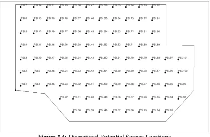
(18) 4.5. Effects of Approximation of Source Flux Magnitudes on Breakthrough Curve . . . . . . . . . . . . . . . . . . . . . . . . .. 87. 4.6. Flowchart Showing the Steps in Initial Estimation . . . . . . . .. 89. 5.1. Illustrative Study Area . . . . . . . . . . . . . . . . . . . . . . . .. 95. 5.2. Actual Release History of the Source . . . . . . . . . . . . . . . .. 98. 5.3. Model Generated Observation Sequences with Synthetic Errors. 98. 5.4. Discretized Potential Source Locations . . . . . . . . . . . . . . . 100. 5.5. Potential Monitoring Locations . . . . . . . . . . . . . . . . . . . 102. 5.6. Estimated Release History . . . . . . . . . . . . . . . . . . . . . . 104. 5.7. Location of the Study Area within Upper Macquarie Groundwater Model . . . . . . . . . . . . . . . . . . . . . . . . . 105. 5.8. Extent of Study Area and Contaminated Area, Elevation Profile and Location of Monitoring Wells . . . . . . . . . . . . . . . . . 107. 5.9. Layers of the Developed Conceptual Model . . . . . . . . . . . . 108. 5.10 Model of the Study Area . . . . . . . . . . . . . . . . . . . . . . . 109 5.11 Components of a Calibration Target Box Plot . . . . . . . . . . . 111 5.12 Calibration Results of Groundwater Flow Model . . . . . . . . . 113 5.13 Estimated vs Observed Heads after Calibration . . . . . . . . . 114 5.14 Simulated Heads in Layer 1 . . . . . . . . . . . . . . . . . . . . . 115 5.15 Simulated Heads in Layer 2 . . . . . . . . . . . . . . . . . . . . . 116 5.16 Simulated Heads in Layer 3 . . . . . . . . . . . . . . . . . . . . . 117 6.1. Topographical Features of the Study Area. Adapted from: Wels et al. (2006) . . . . . . . . . . . . . . . . . . . . . . . . . . . . . . . 128. 6.2. The Don and Dee River Groundwater Management Unit Boundaries. Adapted from: Government of Queensland (2011) 130. xvi.

(19) 6.3. Historical Catchment Boundaries. Adapted from: Unger et al. (2003) . . . . . . . . . . . . . . . . . . . . . . . . . . . . . . . . . . 131. 6.4. Geology of the Mine Site Adapted from: Taube (1986) . . . . . . 133. 6.5. Top Elevation Contour Map and MODFLOW Boundary Conditions in Layer 1 . . . . . . . . . . . . . . . . . . . . . . . . . 137. 6.6. Top Elevation Contour Map and MODFLOW Boundary Conditions in Layer 2 . . . . . . . . . . . . . . . . . . . . . . . . . 138. 6.7. Top Elevation Contour Map and MODFLOW Boundary Conditions in Layer 3 . . . . . . . . . . . . . . . . . . . . . . . . . 139. 6.8. Top Elevation Contour Map and MODFLOW Boundary Conditions in Layer 4 . . . . . . . . . . . . . . . . . . . . . . . . . 140. 6.9. Estimated vs Observed Heads after Calibration . . . . . . . . . 142. 6.10 Calibrated Groundwater Model of the Study Area . . . . . . . . 143 6.11 Recharge Rates for Various Recharge Zones in the Study Area . 146 6.12 Simulated Heads in Layer 1 . . . . . . . . . . . . . . . . . . . . . 147 6.13 Simulated Heads in Layer 2 . . . . . . . . . . . . . . . . . . . . . 148 6.14 Simulated Heads in Layer 3 . . . . . . . . . . . . . . . . . . . . . 149 6.15 Simulated Heads in Layer 4 . . . . . . . . . . . . . . . . . . . . . 150 6.16 Estimated Source Concentrations and Convergence Profile for Various Error Levels . . . . . . . . . . . . . . . . . . . . . . . . . 153. xvii.

(20) List of Tables 3.1. Model Parameters . . . . . . . . . . . . . . . . . . . . . . . . . . .. 57. 3.2. Actual Source Fluxes . . . . . . . . . . . . . . . . . . . . . . . . .. 58. 3.3. Parameters used in Optimization Algorithms . . . . . . . . . . .. 60. 3.4. Normalized Absolute Error of Estimation . . . . . . . . . . . . .. 62. 3.5. Performance Evaluation for Uncertainty in Hydrogeologic Parameters . . . . . . . . . . . . . . . . . . . . . . . . . . . . . . .. 65. 5.1. Model Parameters . . . . . . . . . . . . . . . . . . . . . . . . . . .. 96. 5.2. Actual Source Characteristics . . . . . . . . . . . . . . . . . . . .. 97. 5.3. Estimation of Preliminary Source Characteristics using Error Free Observed Data . . . . . . . . . . . . . . . . . . . . . . . . . . 101. 5.4. Monitoring Locations Chosen in the Optimal Monitoring Network and Arbitrary Monitoring Networks for Comparison. 103. 5.5. Extraction Wells in the Study Area . . . . . . . . . . . . . . . . . 110. 5.6. Parameters Used for Flow and Transport Model of BTEX Affected Study Area . . . . . . . . . . . . . . . . . . . . . . . . . 118. 5.7. Initial Estimates of Source Characteristics . . . . . . . . . . . . . 120. 5.8. Source. Characteristics. Obtained. using. Linked. Simulation-Optimization Method . . . . . . . . . . . . . . . . . . 122. xviii.

(21) 6.1. Parameters Used for Flow and Transport Model of the Study Area . . . . . . . . . . . . . . . . . . . . . . . . . . . . . . . . . . . 141. 6.2. Observed and Estimated Values of Hydraulic Head at Various Monitoring Locations . . . . . . . . . . . . . . . . . . . . . . . . . 144. 6.3. Actual Source Concentrations . . . . . . . . . . . . . . . . . . . . 151. xix.

(22) Kij. The hydraulic conductivity tensor (LT −1 ). Ss. The specific storage of the porous media. ( L −1 ) Sud. Partial List of. A uniform random number between -1 and +1. Symbols and. ASA. Adaptive Simulated Annealing. C. Concentration of pollutants dissolved in groundwater, (ML−3 ). Abbreviations. DERM. Department of Environmental Resources Management, Govt.. ∆x. Finite. Difference. grid. spacing. Australia.. in. x-direction ∆y. DTW. Dynamic Time Warping. GA. Genetic Algorithm. GMU. Groundwater Management Unit. h. Potentiomentric Head (L). dimensionless. NAEE. Normalized absolute error of estimation. Seepage or linear pore water velocity,. NSW. New South Wales, Australia. SA. Simulated Annealing. SRTM. Shuttle Radar Topography Mission. t. The time (T). UNEP. United Nations Environment Programme. Finite. Difference. grid. spacing. in. y-direction ∆z. of Queensland,. Finite. Difference. grid. spacing. in. z-direction θ. ϑi. Porosity. of. the. porous. medium,. (LT −1 ) Cns. Simulated concentration. C pert. Perturbed. contaminant. concentration. value Dij. Hydrodynamic. dispersion. coefficient,. (L2 T −1 ). xx.

(23) Chapter 1. Introduction Groundwater resources are susceptible to contamination from pollutants generated by anthropogenic agricultural and industrial activities.. Often,. when the contamination is first detected, little is known about the various characteristics of the pollutant source. This study presents methodologies for unknown groundwater pollutant source characterisation using linked simulation-optimization approach. The performance of these methodologies are evaluated for practical scenarios of point and distributed sources of groundwater pollution. Water is essential to support life and for the preservation of environment. Due to growing populations of human beings and associated increase in anthropogenic activities such as agriculture and industrialisation, water demand has risen sharply. According to the recent estimates published by UNEP, global water consumption has tripled over the past 50 years (Gaddis et al., 2012).. In many parts of the world, groundwater is the primary. source for irrigation and drinking water supply. With increasing dependency of some regions on groundwater, global groundwater abstraction rate has more than doubled between 1960 and 2000 (Wada et al., 2010). Total global groundwater abstraction was estimated to be about 600-700 km3 yr −1 in 2003. In the same year, groundwater was estimated to meet at least 50% of potable. 1.

(24) water supplies; 40% of the demand from those industries that do not use mains water, and 20% of water use in irrigated agriculture. Dependence on groundwater is particularly becoming prominent in expanding urban communities. It has been estimated that about 1500 million urban dwellers worldwide depend on well, borehole and spring sources (Foster and Chilton, 2003). Given the importance of groundwater in meeting current global water demand, sustainability of groundwater resources is vital for ensuring long-term water security.. A major constraint to the sustainability of. groundwater resources is quality deterioration.. Among various reasons. for groundwater quality degradation, anthropogenic contamination and salination of groundwater are the most important (Morris et al., 2003). Groundwater resources are polluted mainly because of pollutant streams generated by rapidly increasing industrial activities and use of chemicals in agriculture. Some of the more severe incidents of groundwater pollution with large plumes of high concentration pollutants are associated with industrial point sources from major accidental spillage or casual discharge in highly vulnerable areas (Foster and Chilton, 2003). The realization of increasing vulnerability of groundwater resources to pollution has necessitated development of efficient techniques for prevention, detection and remediation of contaminated groundwater aquifers. Contamination of groundwater resources can often remain undetected for significant periods of time. In order to develop methodologies for effective and economical remediation of groundwater contamination, it is necessary to locate the source and predict the future course of groundwater contamination.. 2.

(25) The first step in groundwater aquifer remediation should therefore be the characterisation of unknown pollutant sources. Reliable information about sources of pollution in terms of their location, release history and time of initial activity is highly important in planning effective remediation strategies. It is also important for estimating the extent, and assigning the liability for pollution.. 1.1. Unknown Groundwater Pollutant Source Characterisation. The characteristics that define a groundwater source include: 1. Type of source (point, areal, etc.) 2. Spatial location and extent of the source 3. Point of time when the source first became active 4. Pollutant flux released as a function of time elapsed since start time. Non-reactive. groundwater. flow. and. transport. processes. in. a. three-dimensional aquifer can be represented mathematically by the advection dispersion equation (ADE). This equation can be solved using numerical techniques. When groundwater source characteristics are known and the flow and transport parameters (i.e. hydraulic conductivity, porosity, etc.) of the porous media can be measured accurately, numerical simulation models can be used for predicting pollutant concentration at any given point in the study area with respect to time. When the sources of pollution are unknown, the measured pollutant concentration at various locations in the study area over a period of time is used to estimate the unknown source characteristics, by solving the advection dispersion equation backwards. 3.

(26) in time and space.. Therefore, ascertaining various characteristics of the. pollutant sources from available pollutant concentration measurements is an inverse problem. Unknown groundwater pollutant source characterisation is an ill-posed inverse problem. An inverse problem is well posed if the following conditions are satisfied (Tikhonov and Arsenin, 1977): • A solution exists • The solution is unique, and • The solution is stable. The solution to this problem exists theoretically as one or more sources of contamination must be physically present in the study area to have caused the contamination. However, aquifer parameters used in governing equations of groundwater flow and transport are often not known precisely.. This. makes it difficult to solve for the characteristics of the pollutant source mathematically. Hence, the existence of a solution for inverse mathematical model of groundwater transport is not guaranteed.. Moreover, similar. pollutant plumes can be produced by several different combinations of source characteristics. This means a groundwater pollutant source identification problem has non-unique solutions. Groundwater transport equations are solved using numerical methods. These methods are not stable in reverse time. Hence, the stability of solution cannot be guaranteed as well. Identification of groundwater pollutant sources and their characterization is complicated because of inadequacy of measured concentration information and due to uncertainty in available information.. Most often, the only. information available is the pollutant concentration measured in one or more. 4.

(27) affected wells, average porous media properties, and some possible guesses about the location of the pollutant source.. Out of all the characteristics. listed above, type of source is often obvious. In some cases the groundwater pollutant source location could be obvious from preliminary investigations. If an exhaustive record of pollutant inventory and industrial activities of the area is available, it may be possible to infer other characteristics of the source, mainly the start time and release pattern. However, in a number of instances, one or more of the listed characteristics of the source remains unknown at the time of detection of contamination in an aquifer, either due to inaccessibility of the pollutant source or due to lack of any previous information. In such cases the source characterization has to be undertaken by using measured information from a set of monitoring wells. Monitoring wells can provide point information about the pollutant concentration, potentiometric head and hydraulic conductivity. Solution of this problem is highly sensitive to measurement errors either in the observation data or model parameters (Sun, 1994).. 1.2. Linked Simulation-Optimization Approach. One of the earlier methods used to identify unknown pollution source was to run forward simulations and try to match the results with observed data. This is an inefficient and exhaustive approach which may not perform satisfactorily. A more direct and efficient approach is to use an optimization approach. However, any optimum decision based on inadequate simulation of the physical processes in the groundwater system is almost meaningless. Therefore, a proper optimization based methodology for groundwater. 5.

(28) pollution source identification should incorporate a simulation of the physical process. This method is known as linked simulation-optimization approach. Earlier implementations of this approach used linear programming and response matrix along with forward simulations (Gorelick et al., 1983). More recent developments incorporated the nonlinear nature of the aquifer processes, and use more efficient optimization algorithms, and linked simulation-optimization approaches (Mahar and Datta, 1997, 2000, 2001; Singh and Datta, 2006; Atmadja and Bagtzoglou, 2001b; Chadalavada et al., 2011a). Recently, however, evolutionary algorithms such as genetic algorithm and simulated annealing have been used for optimization (Mahinthakumar and Sayeed, 2005; Singh and Datta, 2006; Yeh et al., 2007; Chadalavada et al., 2011b). Use of evolutionary algorithms makes it easier and computationally more efficient to link the optimization algorithm with a simulation model.. 1.3. Research Objectives. Existing methodologies for unknown groundwater pollution source characterization have several limitations. Some of the main limitations are: 1. Sparsity of concentration measurement data. 2. Inefficient monitoring network for concentration measurements. 3. Difficulty in establishing the time of pollutant source activity initiation. 4. Applicability of optimal source characterization to distributed sources. 5. Problems associated with achieving a global optimal solution efficiently. This. study. aims. to. develop. a. methodology. based. on. linked. simulation-optimization approach for faster and efficient characterization of. 6.

(29) unknown groundwater pollutant sources. Estimation of characteristics of the unknown groundwater pollutant sources is even more difficult when the time at which the source first became active is unknown. Another problem is the sparsity of measured concentration data. Often, in real monitoring scenarios, some measurements are missing or the time interval between measurements is not uniform. This study presents a methodology utilizing dynamic time warping (DTW) distance to address both these limitations. The developed methodology has been extended for application to distributed sources on managed sites. Specific objectives of this study are: 1. Develop a simulation-optimization based methodology for unknown groundwater contamination source identification. 2. Incorporate uncertainties and measurement errors in the developed simulation-optimization approach to handle uncertainty in measurements or in estimated hydrogeological parameters. 3. Develop a methodology to obtain initial estimates of source characteristics such as source location and initial time of source activity using concentration measurements from a single location. 4. Design of a dedicated monitoring network for more efficient source identification using the initial estimates of source characteristics. 5. Extend the developed methodology for application to sites where some form of remedial management strategies have already been implemented. 6. Performance evaluation of the developed methodologies using aquifer data.. 7.

(30) 7. Evaluate the applicability of developed methodology for specific application to mining sites with distributed pollutant sources.. 1.4. Organization of the Thesis. This thesis contains seven chapters including the introduction. Chapter 2 of the thesis presents the state-of-the-art on various techniques used in this study. Chapter 3 presents a linked simulation-optimization model for optimal source characterization using adaptive simulated annealing (ASA) as the optimization algorithm.. Performance of the ASA based methodology is. compared with a source characterization method using genetic algorithm (GA) for optimization, in terms of their ability to handle uncertainties and efficiency of convergence.. Using illustrative aquifer examples, it. is shown that ASA converges faster and produces better results, even with erroneous concentration measurement data and with uncertainties in hydraulic conductivity and porosity. Chapter 4 presents a more complex scenario when no reliable information is available on the potential location or initial time of activity of sources. Apart from this, the frequency of measurement at monitoring wells may not be uniform and some measurements might be missing in practical situations. A methodology is developed to obtain initial estimates of source characteristics such as source location and to estimate the initial time of activity from pollutant concentration measurements obtained from a single location where the contamination was first detected. Dynamic time warping (DTW) distance is used to minimize errors in estimation of source characteristics arising from. 8.

(31) improper alignment of estimated and observed concentration data on the temporal axis. Chapter 5 presents the performance evaluation of the methodology developed in Chapter 4 using simulated data for an illustrative site, and using data obtained from an actual contaminated site. Based on these estimates, a methodology is developed to design a monitoring network to generate concentration measurement information aimed at obtaining more efficient and reliable estimates of source characteristics. This methodology is evaluated for a real contaminated site and it was found that the use of the developed methodology results in reliable estimates of source characteristics with a far lesser number of monitoring wells. Chapter 6 presents an extension of the source characterization methodology developed in Chapter 3 for estimation of release history of distributed pollutant sources to a managed contaminated site in a realistic scenario. Distributed sources in an abandoned mine site are considered for this purpose. Chapter 7 presents a summary of the salient points that have been addressed, and the major conclusions of this study.. 9.

(32) Chapter 2. Review of Literature This chapter briefly discusses the body of literature that is relevant to solving unknown groundwater pollutant source characterisation problem. The first part of this chapter describes various approaches to solve the problem of unknown groundwater pollutant source characterisation.. It. also discusses the variations of this problem based on pollutant source characteristics that are unknown and need to be estimated. The second section of this chapter describes various methodologies developed for monitoring network design, particularly in the context of unknown pollutant source identification. The final section presents an overview of literature on various tools and techniques used for groundwater flow and transport simulation, representation of uncertainty, optimization and pattern recognition in this study.. 2.1. Unknown Groundwater Pollutant Source Characterisation. When a contamination event is initially detected in a groundwater aquifer, several characteristics of the pollutant sources are unknown. Groundwater pollutant source characterisation involves the identification of the magnitude, location and duration of unknown pollutant sources. Estimation of unknown characteristics of an unknown groundwater pollutant source from measured. 10.

(33) contaminant concentrations at various locations in the study area over a period of time involves solving the advection dispersion equation backwards in time and space. Therefore, it is an inverse problem. Several methods have been suggested to solve this inverse problem. These methods can be broadly classified as heat transport inversion, analytical solutions and regression, deterministic direct methods, probabilistic and geo-statistical simulation approaches and optimization approaches.. A. detailed review of these methodologies can be found in Atmadja and Bagtzoglou (2001b); Michalak and Kitanidis (2004); Bagtzoglou and Atmadja (2005) and Sun et al. (2006a,b). Since the mathematical model of heat and mass transfer is similar to that of groundwater flow and transport, solutions for ill-posed inverse problems are applicable to such problems in groundwater flow and transport as well. Most of the solutions in this category involve using approximations for inverse modelling and sometimes a method to eliminate ill-posedness. One of the methods for eliminating ill-posedness is Tikhonov-Regularization (Tikhonov and Arsenin, 1977).. Parameters used in mathematical models. of heat and mass transfer are homogeneous and they can be accurately measured. This is not always possible in a groundwater aquifer which is mostly non-homogeneous and the parameters such as hydraulic conductivity and porosity are not easily measurable at every point in the aquifer. Hence, the use of heat transport inversion methods has been limited. Analytical solutions and regression as well as deterministic direct methods rely on inversing the mathematical solutions of the governing equations of groundwater flow and transport. Some of the significant studies using these. 11.

(34) methods are Skaggs and Kabala (1995); Sidauruk et al. (1998); Alapati and Kabala (2000). However, these methods have limited application as they assume a homogeneous aquifer with simple geometry and flow conditions. Probabilistic and geo-statistical simulation approaches represent the groundwater transport process as a stochastic model. These methods aim at solving stochastic differential equations backward in time. Geo-statistical techniques are used to better represent the heterogeneity in porous media properties. Atmadja and Bagtzoglou (2001a); Bagtzoglou and Atmadja (2005) used this method to present a probabilistic framework to identify solute sources in heterogeneous media.. Snodgrass and. Kitanidis (1997) used probabilistic approach based on Bayesian theory and geo-statistical techniques. This study assumed the source locations to be known. Probabilistic and geo-statistical approaches can address the problem of non-homogeneity in the porous media parameters. However, this involves solving the governing stochastic equations backward in time and requires extensive computational resources. 2.1.1. Linked Simulation-Optimization Approach of Unknown Groundwater Contaminant Source Characterisation. A number of optimization based methodologies for unknown groundwater contaminant source identification have been proposed by a number of researchers.. First attempt in this regard was made by Gorelick et al.. (1983). In this attempt, they formulated the source identification problem as forward-time simulations coupled with an optimization model using linear programming and response matrix approach. The solute transport model was implemented as a series of constraints in the form of a concentration response. 12.

(35) matrix. Aquifer parameters were assumed to have no uncertainty. The main limitation of this method is that it is applicable generally to linear systems. Wagner and Gorelick (1986) used nonlinear multiple-regression to estimate aquifer parameters and coefficient of zero order production for a one-dimensional hypothetical system. Estimation of the linear source term was found to be highly sensitive to the introduction of measurement errors. The first attempt to estimate model parameters along with source characterization was implemented by Wagner (1992). Wagner used an inverse model as a non-linear maximum likelihood estimation problem. Estimates of hydro-geological and source parameters were based on measurements of hydraulic head and contaminant concentration. Steady confined groundwater flow and transient, non-reactive, single species transport was assumed for the example problem. When the contaminant flux was assumed to be unknown along with model parameters, this method estimated the model parameters within 30% of their actual values and the source fluxes were overestimated by about 20%. Mahar. and. Datta. (1997,. 2001). developed. an. embedded. simulation-optimization approach combining optimal identification of a pollutant source with the design of a groundwater quality monitoring network in order to improve on the efficiency of the identification process. The method was applied to a 2-D homogeneous, isotropic, and saturated aquifer. They proposed a two-step methodology in which an optimization model was used to identify an unknown pollution source based on observation data. In the next step, different realizations of pollutant plumes were simulated using perturbed sources. On obtaining these realizations,. 13.

(36) integer programming was used to determine the optimal locations of the monitoring wells. The concentrations measured in these wells were used in the nonlinear optimization model to obtain a more accurate estimation of sources. Mahar and Datta (2000) were also able to estimate the magnitude, location and duration of pollutant sources using nonlinear optimization technique. Aral et al. (2001) formulated a contaminant source characterization problem as a nonlinear optimization model, in which contaminant source locations and release histories were defined as explicit unknown variables. The optimization model selected was the standard model, in which the residuals between the simulated and measured contaminant concentrations at observation sites were minimized.. Simulated concentrations at the. observation locations were implicitly embedded into the optimization model through the solution of groundwater flow and contaminant fate and transport simulation models. To simplify this computationally intensive process, they used progressive genetic algorithm (PGA) for the solution of the nonlinear optimization model. Singh et al. (2004); Singh and Datta (2004) used a trained artificial neural network (ANN) to simultaneously solve the problems of estimating unknown pollution sources and estimating hydrogeological parameters. The universal function approximation property of a multilayer, feed-forward ANN was utilized to estimate temporally and spatially varying unknown pollution sources, as well as to provide a reliable estimation of unknown flow and transport parameters. ANN was trained on patterns of simulated data using a back-propagation algorithm. A set of source fluxes and temporally varying. 14.

(37) simulated concentration measurements constituted the pattern for training. Performance of this methodology was evaluated under varying concentration measurement errors. Mahinthakumar and Sayeed (2005) investigated and compared several hybrid optimization approaches that combine genetic algorithms with a number of local search approaches for solving these problems.. The. example problems used contained both single and multiple-source releases in three-dimensional heterogeneous flow fields.. A parallel computing. environment was used to handle the heavy computational needs of these problems. The results indicate that hybrid optimization methods, especially those that combine an initial global heuristic approach (e.g.. genetic. algorithms) with a subsequent gradient-based local search approach (e.g. conjugate gradients) are very effective in solving these problems. A genetic algorithm (GA) based simulation optimization approach was used for optimal identification of unknown groundwater pollution sources by Singh and Datta (2006). A flow and transport numerical simulation model was externally linked to the GA-based optimization model to simulate the physical processes involved. The simulation model used potential pollution source characteristics that are evolved by the GA and simulates the resulting concentration measurement values at observation locations. These simulated spatial and temporal pollutant concentration measurement values were used to evaluate the fitness function value of the GA. This approach makes it feasible to solve the source-identification problems for complex aquifer study areas with multiple unknown pollution sources. Yeh et al. (2007) proposed an approach that combines simulated annealing. 15.

(38) (SA), tabu search (TS), and the three-dimensional groundwater flow and solute transport model (MODFLOW-GWT). It was used to estimate source location, release concentration, and release period of the source. The sampling concentrations at monitoring points were simulated by the MODFLOW-GWT with an assumed release concentration and release period at a known source location. In the source estimation process, the source location was selected by TS within the suspected source area, and the trials for release concentrations and release periods were generated by SA. MODFLOW-GWT was utilized to compute the simulated concentrations at the monitoring points with the trial solution. The above mentioned procedures were repeated until the stopping criterion regarding the differences of objective function value (OFV) was met. Six studies on a homogeneous site, two studies on the heterogeneous site, and one study on the transient flow problem were conducted in this study. He et al. (2009) studied a coupled simulation-optimization approach for optimal design of petroleum contaminated groundwater remediation under uncertainty. Compared to the previous approaches, it had the advantages of: (1) addressing the stochasticity of the modelling parameters in simulating the flow and transport of NAPLs in groundwater, (2) providing a direct and response-rapid bridge between remediation strategies (pumping rates) and remediation performance (contaminant concentrations) through the created proxy models, (3) alleviating the computational cost in searching for optimal solutions, and (4) giving confidence levels for the obtained optimal remediation strategies. The approach was applied to a site in Canada for demonstrating its performance. Datta et al. (2009c) developed a methodology for simultaneous pollution. 16.

(39) source identification and parameter estimation in groundwater systems. The groundwater flow and transport simulator that serves as a binding constraint was linked to the nonlinear optimization model as an external module. This methodology was aimed at addressing some of the computational limitations of using the embedded optimization techniques. Performance of the proposed methodology using spatio-temporal hydraulic head values and pollutant concentration measurements was evaluated by solving illustrative problems.. They found that the solution results obtained using the. proposed methodology were better than those obtained using the embedded optimization technique. Datta et al. (2011) proposed a linked simulation-optimization based source identification methodology using a classical nonlinear optimization model linked to a groundwater flow and transport simulation model. The essential link between the simulator and the optimization method were the derivatives or gradient information required for the optimization algorithm.. They. concluded that the proposed methodology was potentially applicable to large scale study areas with multiple unknown pollution sources and eliminates some of the computational limitations of embedded optimization techniques. Based on the characteristics that are unknown, groundwater contaminant source characterization problems can be classified into various categories (Pinder, 2009): 1. Reconstruction of source release history problems 2. Identification of source location or release time of contaminant. 3. Identification of source location and magnitude. 4. Identification of source location and release time of contaminant.. 17.

(40) 5. Identification of location, magnitude of source and release time of contaminant. The last category is the most challenging (Pinder, 2009). In this study, this is the problem that has been addressed.. 2.2. Monitoring Network Design for Unknown Groundwater Contaminant Source Characterisation. Monitoring network design problems for groundwater management have been widely studied with different objectives.. Design objectives. of monitoring networks vary widely depending on the need for design. Fundamental approaches of monitoring network design for groundwater quality management are a natural extension of observation network design for meteorology. Detailed reviews of methods implemented for monitoring network design are reported in Loaiciga et al. (1992), Minsker (2003), and Kollat et al. (2011).. Most of the research on this subject focuses on. monitoring networks for leak detection from known contaminant sources such as landfills, large spills and historically contaminated lands. Optimization based methodologies for monitoring network design have considered a wide range of objectives. Massmann and Freeze (1987) proposed a methodology for designing a monitoring network for contamination detection to be located between the source and the regulatory compliance surface of a landfill site.. They used stochastic contaminant transport. simulations to calculate the probability of detection of the monitoring network.. It was assumed that the contamination is brought about by. the release of a single, inorganic nonradioactive species into a saturated,. 18.

(41) high-permeability, advective, steady state horizontal flow system which can be analyzed with a two-dimensional analysis. Loaiciga (1989) proposed a mixed integer programming formulation based approach.. The proposed model was tested on a real aquifer and. it was concluded that it results in optimal monitoring policy.. Meyer. and Brill (1988) presented a method for the optimal monitoring design network using the maximum covering location problem (MCLP) formulation. The MCLP maximizes the demand served within the maximal service distance given a fixed number of facilities.. Knopman and Voss (1989). proposed a multi-objective formulation of sampling network design for site characterization studies.. They considered optimal design of a sampling. network as a sequential process in which the next phase of sampling is designed on the basis of all available physical knowledge of the system. They considered three objectives: model discrimination, parameter estimation and cost minimization. McKinney and Loucks (1992) proposed a new network design algorithm for improving the reliability of groundwater simulation model predictions. Their objective was to minimize the simulation model prediction variance choosing optimal monitoring locations. Variance of predicted state variables, hydraulic head and contaminant concentration was used as a measure of model prediction reliability in this study. This method was implemented to design a monitoring network and the authors showed that a significant increase in simulation model prediction reliability is achieved by measuring aquifer properties at locations selected by the algorithm.. Meyer et al.. (1994) proposed a method that incorporates system uncertainty in monitoring. 19.

(42) network design and provides network alternatives that are optimal with respect to several objectives of designing monitoring networks.. They. considered three design objectives. (1) minimize the number of monitoring wells, (2) maximize the probability of detecting a contaminant leak, and (3) minimize the expected area of contamination at the time of detection. Yenigül et al. (2005) presented a reliability assessment to estimate the performance of groundwater monitoring systems at landfill sites.. They presented a. hypothetical problem where the detection probabilities of several monitoring systems are compared.. Using a Monte Carlo approach to incorporate. uncertainties due to subsurface heterogeneity and the leak location they showed that lateral dispersivity of the medium has a significant influence on the reliability of the monitoring system.. They also demonstrate that. the number and the location of the monitoring wells is dependent on the heterogeneity of the medium and size of the contaminant leak. Cieniawski et al. (1995) extended the work of Meyer and Brill (1988) on the optimal location of a network of groundwater monitoring wells under conditions of uncertainty using genetic algorithms (GAs). Datta and Dhiman (1996) developed a mathematical model for designing a groundwater quality monitoring network using a linked simulation-optimization model. They formulated the model using chance constraints and solved it by using a mixed-integer programming algorithm. Their model incorporates uncertainties in the prediction of pollutant movement in the saturated zone.. Nonlinearities due to the inclusion of. cumulative distribution functions (CDFs) of actual spatial concentrations were accommodated in the optimization model through a piecewise linearization. 20.

(43) scheme. The first attempt to link optimal groundwater pollution source identification with the measurement data collected from a designed monitoring network was reported in Mahar and Datta (1997). They developed a methodology combining an optimal groundwater quality monitoring network design with an optimal source identification model. They used a three-step methodology. In the first step an embedded nonlinear optimization model was utilized for preliminary identification of pollutant sources. The second step utilized these preliminary identification results and a linked simulation-optimization approach to design an optimal monitoring network that could be implemented in the subsequent time periods. In the third step, the observed concentration data at the designed monitoring well locations were utilized for more accurate identification of the pollutant sources. Hudak (1998) developed a method for designing configurations of monitoring wells, consisting of vertically nested intakes in boreholes. This methodology was tested on a 32 ha solid waste landfill in Tarrant County, Texas, USA. The objective of investigation was to design a monitoring network that is able to minimize the un-detection of contaminant plumes in the study area.. Results of this study illustrated a practical need for. structured approaches to designing detection-based groundwater monitoring configurations. Reed and Minsker (2004) used high-order Pareto optimization (i.e. optimizing a system for more than two objectives) on a long-term monitoring (LTM) application.. Their application combined quantile kriging and the. non-dominated sorted genetic algorithm-II (NSGA-II) to successfully balance. 21.

(44) four objectives: (1) minimizing sampling costs, (2) maximizing the accuracy of interpolated plume maps, (3) maximizing the relative accuracy of contaminant mass estimates, and (4) minimizing estimation uncertainty. Herrera and Pinder (2005) proposed a method for the space-time optimization of monitoring networks for groundwater quality. The objective of their study was to minimize the total cost of sampling groundwater contaminants by estimating optimal monitoring locations and optimal sampling frequency.. This method used Kalman filter coupled with a. stochastic transport model in which velocity and dispersion are spatially correlated random fields to consider the combined spatial and temporal redundancy of the sampling network. The objective of optimization was to minimize the estimated variance of monitored parameters. Kalman filter was used again to obtain real-time update of the estimates. Synthetic examples were presented to show that for a contaminant plume in motion this method can obtain cost-effective sampling networks. Kollat and Reed (2007) presented a detailed assessment of how increasing problem sizes (measured in terms of the number of decision variables being considered) impacts the computational complexity of using multiple objective evolutionary algorithms (MOEAs) to solve long-term groundwater monitoring (LTM) applications. Dhar and Datta (2007) proposed a methodology for optimal design of a time varying monitoring network that has wells installed in stages. Their optimization model incorporates uncertainties in prediction or estimation of some of the aquifer parameters such as hydraulic conductivity and dispersivity.. 22.

(45) Chadalavada and Datta (2008) developed optimal groundwater pollution monitoring network design models to prescribe optimal and efficient sampling locations for detecting pollution in groundwater aquifers. Multiple realizations of pollutant plumes in a two-dimensional aquifer were generated incorporating the uncertainty in both source and aquifer parameters. These concentration realizations were incorporated in the optimal monitoring network design models. Two different objectives were considered separately. The first objective function minimizes the summation of unmonitored concentrations at different potential monitoring locations and the second minimizes estimation variances of pollutant concentrations at various unmonitored locations. The first objective function minimizes the probability of choosing monitoring locations with low concentrations and the second results in a design that chooses optimal monitoring locations where the uncertainties in simulated concentrations are large.. The developed. optimization models were solved using genetic algorithm. The variances of estimated concentrations at potential monitoring locations were computed using kriging.. The solution results were evaluated for an illustrative. study area and performance evaluation results established the potential applicability of this methodology. Dhar and Datta (2010) developed a methodology based on an optimization model solution for optimal design of a groundwater quality monitoring network. The developed methodology addressed the issue of redundancy in monitoring network results in the optimal design of a monitoring network. The methodology interpolates concentration data spatially using inverse distance weighting method. A logic-based mixed-integer linear optimization. 23.

(46) model was formulated and solved using the branch-and-bound algorithm. The proposed methodology was tested for a real world problem and its performance was evaluated for different scenarios using available historical concentration data. These performance evaluation results showed that the proposed methodology performs satisfactorily when compared with other existing methodologies. Chadalavada et al. (2011a) proposed models for the design of monitoring networks to improve efficiency of source identification.. In this study, a. new approach of monitoring network design is presented assuming no prior information on location, release history or magnitudes of the contaminant source. The developed methodology also assumed that the contaminant had only been detected at one location and uses the observation recorded over several periods at this location to design an optimal monitoring network.. 2.3. Relevant Tools and Techniques. This section is intended to present relevant literature on several tools for groundwater flow and transport simulation, optimization, pattern recognition and uncertainty representation that have been used through various stages in this study. 2.3.1. Flow and Transport Modelling. Fundamental mathematical models representing groundwater flow and transport have been discussed in detail by Javandel et al. (1984) and Fetter (1994).. A number of numerical simulation models using finite. difference and finite element methods have been developed to solve these. 24.

(47) governing equations. A detailed discussion of the developed methods has been presented by Anderson and Woessner (1992) and Zheng and Bennett (1995). McDonald and Harbaugh (1988) developed a finite difference based modular three-dimensional groundwater flow model. This model was named MODFLOW and has been widely used in groundwater flow simulations. MODFLOW has continuously been updated and the most recent version was released in 2005. Zheng (1990) developed a modular 3-D transport model for simulation of various transport processes such as advection, dispersion and chemical reactions of contaminants in groundwater systems. This model was called MT3D and it has a comprehensive set of solution options including method of characteristics (MOC), the modified method of characteristics (MMOC), a hybrid of these two methods (HMOC), and the standard finite difference method (FDM). Zheng and Wang (1999) extended the capabilities of MT3D to include a multi-component program structure which can accommodate add-on reaction packages for modelling various biological and geochemical reactions. The solving methods were augmented and an option to include non-equilibrium sorption and dual-domain advection-diffusion mass transport. Clement (1998) presented another modular computer code for simulating reactive multi-species transport in three-dimensional groundwater systems. The model is called RT3D and it provides a flexible framework to simulate natural attenuation, accelerated bio-remediation or other reactive transport modelling scenarios. The program also has an option to add any reaction kinetics for multiple aqueous and sorbed phase species.. 25.

(48) 2.3.2. Techniques for Parameter Uncertainty Representation. Generally, average values of aquifer parameters such as hydraulic conductivity and porosity are used in the groundwater flow and transport models.. In reality, however, these parameters can have a different. value at each location in space.. Hence, they can be represented. most realistically by a stochastic set of values defined by a probability distribution.. One of the earliest investigations into stochastic-conceptual. analysis of one-dimensional groundwater flow was carried out by Freeze (1975).. This study concluded that values of hydraulic conductivity. follow a log-normal distribution whereas those of porosity follow normal distribution. This study analyzed groundwater flow in non-uniform media using stochastic-conceptual approach in which the effects of stochastic parameter distributions on predicted hydraulic heads were analyzed with the aid of a set of Monte Carlo solutions to the pertinent boundary value problems. Dagan (1982) presented a methodology to solve the inverse problem of determining transmissivity at various points, given the shape and boundary of the aquifer and recharge intensity and given a set of measured log-transmissivity Y and head H values at a few points. Kitanidis (1986) examined the effect of parameter uncertainty in a Bayesian framework with emphasis on the derivation of the Bayesian distribution (and its first two moments) of unknown quantities given some measurements. This distribution accounts not only for natural variability but also for parameter uncertainty.. It was shown that when both drift and covariance function. parameters are uncertain, the Bayesian distribution is generally not Gaussian,. 26.

(49) and the Bayesian conditional mean is a nonlinear estimator. The case of diffuse priors was examined in some detail; it was shown that the posterior distribution of the covariance function parameters is given by the restricted likelihood function, i.e. the likelihood function of generalized increments. The results provided insight into the applicability of maximum likelihood versus restricted maximum likelihood parameter estimation, and conventional linear versus kriging estimation. Andricevic and Kitanidis (1990) presented an optimization methodology for aquifer remediation using differential dynamic programming.. This. method accounts for and reduces parameter uncertainty. The methodology uses a dual-control method in which system parameters are improved and the aquifer parameter is managed to achieve the specified objectives at minimal cost.. The methodology was applied to a hypothetical one-dimensional. system. This methodology was extended to the case of two-dimensional groundwater systems by Lee and Kitanidis (1991). Detailed characterization of the spatial distribution of hydrogeological parameter values in an aquifer is also described in Yeh (1992) and Gelhar (1993). 2.3.3. Optimization Algorithms. Choice of optimization algorithm largely depends on the type of problems to be solved. Groundwater pollutant source characterization is a complex multi-variate optimization problem. Hence, heuristics based methods were chosen so as to obtain maximum computational efficiency without sacrificing accuracy of obtained solutions.. Two of the most popular optimization. algorithms in this category are simulated annealing and genetic algorithm.. 27.

(50) In simulated annealing, a current solution may be replaced by a random “neighbourhood” solution chosen with a probability that depends on the difference between corresponding function values and on a global parameter T (called temperature) that is gradually decreased in the process (Kirkpatrick, 1984). Of the various simulated annealing implementations, it is evident in literature that the adaptive simulated annealing algorithm converges faster (Ingber and Rosen, 1992) while maintaining the reliability of results and hence it was preferred over traditional Boltzmann annealing implementation (Kirkpatrick, 1984). Yeh et al. (2007) used simulated annealing (SA), Tabu Search (TS), and the three-dimensional groundwater flow and solute transport model (MODFLOW-GWT) to estimate source location, release concentration, and release period of the source. In the source estimation process, the source location was selected by TS within the suspected source area, and the trials for release concentrations and release periods were generated by SA. This study attempts to use adaptive simulated annealing for enhanced computational efficiency for source characterisation. However, use of combination of TS with SA, in which TS is used for screening purposes, was computationally not efficient. Genetic algorithms (GAs) are population based search strategies which are popular for many difficult to solve optimization problems including inverse problems. GAs emulate the natural evolutionary process in a population where the fittest survive and reproduce (Holland, 1975). GA-based search performs well because of its ability to combine aspects of solutions from different parts of the search space. Simulated annealing, as an algorithm, is very efficient in solving. 28.

(51) non-convex optimization problems by ensuring that it does not always move downhill on a complex non-convex search space and hence avoids getting trapped in local minimum. Simulated annealing also differs significantly from conventional iterative optimization algorithms in that gross features of the final state of the system are seen at higher temperatures, whereas the finer details of the state appear at lower temperatures (Haykin, 1999). The fact that simulated annealing ensures a global optimal solution enhances its suitability for solving ill-posed inverse problems in general, and the problem of unknown groundwater pollutant source characterization in particular. Its ease of use and remarkable efficiency in handling complex objective functions and constraints has made simulated annealing an attractive choice for solving a wide range of complex optimization problems.. However,. the slow convergence and hence long time of execution of standard Boltzmann-type simulated annealing has been a constraint (Ingber, 1996). Adaptive simulated annealing removes that constraint by making the annealing schedules decrease exponentially in annealing time, thereby making the convergence much faster. A major difference between ASA and traditional Boltzmann annealing algorithms is that the ergodic sampling takes place in terms of n parameters and the cost function. In ASA the exponential annealing schedules permit resources to be spent adaptively on re-annealing and on pacing the convergence in all dimensions, ensuring ample global searching in the first phases of search and ample quick convergence in the final phases (Ingber, 1996). Another major advantages of using adaptive simulated annealing is also the fact that the parameters of algorithm are adjusted adaptively and. 29.

(52) hence the solutions do not vary widely if parameter values are changed within reasonable limits. This is in contrast with genetic algorithm, where even minor changes to parameters such as mutation probability, crossover probability or population size cause a significant difference in the solutions. 2.3.4. Techniques for Pattern Recognition and Classification. Contaminant concentration observations obtained from monitoring locations in a study area can be represented as a time series. In linked simulation-optimization methods, candidate values of various parameters are used to obtain estimated characteristic curve at the monitored locations. Pattern recognition techniques can be used to match the observed and estimated concentration time series. Datta et al. (1989) presented one of the earliest attempts to use pattern recognition for groundwater source characterization.. They used statistical pattern recognition techniques to. identify groundwater pollution source magnitudes. They also incorporated the simulation equations as response matrix in the model. They investigated the effects of parameter uncertainty and measurement errors on the source identification. The optimal groundwater pollution source identification model was used as a screening model to limit the number of pattern classes to be incorporated. The final pollution source characteristics was estimated using the expert system to accommodate imprecise knowledge regarding data reliability. The performance was found encouraging in general and specifically good under conditions of missing observed concentration data. One of the main aims of the present study is to address one of the difficult scenarios of unknown groundwater pollution source characterization, i.e. to estimate the unknown sources when the exact time a source becomes. 30.

(53) active is completely unknown.. To address this, a new methodology is. developed using dynamic time warping as a distance measure to compute the difference between estimated and observed concentrations at various monitoring locations. Dynamic time warping (DTW) distance is used as a measure of dissimilarity between two time series. It is a widely used pattern recognition tool, first proposed in the 1960s (Bellman and Kalaba, 1959) as a measure of speech signal dissimilarity. Since then, it has been used in a variety of applications and has been particularly popular in time series clustering and data mining applications (Rabiner and Juang, 1993). An in-depth review of dynamic time warping is presented in Senin (2008).. 2.4. Motivation for this Study. Existing methodologies for unknown groundwater pollution source characterization have several limitations. Some of the main limitations are their inability to handle sparsity of concentration measurement data, lack of consideration for specific monitoring network design for concentration measurements, difficulty in establishing the time of contaminant source activity initiation, and problems associated with achieving a global optimal solution efficiently. This. study. aims. to. develop. a. methodology. based. on. linked. simulation-optimization approach for faster and efficient characterization of unknown groundwater pollutant sources. Estimation of characteristics of the unknown groundwater pollutant sources is even more difficult when the time at which the source first became active is unknown. Another problem is. 31.

(54) the sparsity of measured concentration data. Often, in real-life monitoring scenarios, some measurements are missing or the time interval between measurements is not uniform. This study presents a methodology utilizing dynamic time warping (DTW) distance to address both these limitations. The developed methodology has been extended for potential application to distributed pollution sources in managed sites. The issue of systematic and planned monitoring of pollutant concentration over time and space is also an important factor in efficient estimation of unknown sources of groundwater pollutants.. This area needs further. attention. This study therefore addresses the issue of designing monitoring networks to enhance the efficiency of source identification. Another issue that needs attention is the applicability of some of the developed methodologies to distributed pollution sources and managed sites. These issues have also been addressed in this study. Performance evaluation of the methodologies developed is carried out to estimate the potential applicability of these proposed methodologies.. The next chapters present the methodologies. utilized in this study.. 32.

(55) Chapter 3. Three-Dimensional Groundwater Contamination Source Identification Using Adaptive Simulated Annealing A similar version of this chapter has been published and copyrighted in the Journal of Hydrologic Engineering. Jha, M., & Datta, B. (2012).. Three dimensional groundwater. pollution source identification using adaptive simulated annealing, to appear in:. Journal of Hydrologic Engineering (ASCE), doi:. 10.1061/(ASCE)HE.1943-5584.0000624. In the event of detection of pollution in a groundwater aquifer, the first step generally is a detailed reconnaissance or audit of all available information on the history of pollution. It involves creating an inventory of past anthropogenic activities, particularly involving the chemical substances that were found to have contaminated the aquifer. In several cases, it is possible to generate reliable estimates on potential source locations and the time at which the source activity began. In such instances, only the magnitude of pollutant flux needs to be estimated as a function of time over the entire study period, utilizing available measurement information. 33.

No results found