Genetic programming: efficient modeling tool in hydrology and groundwater management

© 2012 Sreekanth and Datta, licensee InTech. This is an open access chapter distributed under the terms of the Creative Commons Attribution License (http://creativecommons.org/licenses/by/3.0), which permits unrestricted use, distribution, and reproduction in any medium, provided the original work is properly cited.

Genetic Programming: Efficient Modeling Tool

in Hydrology and Groundwater Management

J. Sreekanth and Bithin Datta

Additional information is available at the end of the chapter

http://dx.doi.org/10.5772/52102

1. Introduction

With the advent of computers a wide range of mathematical and numerical models have been developed with the intent of predicting or approximating parts of hydrologic cycle. Prior to the advent of conceptual or process based models, physical hydraulic models, which are reduced scale representations of large hydraulic systems, were used commonly in water resources engineering. Fast development in the computational systems and numerical solutions of complex differential equations enabled development of conceptual models to represent physical systems in almost all arenas of life including hydrological and water resources systems. Thus, in the last two decades large number of mathematical models was developed to represent different processes in the hydrological cycle. Hydrological models can be broadly classified in to three.

1. Physical models 2. Conceptual models

3. Statistical / Black box models

programming is a potential tool to develop simple and efficient functional relationship between hydrological variables. In spite of the wide range of possible applications in hydrology and water resources, GP has not been widely reported in the hydrology and water resources literature. The focus of this chapter is to discuss the potential applicability of genetic programming to develop simple and computationally efficient hydrological models, in light of a few studies reported in the recent years. The key points discussed are as follows;

1. GP’s ability to develop simple models with interpretability to overcome the curse of “black box” nature of data intensive models.

2. Lesser number of parameters used in GP models as compared to parallel neural network architectures.

3. GP’s ability to parsimoniously identify the significance of the modelling inputs.

1.1. Genetic programming as a modelling tool

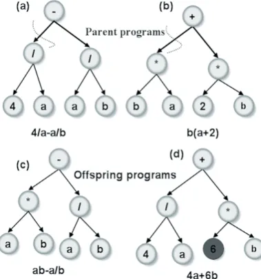
Figure 1.Symbolic representation of parent and offspring genetic programs

In figure 1, two parent programs to model a physical phenomenon are shown. After testing these programs for their modelling performance, they are operated by cross-over operator. That is, parts of the programs are crossed over at the dashed locations to generate the offspring programs. Also, mutation is illustrated by arbitrarily changing the parameter 2 to 6.

showed that WGEP models are effective in forecasting daily precipitation with better performance over WNF models. Selle [6] utilized genetic programming to systematically develop alternative model structures with different complexity levels for hydrological modelling with the objective of testing whether GP can be used to identify the dominant processes within the hydrological system. Models were developed for predicting the deep percolation responses under surface irrigated pastures to different soil types, water table depths and water ponding times during surface irrigation. The dominant process in the model prediction as determined from the models generated using genetic programming was found to be comparable to those determined using conceptual models. Thus it was concluded that Genetic programming can be used to evaluate the structure of hydrological models. A common aspect of GP based modelling that all these studies reported is the fact that the GP modelling resulted in fairly simpler models which could be easily interpreted for the physical significance of the input variables in making a prediction. Jyothiprakash and Magar (2012) [12] performed a comparative study of reservoir inflow models developed using ANN, ANFIS and linear GP for lumped and distributed data. The study reported superior performance of GP models over ANN and ANFIS models.

2. Simple and interpretable hydrological models using genetic

programming

prediction could be readily identified from the model structure. When carefully implemented models can throw light into and identify the key physical processes contributing to the phenomenon predicted and hence the development of the model. This is an important feature lacking from many of the data mining based prediction models resulting from which these modelling approaches are often earmarked as “black-box” models. “Black-box” nature of the prediction models often result in the limited use of such models for practical predictive applications.

2.1. Model complexity of GP and neural networks – Comparative study

The authors had conducted a study [7] to evaluate the complexity of predictive models developed using Genetic programming in comparison with models developed using neural networks. The models based on GP and neural network were developed as potential surrogate models to a complex numerical groundwater flow and transport model. The saltwater intrusion levels at monitoring locations resulting due to the excitation of the aquifer by pumping from a number of groundwater pumping wells were modelled by using GP and neural networks. The pumping rates at these groundwater well locations for three different stress periods were the inputs or independent variables for the model. The resulting salinity levels at the monitoring locations were the dependent variables or outputs.

The ANN used in the study was trained in the supervised training mode using a back propagation algorithm. The objective function considered for both the GP and ANN training was minimization of the total root mean square error (RMSE) of the prediction. The prediction error was calculated as the difference between the model (GP or ANN) predicted values and the actual from the numerical model generated data set.

The input-hidden-output layer architecture for the ANN model was optimized by trial and error. Both GP and ANN models had 33 input variables and 3 outputs. The number of hidden neurons in the ANN model was determined by adding 1 hidden neuron during each trial. A sigmoid transfer function and a learning rate of 0.1 were used. In developing the model the back propagation algorithm modifies the connection weights connecting the input-hidden and output neurons by an amount proportional to the prediction error in each iteration and repeats this procedure numerous times till the prediction errors are minimized to a pre-specified level. Thus for any given model architecture (model structure) the neural network model optimizes the connection weights to accomplish satisfactory model predictions. Where as the genetic programming modelling approach is different in that it evolves the optimal model architecture and their respective parameters in achieving satisfactory predictions.

The GP models developed used a population size of 500, mutation and cross over frequencies of respectively 95 and 50 percent. The number of generations were not specified a priory, instead the evolutionary process was stopped when the fitness function was less than a critical value. In order to achieve the simplest models, the mathematical operators where initially kept a minimum and then further operators were added into the functional set. In this manner, initially addition and subtraction were alone added in this set and later the operators multiplication, arithmetic and data transfer were added into the set.

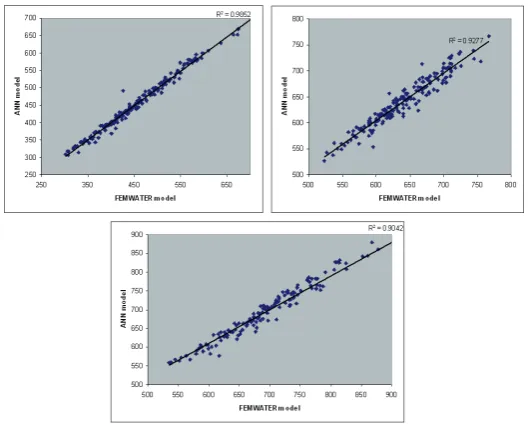
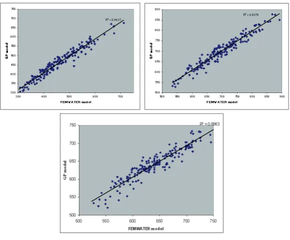
The predictive performance of the GP and ANN models on an independent set of data were found to be satisfactory in terms of the correlation coefficient and minimized RMSE. Figure 2 and 3 respectively shows the ANN and GP predictions of salinity levels at three monitoring locations corresponding to the their corresponding values from the numerical simulation model A dissection of the GP and ANN models were performed to evaluate the model complexity. The modelling framework of the GP models essentially has a functional set and a terminal set. The functional set comprises of the mathematical operations like addition, subtraction, division, multiplication, trigonometric functions etc. The terminal set of GP comprises of the model parameters which are also optimized simultaneously as the model structure is optimized. In our study the developed GP models used a maximum terminal set size of 30. i.e., satisfactory model predictions could be achieved with only 30 parameters for the GP model.

method. In the ANN approach where comparatively only a few models are tested in the trial and error approach which does not implement an organized search for better model architectures. The only components that are optimized during the development of the ANN model are the connection weights. Thus the model structure is rigid and is retained as determined by the trial and error procedure. This gives lesser flexibility in adapting the model structure with respect to the process being modelled. In our study it was found that while GP models required only 30 parameters in developing the model the number of connection weights in the ANN models was 1224. This is a metric of the simplicity of the GP models as against the ANN models. From figures 2 and 3 it is observed that despite the simplicity of the model and much lesser number of parameters used GP predictions are very similar to the ANN model predictions. For each hidden neuron added into the ANN architecture the number of connection weights increases by a number equal to the total number of inputs and outputs. Hence there is a geometric increase in the number of connection weights with increase in the number of hidden neurons in ANN architecture. The comparison of the number of parameters in itself testifies the ability of the genetic programming framework to develop simpler models. The impact of the number of parameters on the model is on the uncertainty of the predictions made using the model. The more the number of parameters, the more uncertainty in them and hence this uncertainty propagates into the predictions made.

3. Parsimonious selection of input variables

Another key feature of the genetic programming based modelling approach is the ability of genetic programming to identify the relative importance of the independent variables chosen as the modelling inputs. Many often in hydrological applications it is uncertain which variables are important to be included as inputs in modelling a physical phenomenon. Similarly time series models are used quite often in predicting or forecasting hydrological variables. For example the river stages measured on a few consecutive days can be used to forecast the river stage for the following days. In doing so the number of past days’ flow to be included as inputs into the time series model depends on the size and shape of the catchment and many similar parameters. Most often rigorous statistical tests like auto-correlation studies are conducted to determine whether an independent variable is significant to be included in the model development or not. Once included most often it is not possible to eliminate from most of the modelling frameworks because of the earlier mentioned rigidity of the model structure. For example, in neural networks an insignificant model input should be ideally assigned zero connection weights to the output. However, these connection weights most often don’t assume the zero value but converge to very small values near zero. This results in the insignificant variable being influencing the predictions made by a small amount. These results in uncertainties in the predictions made.

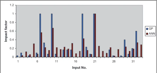
above to evaluate the parsimony in the selection of inputs for model development. GP evolves the best model structure and parameters by testing millions of alternate model structures. The relative importance of the each independent variable in the model development was computed by the recurrence of each independent variable in the best 30 models developed by GP. Thus, if an input appears in all the 30 models its impact factor is 1 and if one independent variable appears in none of the best 30 models its impact factor is 0.

Figure 2.Salinity predictions at three locations by the ANN models

To determine the significance of the inputs in the neural network model a connection weights method was used [7]. In this method the significance of each input is computed as a function of the connection weights which connects it to the output through the hidden layer. The formulae used in [7] were used to compute this;

1. First step in this approach was to compute the product of the input-hidden layer and hidden output layer weights. The, divide this by the sum of products of absolute values of the input-hidden and hidden output layer weights of all input neurons. This is given by Qih in (2)

, | , | | ,|

i h i h h o

P W  W ₍₁₎

1

ih

ih ni

ih i

P Q

P





2. Divide the sum of the Qih for each hidden neuron by the sum for each hidden neuron

of the sum for each input neuron ofQ_ih, for each i. The relative importance of all output weights attributable to the given input variable is then obtained. The relative importance is then mapped to a 0-1 scale with the most important variables assuming a value of 1. A RI value of 0 indicates an insignificant variable.

1

1 1

nh

ih h nh ni

ih h i

Q RI

Q



 







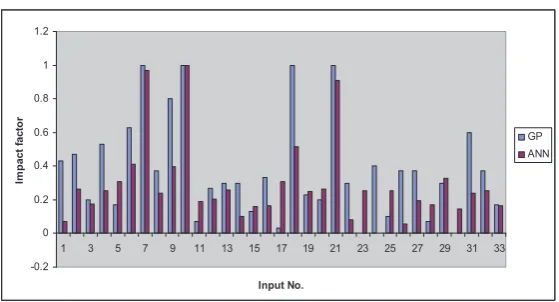
In this manner, the significance of each independent variable (input) to the model was quantified in a 0-1 range as impact factor and relative importance respectively for GP and ANN models. These values for GP and ANN models are plotted in figures 4,5 and 6.

Figure 4.Impact factors of input variables in predicting Salinity at location 1.

Figure 5.Impact factors of input variables in predicting Salinity at location 2.

From these figures it can be observed that all the variables considered has a non-zero impact in the developed ANN models. Whereas, GP is able to assign zero impact factor to those inputs which are not significant and thus able to eliminate them from the model. This helps in developing simpler models and reducing the predictive uncertainty. In figure 4 it can be seen that GP identified 13 inputs with zero impact factor. This implies that the pumping values corresponding to these inputs have negligible effect on the salinity levels at the observation location. Thus 13 out of the 33 inputs considered are eliminated from the GP models resulting in much simpler models compared to the ANN models where all the 33 inputs take part in predicting the salinity even though some of them are having very less impact on the predictions made. The ability of GP to eliminate insignificant variables is because of the evolutionary nature of model structure optimization. By performing cross-over, mutation and selection of candidate models over a number of generations GP is able to derive the optimum model structure with the most important input variables which are

0 0.2 0.4 0.6 0.8 1 1.2

1 6 11 16 21 26 31

Input No.

Im

pa

ct

fac

to

r

GP ANN

-0.2 0 0.2 0.4 0.6 0.8 1 1.2

1 3 5 7 9 11 13 15 17 19 21 23 25 27 29 31 33

Input No.

Im

pact

fac

to

r

relevant to the model prediction. This inturn help in developing simpler models with fewer uncertainties in the model prediction.

Figure 6.Impact factors of input variables in predicting Salinity at location 3.

4. Multiple predictive model structures using GP

The advent of GP as a modelling tool has paved the way for researches exploring the possibility of multiple optimal models for predicting hydrological processes. Genetic programming, in its evolutionary approach to derive optimal model structures and parameters, tests millions of model structures which can mimic the physical process under consideration. Researches have found that multiple models can be identified using GP which are considerably different in model structures but able to make consistently good predictions. Parasuraman and Elshorbagy [8] developed genetic programming based models for predicting the evapo-transporation. In doing so, multiple optimal GP models were trained and tested and they were applied to quantify the uncertainty in those models. Another study by the authors [9] developed ensemble surrogate models for predicting the aquifer responses to pumping in terms of salinity levels at observation locations. An ensemble of surrogate models based on GP was developed and the ensemble was used to get model predictions with improved reliability levels. The variance of the model predictions were used as the measure of uncertainty in the modelling process.

5. GP as surrogate model for simulation-optimization

A very important application of data intensive modelling approaches is to develop surrogate models to computationally complex numerical simulation models. As detailed elsewhere in this article, the authors have utilized GP in developing potential surrogates to a complex density dependent groundwater flow and transport simulation model. The potential utility of the surrogates is to replace the numerical simulation model in simulation-optimization frameworks. Simulation-simulation-optimization models are used to derive optimal management decisions using optimization algorithms in which a numerical simulation

0 0.2 0.4 0.6 0.8 1 1.2

1 6 11 16 21 26 31 Input No.

Im

pa

ct

fa

ct

or

models is run to predict the outcome of implementing the alternative management options. For example, the authors developed simulation-optimization models to develop optimal management decisions for coastal aquifers. The optimal pumping from the coastal aquifer can be decided only by considering the impact of any alternative pumping strategy on saltwater intrusion. For this the numerical simulation model needs to be integrated with the optimization algorithm and the impact of each candidate pumping strategy is predicted by using the simulation model iteratively. This involve a lot of computational burden as thousands of numerical model runs are required before an optimal pumping strategy is identified.

GP was used a surrogate model within the optimization algorithm as a substitute of the numerical simulation model in our study (Sreekanth and Datta, 2010). Previous studies have used artificial neural networks as surrogate models to replace groundwater numerical simulation models. Emily et a1 (2005) used genetic programming based surrogate models for groundwater pollution source identification. In our study (Sreekanth and Datta, 2010), it was found that genetic programming could be used as a superior surrogate model in such application with definite advantages. The study intended to develop optimal pumping strategies for coastal aquifers in which the total pumping could be maximized and at the same time limiting the saltwater intrusion at pre-specified limits. In doing so, the effect of pumping on the salinity levels was predicted using trained and tested GP models. The GP models were externally coupled to a genetic algorithm based optimization model to derive the optimal management strategies. The results of the GP based simulation-optimization was then compared to the results obtained using an ANN-based simulation-optimization model. The ability of GP in parsimoniously identifying the model inputs helped in reducing the dimension of the decision space in which modelling and optimization was carried out. The smaller dimension of the modelling space helped in reducing the training and testing required to develop the surrogate models. The study identified that GP has potential applicability in developing surrogate models with potential application in simulation-optimization methodology to solve environmental management problems.

6. Conclusion

1. Genetic programming is able to develop simple models for developing the time series forecast models. When compared to the complex architecture of neural networks the GP models are simpler and easy to analyse. This is particularly relevant in developing transparent models for predicting natural phenomena. Complex neural network architectures make ANN model more or less “black-box” in nature, where as simpler GP models makes it easy to analyse the physical significance of each input in the model development.

2. In GP modeling, the optimum model architecture is evolved by GP after testing, most often, millions of alternate model structures and parameters as against the trial and error approach being followed by other artificial intelligence modeling approaches like neural networks. This helps in converging to global optimal solutions in minimizing the error criteria used for model development. Thus GP is able to develop global optimum models for predicting/forecasting hydrological processes and time series.

3. Genetic programming has the capability of parsimoniously selecting the variables for model development from the potential inputs. This helps to prevent redundancy in model development in terms of unnecessary inputs and parameters. In course of the model development GP determines the significance of each input in the model development in an efficient way so that the totally insignificant inputs are eliminated from the model. As shown in the results approaches like neural network models are also able to identify the relative significance of the inputs, they are less efficient in achieving this because of the rigidity of the model structure and connection weights. These key advantages of GP modeling are illustrated using realistic example in the broad area of hydrology and groundwater management for time series model development and conclusions are drawn which establishes the potential of genetic programming as a modeling and prediction tool for hydrology and water resources application.

Author details

J. Sreekanth1,2,3 _{and Bithin Datta}1,2

1_{CSIRO Land and Water, Ecosciences Precinct, Australia}

2_{Discipline of Civil and Environmental Engineering,}

School of Engineering and Physical Sciences, James Cook University, Townsville, Australia

3_{CRC for Contaminant Assessment and Remediation of the Environment, Mawson Lakes, Australia}

7. References

[1] Koza, J.R., 1994. Genetic programming as a means for programming computers by natural selection. Statistics and Computing, 4(2): 87-112.

[3] Rabunal, J. R., Puertas, J., Suarez, J., and Rivero, D. (2006) Determination of the unit hydrograph of a typical urban basin using genetic programming and artificial neural networks Hydrological Processes, vol. 21, Issue 4, pp.476-485

[4] Rahman Khatibi, Mohammad Ali Ghorbani, Mahsa Hasanpour Kashani and Ozgur Kisi (2011) Coparison of three artificial intelligence techniques for discharge routing, Jorunal of Hydrology, 403(3-4), 201-212.

[5] Ozgur Kisi and Jalal Shiri (2010), Precipitation forecasting using wavelet genetic programming and wavelet neuro fuzzy conjunction models, Water Resources Management, 25(13), 3135-3152.

[6] Benne Selle, Nithin Muttil (2010), Testing the structure of a hydrological model using genetic programming, Journal of Hydrology, 397(1-2), 1-9.

[7] Sreekanth, J., and Bithin, Datta., (2011), Comparative evaluation of Genetic Programming and Neural Networks as potential surrogate models for coastal aquifer management, Journal of Water Resources Management, 25, 3201 – 3218. (doi: 10.1007/s11269-011-9852-8)

[8] Parasuraman, K., Elshorbagy, A., 2008. Toward improving the reliability of hydrologic prediction: Model structure uncertainty and its quantification using ensemble-based genetic programming framework. Water Resources Research, 44(12).

[9] Sreekanth, J., and Bithin, Datta., (2011), Coupled simulation-optimization model for coastal aquifer management using genetic programming based ensemble surrogate models and multiple realization optimization, Water Resources Research, 47, W04516, doi: 10.1029/2010WR009683

[10]Sreekanth, J., and Bithin, Datta., (2010), Multi-objective management of saltwater intrusion in coastal aquifers using genetic programming and modular neural network based surrogate models, Journal of Hydrology, 393 (3-4), 245-256

[11]Emily, Zechman, Baha, Mirghani, G, Mahinthakumar and S Ranji Ranjithan (2005) A genetic programming based surrogate model development and its application to a groundwater source identification problem, ASCE conf. Proc. 173, 341.