City, University of London Institutional Repository
Citation: Cowell, R. (2013). A simple greedy algorithm for reconstructing pedigrees.
Theoretical Population Biology, 83, pp. 55-63. doi: 10.1016/j.tpb.2012.11.002
This is the accepted version of the paper.
This version of the publication may differ from the final published
version.
Permanent repository link: http://openaccess.city.ac.uk/6011/
Link to published version: http://dx.doi.org/10.1016/j.tpb.2012.11.002
Copyright and reuse: City Research Online aims to make research
outputs of City, University of London available to a wider audience.
Copyright and Moral Rights remain with the author(s) and/or copyright
holders. URLs from City Research Online may be freely distributed and
linked to.
City Research Online: http://openaccess.city.ac.uk/ [email protected]
A simple greedy algorithm for reconstructing pedigrees
Robert G. Cowell∗,a
aFaculty of Actuarial Science and Insurance, Cass Business School, 106 Bunhill Row,
London EC1Y 8TZ, UK
Abstract
This paper introduces a simple greedy-search algorithm for finding high-likelihood pedigrees using micro-satellite (STR) genotype information on a complete sam-ple of related individuals. The core idea behind the algorithm is not new, but it is believed that putting it into a greedy search setting, and specifically the application to pedigree learning, is novel. The algorithm does not exploit age or sex information, but this information can be incorporated if desired. Prior infor-mation concerning pedigree structure is readily incorporatedafter the greedy-search is completed, on the high-likelihood pedigrees found. The algorithm is applied to human and non-human genetic data and in a simulation study.
Key words:
Pedigree reconstruction, maximum likelihood pedigree, greedy search.
1. Introduction
The reconstruction or estimation of pedigrees of individuals finds applica-tions in both human and non-human populaapplica-tions, for reviews see (Jones and Ardren, 2003; Blouin, 2003; Pemberton, 2008). This paper considers the statis-tical estimation of pedigrees using genotype markers for a complete sample of individuals. Maximum likelihood pedigree estimation was developed by Thomp-son (1976, 1986) using age and sex information. Almudevar (2003) proposed a simulated annealing approach that avoids the need for age and sex information. Cowell (2009) adapted the Bayesian network learning algorithm of Silander and Myllym¨akki (2006) to develop an exhaustive search algorithm that is guaranteed to find a pedigree of highest likelihood; the algorithm has complexityO(n32n)
in the numbernof individuals, but is computationally feasible for up to around 30 individuals. A constraint-based integer programming approach is presented in (Cussens, 2010; Cussens et al., 2012) that can find maximum likelihood pedi-grees involving more than 30 individuals, giving examples of pedipedi-grees of up to 64 individuals. Using the same algorithm the second, third,. . . , kth highest likelihood pedigrees may be found by imposing additional constraints as each
high-likelihood pedigree is found (Cussens et al., 2012). It is also possible to extend the algorithm of Cowell (2009), along the lines that Tian et al. (2010) use for general Bayesian networks, to find the k highest likelihood pedigrees; however the complexity grows asO(kn32n), thus limitingkto a relatively small number.
The algorithm presented in this paper grew out of the desire to find a large set of high likelihood pedigrcussens:etal:2012ees, rather than a single maximum likelihood pedigree. It uses a simple procedure of selecting one pedigree at a time, and deriving from the selected pedigree a set of candidate pedigrees by a partitioning process described below. A feature of the partitioning process is that the candidate pedigrees could have a very different structure to the pedigree that they are generated from. In addition, the partitioning process in principle covers the space of all possible pedigrees on the set of individuals, without duplicating any pedigree.
The next section introduces the partitioning algorithm in the context of finding the bestk-spanning trees of an undirected graph. (This is closely related to finding pedigrees in which each individual has at most one parent in the pedigree.) The pedigree search algorithm using the partitioning is presented in Section 3. The algorithm is then applied to human and animal data, and in a simulation study, in Section 4.
2. Finding the k best spanning trees of a graph
Before presenting the pedigree search algorithm, we first present a variation of the algorithm that can find thek highest weight spanning trees of an undi-rected graph. The algorithm is given by S¨orensen and Janssens (2005) (who looked for lowest weight spanning trees, rather than highest weight spanning trees). Suppose that we are given an undirected connected graph onnvertices, in which each edge between a pair of vertices is given a non-negative weight value. A spanning tree is a connected subgraph containing all n vertices and
n−1 edges, but does not have a cycle. The weight of the spanning tree is the sum of the weights of the edges of the spanning tree. The problem is to find a set of k spanning trees such that no other spanning tree has a weight greater than any spanning tree in the set of thekspanning trees.
A well known algorithm for finding the highest scoring spanning tree is Kruskal’s algorithm (Kruskal, 1956), which we describe as follows. Let the nodes of a graphGbe labelled by the integers from 1 ton. We form an ordered list L of the E edges, which are sorted in order of decreasing weight, with the first entry denoted by L(1), the second by L(2), ... , up to L(E). The algorithm starts with an initial graphF having no edges between thennodes. The algorithm is simply to work through the weight-ordered edges inL, adding an edge toF if in doing so it does not create a cycle, untilF is fully connected. It is illustrated in Algorithm 1.
Note that the first edge in the list is always added (because it cannot form a cycle by itself). Suppose that the maximum weight spanning tree
input : An undirected edge-weighted graphGinnvertices; a listLof theE edges ofGsorted in decreasing weight; a totally disconnected graphF on thenvertices.
output:F as the maximum weight spanning tree ofG.
1, . . . , nInitialization: Seti←1.
while F is not connected do
Add edgeL(i) to F if it does not create a cycle.
i←i+ 1
end
Algorithm 1: Kruskal’s algorithm for finding the maximum weight spanning
tree of an undirected graph
e1
1(= 1), e12, e13, . . . , e1n−1 of the entries in the list L. If S denotes the space
of spanning trees of G, then the second highest-weight spanning tree F2 of S
is the highest inS− F1. (Note it is possible that F1 andF2 might have the
same weight.) Let us denote the listLedge indices ofF2bye2
1, e22, e23, . . . , e2n−1.
Now becauseF1andF2are distinct trees, they must differ in at least one edge.
Therefore (exactly) one of the followingn−1 conditions must be true:
e21> e11 (1a)
e21=e11&e22> e12 (1b)
e21=e11&e22=e12&e23> e13 (1c) ..
.
e21=e11&e22=e12&. . . & en2−2=e1n−2&e2n−1> e1n−1 (1d)
Hence, the procedure for finding the second highest weight spanning tree is to carry out Kruskal’s algorithm n−1 times, the first time excluding e1
1 from
the list L(constraint 1a), the second time including e1
1 but excludinge12 (1b),
and so on. From the set of n−1 trees found, pick the one having the highest weight (breaking ties arbitrarily if necessary), thus givingF2. Now suppose that
we want the third highest weight spanning treeF3. Then it is either amongst
the remaining n−2 candidate trees found during the search forF2, or it has
edges with indicese3
1, e32, e33, . . . , e3n−1where one of the following holds to ensure
it differs fromF2in at least one edge:
e31> e21 (2a)
e31=e21&e32> e22 (2b)
e31=e21&e32=e22&e33> e23 (2c) ..
.
By applying Kruskal’s algorithm again several times, using these constraints,
F3 may be identified. Note the first constraint (2a) is equivalent to removing
the firste21 edges from the listL, whilst for the other possible trees the search
is started at the e21 edge (2b - 2d). The procedure may be repeated until the
desired number k of maximum weight spanning trees is found, see S¨orensen and Janssens (2005) for more details and proof. Note that if the procedure is repeated with no upper boundkspecified, then the algorithm will generate all possible spanning trees ordered by weight. It does not carry forever because for some trees the final edge added will be the last in the listL, and so for these the tree-search cannot be split on the last edge (2d). One can fruitfully view the partitioning as generating a binary search over the space of spanning trees, similar to but distinct from the standard depth-first search algorithm.
S¨orensen and Janssens (2005) based their algorithm on one by Murty (1968) for finding thekbest assignments; the latter was generalised by Lawler (1972). This idea of partitioning the search space into exclusive and exhaustive parts was also used in a probabilistic setting by Nilsson (1998) in an application to find the k highest probability configurations of discrete random variables having a joint distribution defined over a junction tree. Note that the k-th stage of the maximum-weight spanning tree algorithm gives the k-th highest weight tree. This is a consequence of the fact that Kruskal’s greedy search algorithm is optimal for returning the highest weight spanning tree. The best
kcombinatorial search applications cited above combine the partitioning with anoptimal procedure (such as Kruskal’s algorithm) to find the kbest-optimal configurations (of whatever combinatorial structure is being searched for). The simple idea in this paper is to use the exclusive and exhaustive partitioning procedure combined with a greedy rather than an optimal procedure to guide the search, in this paper over the space of high-likelihood pedigrees. This simple adaptation of an old algorithm appears to be novel, but quite powerful.
3. Pedigree search algorithm
3.1. Finding the local scores
We will consider the special case of learning pedigrees with complete data. This means that a parent of an individual is either in the sample, or if not the parent is unrelated to all other members in the sample. Under this assumption, the likelihood function for a given pedigree decomposes into a simple multi-plicative form. A pedigree onn individuals (numbered from 1 up to n) may be represented by a directed-acyclic graphG on nnodes, in which each node represents the genotype of an individual. An arrow from node j to node i in-dicates that j is a parent of i. The graph has no directed cycles, to avoid an individual being their own ancestor. Each node ofGhas one of three possible parent configurations:
struct Score {
integer child, parent1, parent2; real value;
}
Figure 1: Scoredata structure used for storing invaluethe log-likelihood of an individual’s genotype given the genotypes of the specified parents. Note that bothparent1andparent2
being zero, corresponds to the score ifchildis a founder.
• The node has one incoming arrow. Hence the individual has only one parent specified in the pedigree.
• The node has two incoming arrows. Hence both parents of the individual are in the pedigree.
Let gi represent the genotype of the i-th individual. Then we let p(gi|gj, gk)
denote the conditional probability that individualiwill have genotypegi given
that it has the two parentsj andkin the pedigreeGhaving genotypesgj and
gk respectively. Ifi has only one specified parent, sayj then it has conditional
probabilityp(gi|gj), and if no parents then probabilityp(gi). If we letgπidenote
the genotypes of the parentsπi ofi in the sample, then the log-likelihood of a
pedigree having parent-sets{πi|i= 1, . . . , n}decomposes into the additive form:
l(G) =
n
X
i=1
logp(gi|gπi). (3)
The pedigree search algorithm requires the evaluation of every possible
p(gi|gπi) term, but this is carried out only once. If the markers are independent,
then eachp(gi|πi) term is itself a product of terms one for each markerm:
p(gi|gπi) =
Y
m
p(gim|gπm
i).
This decomposable form of the overall log-likelihood into local score con-tributions is used in the pedigree search algorithm. Like the spanning tree algorithm, a sorted list is formed. In this case the elements of the list are the local scores logp(gi|gπi) together with the child node i and the parent-set πi
ofi. We store them in the following Score data structure, shown in Figure 1. If S is a instance of a score, then S.childgives the index ∈ {1, . . . , n} of the child individual, and so on. The algorithm for making the list of local scores is outlined in Algorithm 2.
We now introduce a structure Pedigree. This is a directed graph with n
input : A set ofnindividuals and their genotypes {gi:i= 1, . . . , n}
output: A sorted listLof|L| local scores.
initialization: SetL← ∅.;
foreach i∈1, . . . , n do
foreach possible parent-set π ofi having genotypegπi do if p(gi|gπi)>0 then
Add a ScoreinstanceSto the listLwhere:
S.child=i;
S.parent1andS.parent2store the indices of the
possible parentsπi, (either or both may take the value zero);
S.value= logp(gi|gπi).
end end end
Sort the listLof scoresbyn decreasing order of their values.
Algorithm 2: Making the local scores list
pedigree in which every is a founder. Instead in the pedigree we store for each individual a boolean variable to indicate whether the individual’s parent-set has been specified. It is initially set toFalse for every individual, and it is set to
True when an individual’s parent-set has been specified — this could include the case that the individual is specified to be a founder.
A pedigree is built up by adding parent-sets to each individual, with one parent-set per individual, and a pedigree is fully specified when all parent-sets have been specified. However the process of attempting to add a parent-set of an individual might make an invalid pedigree in by introducing a directed cy-cle in the pedigree graph. We introduce a function AddParents(Pedigree P,
Score S)that takes as inputs a current partially specified Pedigree P and a
Score S. If the Scorestructure S has a child valueS.child that has already
hadS.child’s parent-set specified in Pthen the function returnsFalse.
Oth-erwise if the parent-set specified by S.parent1 and S.parent2, can be made parents of S.child without creating a cycle, then the function modifies Pby adding these individuals as parents of S.child (by adding a directed edge
S.parent1→S.childifS.parent1>0, and a directed edgeS.parent2→S.child
if S.parent2>0) and returns True; if however adding them as parents would
create a directed cycle then the function returnsFalse without modifyingP.
3.2. Making a single pedigree from the local scores
configuration from the local-scores list that is as high as possible. However the pedigree it makes will not necessarily achieve the maximum possible likelihood (unlike the situation for Kruskal’s algorithm). Each time a parent-set is specified in the pedigree as it is being built up, it increments a counter C that counts the number of parent-sets that have been specified. It stops whenC=n, which occurs when every individual has had their parent-set specified. Note that the list L will always contains the scores for every individual in which they are founders (corresponding to πi =∅ for each i), thus a valid pedigree is always
returned. Note also that the log-likelihood associated with the pedigree is the sum of the values of the scores for which adding parent-sets was successful. We assume that this total log-likelihood is stored in the pedigree in the quantity
value.
input : The sorted listL of local scores.
output: A valid pedigree over thenindividuals.
initialization:
APedigree Pofnindividuals with specified no parent-sets.
P.value←0
An integerC←0
for i from 1 to|L| do
if AddParent(P, L(i)) is true then
C←C+ 1;
P.value←P.value+L(i).value;
end
if C=nthen
STOPand returnP.
end end
Algorithm 3: MakePedigree(L): Making a pedigree from a listLof ordered
local scores.
3.3. The pedigree greedy search algorithm
We now combine the pedigree construction algorithm of Algorithm 3 with the partitioning algorithm, to carry out a greedy search over the space of possible pedigrees, giving two variants of the algorithm, which we shall callVariant 1
and Variant 2. Note that in forming a pedigree using Algorithm 3, n scores
We make the first pedigreeP1with Algorithm 3. SupposeP1has been made with the scores having the indices in the listL given bye11(= 1), e12, e13, . . . , e1n, which are stored in the arrayindex inP1 denoted byP1.index. Hence for this pedigreeP1.index[i] =e1i, and we setP1.fixed= 1. The next stage is to make the set of candidate pedigrees, one from each of the following constraints:
e21> e11 (4a)
e21=e11&e22> e12 (4b)
e21=e11&e22=e12&e23> e13 (4c) ..
.
e21=e11&e22=e12&. . . & e2n−1=e1n−1&e2n> e1n (4d)
A pedigree made with the first constraint (4a) may be made by applying Algorithm 3 using the listL, but starting theiiteration frome11+ 1 instead of
e11. A pedigree made from the second constraint (4b) may be made by adding the parent-set associated with scoreL(e11), and completed by running for iterative
loop of Algorithm 3 fromi = e12+ 1. In general the pedigree made from the j-th constraint is made by creating a pedigree that adds the parent-sets of the scores L(e1
1), L(e12), . . . , L(e1j−1) used in makingP1, and continuing the i loop
fromi=e1
j+ 1. For the pedigree made with thej-th constraint we store in its
fixedvalue the integerj.
In Variant 1 of the algorithm, each of these pedigrees is inserted into a
priority queue Queue that automatically keeps the pedigrees in their order of decreasing (or more accurately, non-increasing) log-likelihood. When all candi-date pedigrees have been made, the pedigree at the front of the queue will be pedigreeP2, and may be removed.
The pedigree P3 is made by making a new set of pedigrees from P2 and inserting them intoQueue. P3 will then be at the front of Queue. To generate the set of pedigrees from P2 we apply one of the following constraints, which uses thefixedvalue stored inP2 when it was formed. Letf =P2.fixed. Then the constraints are:
e31=e21&e32=e22&. . . & e2f−1=e2f−1&e2f >e2f
e31=e21&e32=e22&. . . & e3f =e2f &e3f+1>e2f+1
.. .
e31=e21&e32=e22&. . . & e3n−1=e2n−1&e3n>e2n
(5)
The reason for not looking at pedigrees with constraints such as, for example,
is that this constraint is equivalent to
e31=e11&e32=e12&. . . & ef3−2=e1f−2&e2f−1> e1f−1
which was the constraint applied to find P2 from P1. Similarly, the other con-straints corresponding to some candidate pedigree generated from P1 and al-ready in Queue. This is the reason for introducing the fixed value for each pedigree, it prevents a pedigree from being generated more than once.
We are now ready to give the greedy pedigree search algorithm, which is laid out in Algorithm 4. The pedigree found at stage k is be stored in a list
PedList, which is a first-in-first-out list. Intermediate pedigrees are stored in
Queuewhich initially is empty. We suppose that we wish to continue the search
until there are K pedigrees inPedList. (Note that these will not necessarily be theK highest likelihood pedigrees.) Note that if the condition (k < K−1) is removed, then the algorithm will generate all possible pedigrees that can be formed out of selection of thenparent-sets from the set of local scores, that is, it does an exhaustive generation of possible (positive likelihood) pedigrees.
InVariant 2of the algorithm, we simply make Queueto be a
first-in-first-out queue instead of a priority queue. As we shall see this can perform well.
Variant 3will be introduced in Section 4.
3.4. Special case: Single parent pedigrees
Suppose that in forming the list L of local scores, we do not include any scores in which an individual has two parents, so the local scores are only for individuals that are founders or have one parent amongst the n individuals. Then Algorithm 3 is equivalent to Kruskal’s search algorithm andVariant 1of Algorithm 4 is essentially that of S¨orensen and Janssens (2005), but instead of generating undirected maximum spanning weight trees in the order of decreasing weight, it generates pedigrees in order of decreasing likelihood, in which no individual has more than one parent. One minor difference it that topologically, each such pedigree need not be connected, so graphically the pedigree could be a forest of directed trees rather than a single connected tree. This arises because the local scores contain terms in which individuals are founders; in contrast in the spanning tree algorithm the weights are only ever between edges of pairs of nodes.
3.5. Bounding the greedy search algorithm
As mentioned in Section 3.3, removing the condition k < K−1 from the
while loop of Algorithm4 means that all possible (positive likelihood)
input : The sorted listL of local scores;
A queueQueueof candidate pedigrees, initially empty;
PedListof found pedigrees, initially empty.
initialization:
Pedigree P= MakePedigree(L);
P.fixed= 1;
InsertPintoQueue;
k←0.
search iterations:
whileQueue is not empty and k < K−1do
k←k+ 1;
Remove the first pedigree fromQueue, call it Pk; InsertPk toPedList.
for ifrom Pk.fixeduntil ndo
Make new initializedPedigree P;
C←0;
for j from 1 toPk.fixed−1do
AddParent(P, L(Pk.index[j]));
C←C+ 1;
end
P.fixed←i;
forj fromPk.fixed+ 1 until|L|do if AddParent(P, L(j))is true then
C←C+ 1;
P.value←P.value+L(i).value;
end end
if C=nthen
InsertPintoQueue else
DiscardP end
end end
k←k+ 1;
Remove the first pedigree fromQueue, call itPk;
InsertPk intoPedList.
Algorithm 4: Greedy pedigree search to find K high-likelihood pedigrees.
InVariant 1of the algorithm, Queueis a priority queue, with highest
However it is possible to introduce a bounding condition so that for not too many individuals the algorithm terminates in reasonable time and the maxi-mum likelihood pedigree is thus identified. The modification of Algorithm 4 to achieve this is straightforward, and is as follows.
Consider the state of the pedigreePformed fromPkafter the first of the inner
j-loops. This will be in a state in which the parent-sets ofC individuals have been specified, which means that there are a furthern−Cindividuals’ parent-sets to specify. We also have the log-likelihood of the pedigree contributed by theC individuals stored inP.value. So if we now add up the highest score of each of the n−C individuals in the list from the scores located from position
1+Pk.index[Pk.fixed]up to|L|, and add this total toP.value, we will get an
upper bound of the log-likelihood of any possible pedigree completion of P. If this is lower than the log-likelihood of the current best pedigree (which value is kept track of during the execution of the algorithm) then we may discardP, and not add it or any completion toQueue. Hence some potentially large sections of the pedigree search space can be disregarded as they are irrelevant to finding the highest likelihood pedigree.
4. Computer evaluations
Here is a summary of computer evaluations of the performance of the al-gorithm. All computations were carried out using a computer with an AMD dual-core 1.96GHz processor and 7GB of ram running the Debian 6 (squeeze) Linux operating system. In all evaluations Hardy-Weinberg equilibrium was assumed.
4.1. Romanov data
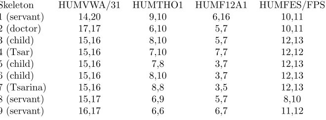
In July 1991, in a shallow grave 20 miles from Ekaterinburg, Russia, nine skeletons were found, some of which were believed to be the the remains of Tsar Nicholas II, his wife, three of their five children. This was confirmed in careful DNA analysis by (Gill et al., 1994). Table 4.1 shows STR genotype data for the nine skeletons and their designated identification as given in (Gill et al., 1994).
Skeleton HUMVWA/31 HUMTHO1 HUMF12A1 HUMFES/FPS
1 (servant) 14,20 9,10 6,16 10,11
2 (doctor) 17,17 6,10 5,7 10,11
3 (child) 15,16 8,10 5,7 12,13
4 (Tsar) 15,16 7,10 7,7 12,12
5 (child) 15,16 7,8 3,7 12,13
6 (child) 15,16 8,10 3,7 12,13
7 (Tsarina) 15,16 8,8 3,5 12,13
8 (servant) 15,17 6,9 5,7 8,10
[image:12.612.142.472.526.648.2]9 (servant) 16,17 6,6 6,7 11,12
Variant 1of Algorithm 4 was run with no upper boundK of the number of iterations of thewhile loop, and without the bounding procedure described in Section 3.5, so that all possible pedigrees were generated. (In the absence of suitable population allele frequencies, each marker was assumed to consist of eight alleles, (inclusive of the ones in the table), with a uniform distribution.) As mentioned above there are 11512 possible pedigrees (using sex information). The top-left plot in Figure 2 shows the log-likelihoods of the pedigrees in the order that they were added to thePedList, (that is P1,P2,. . . , P11512). The
highest likelihood pedigree wasP2. We see from the plot that there is generally
a steady decrease in the log-likelihood but with occasional increases, and that many of the pedigrees have log-likelihoods much lower than the highest value. The likelihood of the most likely pedigree is 1.81×10−39, which amounts to
approximately 10% of the sum of the likelihoods at 1.71×10−38. The first 254
pedigrees account for 95% of the total likelihood of all the pedigrees, the first 266 for 99% of the total. The top-left plot of Figure 2 shows the cumulative sum of likelihoods of the first k pedigrees found as a ratio to the sum of the likelihoods of all 11512 pedigrees, plotted fork values up to 300. Equivalent plots for Variant 2 are shown on the bottom panel of Figure 2 for which: the first 254 pedigree account of 78.3% of the total likelihood, the 95% level is reached on pedigree 513, and the 99% level at pedigree 863. We see that for this dataset Variant 1is being more efficient at picking out the higher likelihood pedigrees.
4.2. Simulation with a known pedigree of 20 individuals
A simulation study was carried out using the highly inbred pedigree of twenty individuals taken from (Cowell, 2009), shown in Figure 3. In each of one thou-sand simulations, genotypes were simulated for all the individuals consistent with parentage assignments in the pedigree, the maximum likelihood pedigree was found using the algorithm described in (Cowell, 2009), using sex informa-tion, and the log-likelihood was recorded. Algorithm 4 was also run, either until it found a pedigree having the maximum likelihood, or K = 5 million pedi-grees were put in thePedList. The bounding described in Section 3.5 was not employed in the search. The iteration of the highest likelihood pedigree found by the greedy search algorithm was recorded, together with the log-likelihood achieved. The log-likelihood of the generating pedigree was also recorded. The results fromVariant 1 and Variant 2for the same generated genotypes are markedly different.
Variant 1
0 2000 4000 6000 8000 10000 12000
−130
−120
−110
−100
−90
Variant 1
k
Log Lik
elihood
0 50 100 150 200 250 300
0.0
0.2
0.4
0.6
0.8
1.0
Variant 1
k
Cum. rel. lik
elihood
0 2000 4000 6000 8000 10000 12000
−130
−120
−110
−100
−90
Variant 2
k
Log Lik
elihood
0 50 100 150 200 250 300
0.0
0.2
0.4
0.6
0.8
1.0
Variant 2
k
Cum. rel. lik
[image:14.612.125.477.151.392.2]elihood
Figure 2: Log-likelihoods of pedigrees found from the Romanov data of nine individuals, in the order found. Top left: all 11512 pedigrees usingVariant 1, top right, the normalized cumulative likelihoods to the first 300 pedigrees, usingVariant 1. Bottom row: as for top row but withVariant 2of Algorithm 4.
[image:14.612.224.388.488.633.2]0e+00 2e+04 4e+04 6e+04 8e+04 1e+05
−310
−300
−290
−280
−270
k
Log lik
[image:15.612.140.462.143.352.2]elihood
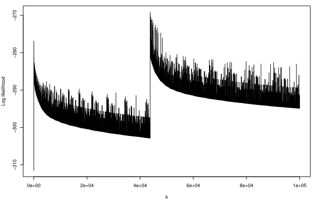
Figure 4: The log-likelihoods of the first 100,000 pedigrees, where the maximum occurred at iteration 43769.
log-likelihoods of the first 100,000 pedigrees found by the search algorithm for a run in which the maximum was found on iteration 43769. Note that until the jump to this pedigree, the plot gives the impression that the highest likelihood pedigree has been found on the second iteration. Although such trace plots can be suggestive that a maximum likelihood has been found, they can be misleading as this example shows. From the runs that did find the highest likelihood pedigree, the greatest number of iterations taken to do so was 3473461.
Note that in all of these runs the bounding strategy described in Section 3.5 was not used, so that the greedy algorithm did not identify the true maximum. The example from Figure 4 was re-run using the bounding technique. The computation took used 28587 iterations altogether for a complete search of pedigree space, with the highest likelihood pedigree found on iteration 9198.
Algorithm 4 with the bounding strategy was also re-run on each of the 16 pedigrees for which the algorithm without bounding failed to find the maximum pedigree after 5 million iterations. A limit was again set to 5 million iterations. In 14 out of the 16 runs, the highest likelihood pedigree was found, with three requiring over 1 million iterations.
Variant 2
The same sets of genotypes for the 1000 simulations for Variant 1 were used forVariant 2analyses, initially without using the bounding. For 255 of the runs, the first pedigree was the highest likelihood pedigree, (the same as
greedily selected pedigree). For 285 runs it was the second. For the remainder of the runs, there is a gap until the 9-th iteration to finding the highest likelihood pedigree. In 908 runs the highest pedigree was found within 1000 iterations, rising to 972 runs for up to 10000 iterations, and 994 for 100000 iterations. Of the remaining six pedigrees, five took from 104222 to 342247 iterations to find the highest pedigree, the remaining one took 7830717 iterations. In contrast, usingVariant 1the latter was found in in 541093 iterations.
However whenVariant 2of the algorithm was used with bounding,all runs found the highest likelihood pedigree, the longest run taking 32427 iterations, the next longest 14321 iterations.
Variant 3
In many pedigree search algorithms, such as those based on backtracking or MCMC search, the search procedure moves around pedigree space making small local changes to pedigrees, such as adding a parent, removing a parent, or reversing the rˆole of parent and child relationship, so that successive pedigrees are very close in structure, differing in one or two edges. Such algorithms can spend a lot of time searching a poor part of pedigree space, or even getting trapped at a local maximum. The motivation behind Algorithm 4 is that the pedigrees produced by the partitioning would be well spread out in pedigree space, so that two such pedigrees can differ dramatically in structure. This it is hoped would make the search range widely over pedigree space. ForVariant 1the focus is always on the currently best partition found. This appears to do well as show in the Figure 2. However, Figure 4 shows thatVariant 1is not immune from the problems of getting stuck for a long time in the vicinity of a local maximum. Variant 2 of Algorithm 4 is akin to a breadth-first search amongst the partitions, so that the successive pedigrees being found are located far apart in pedigree space in terms of their structural differences. This appears to be better thanVariant 1, in that it is more successful in finding the highest pedigree, though the number of iterations required has a long tail, with six pedi-grees requiring more than 100,000 iterations, without bounding, but drastically reduced with bounding. However it does not have the greedy focus ofVariant 1in choosing the order in which pedigrees are examined.
The motivation behind Variant 3 is to combine aspects of both of these searches into one that is more greedy thanVariant 2but less thanVariant 1. The idea is simple: Algorithm 4 is run asVariant 2using the first-in-first-out
Queue, but periodically after a fixed number of iterations has been performed,
Queueis sorted so that the highest likelihood pedigrees are at the front of the
list.
The five pedigrees that took more than 10000 iterations to find the high-est pedigree using the Variant 2with bounding were selected and this extra periodic sorting step was applied, both with and without bounding. Sorting was carried out every 10000 iterations (which meant that for the first 10000 iterations the algorithm behaves the same asVariant 2). The number of iter-ations in each case are laid out in Table 4.2, which also includes analyses using
would seem thatVariant 3performs best, however the application of bounding has a mixed response. In addition, the performance does depend upon the pe-riod used between sorts, as illustrated in the last row in the table. Note that for
theVariant 3runs, the pedigree is marked as found when it is removed from
Queuerather than when it is put intoQueue, which is the reason why several of
the values in the table are 1 above a multiple of 1000 or 10000.
Algorithm Pedigree
1 2 3 4 5
[image:17.612.136.472.208.317.2]Variant 1 no bound NF 1441427 NF 541093 129209 Variant 1 with bound 665086 225180 73866 12639 28726 Variant 2 no bounding 246622 95589 198140 NF 106065 Variant 2 with bounding 32427 14321 13525 10684 13413 Variant 3 no bounding 30001 20001 30002 60003 20001 Variant 3 with bounding 20001 10001 10002 10003 10001 Variant 3 with bounding∗ 4001 3001 4002 15003 3001
Table 2: Comparison of of iterations required by some some selected pedigrees to find highest pedigree, NF denotes not found within 5 million iterations. ∗Bottom row: period between sorts 1000 iterations.
4.3. Data for shrimp
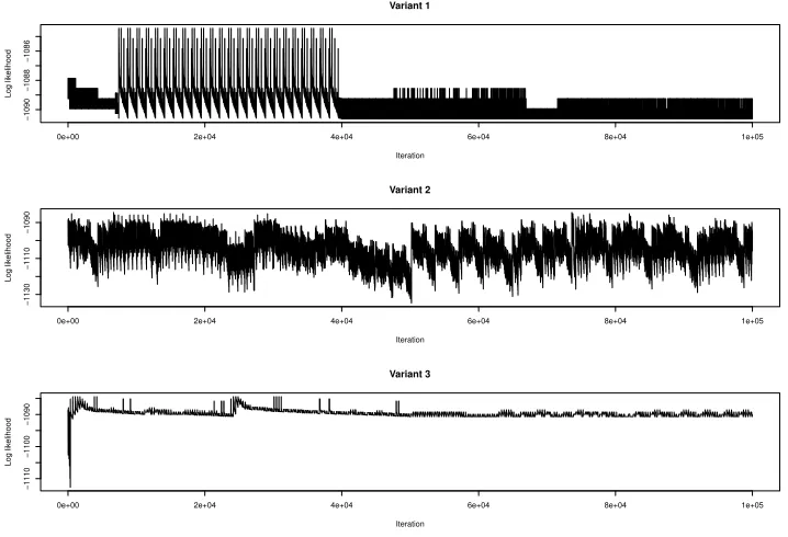
The third example we look at is a two generation dataset of the black tiger shrimp P. monodon (Jerry et al., 2005), downloaded from the FRANz software web site (Riester et al., 2009). The dataset from the website has profiles for 85 individual shrimp on seven loci. However for 10 shrimp the profiles are incomplete on some markers, and so these individuals were removed, leaving a dataset of 75 individuals. The FRANz software was used to generate estimates of allele frequencies. The three variants of Algorithm 4 were carried out to 100,000 iterations. (Curiously the same results were identical for with and without bounding, which might be because there are many pedigree having a likelihood close to the maximum, or perhaps simply because there are more individuals in this example compared to the others examined earlier. This is an issue that requires further exploration.) The trace plots are shown in Figure 5. Both Variant 1 and Variant 3 found 192 pedigrees having the highest likelihood value of -1084.44, whilstVariant 2found 3 such pedigrees. The next highest likelihood value found was -1085.14; this was found byVariant 1for 480 pedigrees and byVariant 3for 568 pedigrees, but for only 12 pedigrees
by Variant 2. Extending the number of iterations to 500,000 no additional
pedigrees having log-likelihood of -1084.44 were found by eitherVariant 1or
Variant 3, however the number of pedigrees found having a log-likelihood
of-1085.14 rose to 2856 forVariant 1and to 2824 forVariant 3.
0e+00 2e+04 4e+04 6e+04 8e+04 1e+05
−1090
−1088
−1086
Variant 1
Iteration
Log lik
elihood
0e+00 2e+04 4e+04 6e+04 8e+04 1e+05
−1130
−1110
−1090
Variant 2
Iteration
Log lik
elihood
0e+00 2e+04 4e+04 6e+04 8e+04 1e+05
−1110
−1100
−1090
Variant 3
Iteration
Log lik
[image:18.612.123.482.131.376.2]elihood
Figure 5: Successive pedigree log-likelihoods over 100,000 iterations, found for 75 individual black tiger shrimp using all algorithm variants, withVariant 3having a sort period of 350 iterations. Note the different scales on the likelihood axis.
highest log-likelihood of -1085.14. (By way of a timing comparison, each of the FRANz runs took approximately 3 seconds, whilst 100,000 iterations of the search algorithm took approximately 66 seconds on the same computer.)
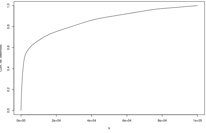
As we can see from Figure 5, the decay in the log-likelihood values is quite slow and not like the sharp decay exhibited in Figure 2. The cumulative relative likelihood of the pedigrees found byVariant 3of Figure 5, is plotted in Figure 6 where the likelihoods have been sorted from highest to lowest. Note that this is cumulative relative to the set of pedigrees found, not to the total likelihood of all possible pedigrees. The highest 1951 pedigrees found account for 50% of the total likelihood, the number rising to 69834 pedigrees to account for 95% of the total likelihood found.
5. Summary
0e+00 2e+04 4e+04 6e+04 8e+04 1e+05
0.0
0.2
0.4
0.6
0.8
1.0
k
Cum. rel. lik
[image:19.612.127.476.283.509.2]elihood
that pedigrees considered consecutively can have very different graphical struc-ture. This helps the search procedure to make large jumps in the pedigree space. In principle the algorithm generates all possible (positive likelihood) pedigrees without duplication, but in practice the space of pedigrees will usually be too large for an exhaustive search to be carried out.
Three variants of the algorithm were presented. In Variant 1 a priority queue is used to store the candidate pedigrees, and on each iteration the high-est likelihood candidate pedigree is selected from the queue. This generally performs quite well, but as illustrated in Figure 4 can take many iterations before finding a maximum likelihood pedigree. In Variant 2 the candidate pedigrees are stored in a first-in-first-out queue, which means that a wider va-riety of partitions is explored. This appears to be more efficient at finding a highest likelihood pedigree quite early, however there is wide variability in the likelihoods of pedigrees in successive iterations. A third variant was also exam-ined, in which candidate pedigrees are stored in a first-in-first-out queue, but periodically the queue is sorted so that high-likelihood pedigrees are at the front of the queue. Note that if the sorting period is set to 1, then this reduces to
Variant 1, and if the sorting period is set to be larger than the pre-set number
of iterations to be carried out, then this reduces to Variant 2. This seemed to perform the best, though the behaviour will depend on the choice of sorting period. It is planned to explore this issue further elsewhere. A bounding proce-dure was described, but it appears this might be effective only for a low number of individuals; again this is an issue that will be explored elsewhere.
There are various extensions that could be considered. One is to use the set of pedigrees found during a search in a pedigree averaging procedure. Indeed, this was the main motivation for developing the algorithm. Although a maximum likelihood pedigree will contain many features in common with the true pedigree, averaging over a set of high-likelihood pedigrees will take account of pedigree uncertainty. For example one could look at how often a particular feature in a pedigree, for example a particular individual i has a particular parent j, and using the pedigree likelihoods find the posterior probability of such a parent child combination (assuming, say, a uniform prior over the two possibilities ofj
is a parent ofi, andj is not a parent ofi).
search algorithms. However, such structural priors could be straightforwardly combined with the set of pedigrees found after the likelihood based search pro-cedure of this paper. Alternatively, and probably better, candidate pedigrees could be found using the likelihood search of Algorithm 4, and then combined with structural prior information (and so adjusting the P.valuescore) before being placed inQueue. In this way the search will be more focussed on the high posterior pedigrees of interest rather than high likelihood pedigrees; this is an area for further research.
References
Almudevar, A., 2003. A simulated annealing algorithm for maximum likelihood pedigree reconstruction. Theoretical Population Biology 63, 63–75.
Almudevar, A., LaCombe, J., 2012. On the choice of prior density for the Bayesian analysis of pedigree structure. Theoretical Population Biology 81, 131–143.
Blouin, M. S., 2003. DNA-based methods for pedigree reconstruction and kin-ship analysis in natural populations. TRENDS in Ecology and Evolution 18 (10), 503–511.
Cowell, R. G., 2009. Efficient maximum likelihood pedigree reconstruction. The-oretical Population Biology 76, 285–291.
Cussens, J., 2010. Maximum likelihood pedigree reconstruction using integer programming. In: In Proceedings of the Workshop on Constraint Based Meth-ods for Bioinformatics (WCB-10) Edinburgh.
Cussens, J., Bartlett, M., Jones, E. M., Sheehan, N. A., 2012. Maximum likeli-hood pedigree reconstruction using integer linear programming. Genetic Epi-demiology, (submitted and under review).
Egeland, T., Mostad, P. F., Mev˚ag, B., Stenersen, M., 2000. Beyond tradi-tional paternity and identification cases: Selecting the most probable pedi-gree. Forensic Science International 110, 47–59.
Gill, P., Ivanov, P. L., Kimpton, C., Piercy, R., Benson, N., Tully, G., Evett, I., Hagelberg, E., Sullivan, K., 1994. Identification of the remains of the Romanov family by DNA analysis. Nature Genetics 6, 130–135.
Jerry, D. R., Evansa, B. S., Kenway, M., Wilson, K., 2005. Development of a microsatellite DNA parentage marker suite for black tiger shrimp penaeus monodon. Aquaculture 255, 1–4.
Kruskal, J. B., February 1956. On the shortest spanning subtree of a graph and the traveling salesman problem. Proceedings of the American Mathematical Society 7 (1), 48–50.
Lawler, E., 1972. A procedure for computing the K best solutions to discrete optimization problems and its application to the shortest path. Management Science 7, 401–405.
Murty, K. G., 1968. An algorithm for ranking all the assignments in order of increasing cost. Operations Research 16 (3), 682–687.
Nilsson, D., June 1998. An efficient algorithm for finding theM most probable configurations in a probabilistic expert system. Statistics and Computing 8, 159–173.
Pemberton, J. M., 2008. Wild pedigrees: the way forward. Proceedings of the Royal Society, Series B 275, 613–621.
Riester, M., Stadler, P. F., Klemm, K., 2009. FRANz: Fast reconstruction of wild pedigrees. Bioinformatics 25, 2134–2139.
Sheehan, N. A., Egeland, T., Jul 2007. Structured incorporation of prior in-formation in relationship identification problems. Annals of Human Genetics 71 (Pt 4), 501–518.
URLhttp://dx.doi.org/10.1111/j.1469-1809.2006.00345.x
Silander, T., Myllym¨akki, P., 2006. A simple approach to finding the glob-ally optimal Bayesian network structure. In: Dechter, R., Richardson, T. (Eds.), Proceedings of the 22nd Conference on Artificial intelligence (UAI
2006). AUAI Press, pp. 445–452.
S¨orensen, K., Janssens, G. K., 2005. An algorithm to generate all spanning trees of a graph in order of increasing cost. Pesquisa Operacional 25 (2), 219–229.
Thompson, E. A., 1976. Inference of genealogical structure. Social Science In-formation sur les Sciences Social 15, 477–526.
Thompson, E. A., 1986. Pedigree Analysis in Human Genetics. John Hopkins University Press, Baltimore.