A Method for Designing Efficient Routes for Home Healthcare Agencies Considering Uncertain Future Demand

(1)

Rochester Institute of Technology

RIT Scholar Works

Theses Thesis/Dissertation Collections

7-19-2012

A Method for Designing Efficient Routes for Home

Healthcare Agencies Considering Uncertain Future

Demand

Nisha Nataraj

Follow this and additional works at:http://scholarworks.rit.edu/theses

This Thesis is brought to you for free and open access by the Thesis/Dissertation Collections at RIT Scholar Works. It has been accepted for inclusion in Theses by an authorized administrator of RIT Scholar Works. For more information, please [email protected].

Recommended Citation

(2)

Rochester Institute of Technology

A METHOD FOR DESIGNING EFFICIENT ROUTES

FOR HOME HEALTHCARE AGENCIES

CONSIDERING UNCERTAIN FUTURE DEMAND

A Thesis

Submitted in partial fulfillment of the requirements for the degree of

Master of Science in Industrial Engineering

in the

Department of Industrial & Systems Engineering Kate Gleason College of Engineering

by Nisha Nataraj

(3)

DEPARTMENT OF INDUSTRIAL AND SYSTEMS ENGINEERING

KATE GLEASON COLLEGE OF ENGINEERING

ROCHESTER INSTITUTE OF TECHNOLOGY

ROCHESTER, NEW YORK

CERTIFICATE OF APPROVAL

M.S. DEGREE THESIS

The M.S. Degree Thesis of Nisha Nataraj

has been examined and approved by the

thesis committee as satisfactory for the

thesis requirement for the

Master of Science degree

Approved by:

____________________________________ Dr. Mike R. Hewitt, Thesis Advisor

(4)

DEDICATION

To my parents, for their ever-patient support and for believing in me when I didn’t. To my

grandparents, for showing me that hard work always has its rewards, even when the fruit is not

(5)

ACKNOWLEDGMENT

This thesis, and all the lessons learned along the way, would not have been possible without my

advisor, Dr. Mike Hewitt. I am especially grateful for his constant guidance, encouragement and

faith. Understanding and interpreting data is a difficult skill, but his ever-present curiosity and

keen interest has been a valuable lesson, something I will treasure for the rest of my graduate

life. I know that all the hours spent reviewing my work could not have been easy, but his patient

attention to detail has taught me that we can always do better – the end result is always so much

more satisfying. Thursday afternoons will forever remind me that research can be fun.

I would like to thank Dr. Michael Kuhl for taking the time and effort to be on my thesis

committee. His feedback, always prompt, has taught me the value of perspective and to never

lose sight of the bigger picture. I am indebted to both Dr. Hewitt and Dr. Kuhl for encouraging

me to continue on with my graduate studies and giving me the advice needed to do so.

I owe much to the Industrial and Systems Engineering department. I am obliged to both

the people and the resources needed for me to work on my research and successfully complete

my thesis.

Every graduate student has that task in front of them that seems at one point

insurmountable; their Everest. I will be forever grateful to my sister-in-law, Namitha, and close

friend, Suraj, for spending all those hours patiently answering my programming questions, but

more so, for instilling in me the belief that I could learn to code. The CS tutoring lab was a great

(6)

I can never completely thank my family, my parents and my brother, Nakul, enough for

their unconditional love and support. Last, but far from the least, I would like to express my

deepest gratitude to Tejas. His patient love and understanding has given me the strength to face

(7)

ABSTRACT

Faced with increasing demand for home health care that is rising faster than the supply of

resources needed to deliver it and drastic budget cuts, many home care agencies are struggling to

remain operational. There is a need for efficient routing that doesn’t compromise on the quality

of care achieved when a patient is visited by the same nurse over the entire period of care, also

known as care-giver continuity or continuity of care. Because care periods often last more than

60 days, care-giver continuity causes scheduling decisions to have a long-term impact by

potentially restricting the agency from making alternative assignments that could reduce routing

costs. Our research aims to understand and quantify the benefit of utilizing time horizons of

60-90 days when making routing decisions under the constraint of continuity of care. We do so by

defining the Home Health Care Routing Problem (HHCRP) as a variant of the Vehicle Routing

Problem (VRP), known as the Consistent VRP, that includes the continuity of care requirement.

Unlike related literature on this problem which considers planning horizons of at most a week,

computational experiments in a variety of settings suggest the importance of considering

planning horizons of 2-3 months when developing schedules for care-givers. Given that it is

almost impossible to have complete information about future patients that far ahead, we also

present a method that enables planners to design schedules for care-givers in the face of such

(8)

LIST OF TABLES AND FIGURES

Table 1 - Length of planning horizon considered in the literature ... 18

Table 2 - Instance Details ... 35

Table 3 – Savings in travel time from comparing WBW and LTP planning strategies ... 37

Table 4 - Number of nurses: WBW v/s. LTP ... 38

Table 5 - Average number of patients seen per nurse per day: WBW v/s. LTP ... 38

Table 6 – Savings in travel time from comparing WBW, LTP and DLTP strategies ... 41

Table 7 - Number of nurses, comparing WBW, LTP and DLTP strategies ... 42

Table 8 - Average number of patients seen per nurse per day, comparing WBW, LTP and DLTP strategies ... 43

Table 9 - Week we start to see savings ... 44

Table 10- Average Computational Times ... 44

Table 11 - Time taken to find best solution ... 45

Table 12 - Instances for experiments with reduced visit times ... 45

Table 13 – Comparison of 30 minute versus 60 minute visit times... 46

Table 14 - Average number of patients seen per nurse per day: 30 minute versus 60 minute visit times ... 47

Table 15 – Steady demand experiment instances ... 48

Table 16 – Savings in travel time for steady-demand experiments: WBW v/s. DLTP ... 49

Table 17 – Average number of patients seen per nurse per day, steady demand experiments ... 50

Table 18 – Number of nurses in the steady demand experiments: WBW v/s. DLTP ... 50

Table 19 - Savings in travel time from comparing WBW, DLTP and DLTP (UI) strategies ... 56

(11)

Table 21 - Average number of patients seen per nurse per day for WBW, DLTP and DLTP (UI)

strategies ... 56

Table 22 – Comparison of savings in travel time for DLTP (UI): 30 minute v/s. 60 minute visit times ... 57

Table 23 – Number of Nurses for DLTP (UI): 30 minute v/s. 60 minute visit times ... 57

Table 24 - Average number of patients seen per day for DLTP (UI): 30 minute v/s. 60 minute visit times ... 58

Table 25 - Magnitude of weekly savings in hours WBW v/s. LTP – Growing Demand ... 69

Table 26 - Magnitude of weekly savings in hours WBW v/s. DLTP – Growing Demand ... 69

Table 27- Magnitude of weekly savings in hours WBW v/s. DLTP – Steady Demand... 70

Table 28 - Magnitude of weekly savings in hours WBW v/s. DLTP (UI) – Steady Demand ... 70

Figure 1 - Process of scheduling a visit for a new patient at a typical agency ... 5

Figure 2 - Search operators used in the ConRTR algorithm (Gröer et al., 2008) ... 20

Figure 3 – Deriving daily routes from template routes in the ConRTR ... 25

Figure 4 - Week by Week Planning ... 32

Figure 5 - Long-term Template Planning ... 32

Figure 6 - Factors and Levels for Experimental Design ... 33

Figure 7 - Average weekly value-added utilization for a sample rural setting with 400 initial patients over an 8 week horizon. ... 39

(12)

Figure 9 - Average weekly utilization for a sample rural setting with 200 initial patients over an 8

week horizon in a steady demand experiment ... 49

Figure 10 – Discounted Long-term Template Plan with Uncertain Information... 52

(13)

1. INTRODUCTION

A study conducted by the National Association for Home Care and Hospice (NAHC, 2006)

showed that in 2006, home health care workers drove close to 5 billion miles in the United

States. As of 2008, there were approximately 958,000 home health employees across the country

(NAHC, 2010).Home Care refers to the care provided by skilled and non-skilled care-givers for

patients, typically homebound, within their own homes. There are a wide range of services

available for in-home care, ranging from hospice care to wound and pain management. Patients

are typically recommended home health care by their primary physician or after discharge from a

hospital. The episode of care often lasts 60-90 days, during which time most individuals need to

be visited multiple times each week by their care-givers.

In-home care is an attractive alternative to nursing homes and hospitals because of lower

costs and improved quality of life benefits. For example, the average in-home management cost

for ventilator-dependent adults on a daily basis was only $235 in the year 1992, whereas the

associated daily cost when hospitalized was $719 (Bach, Intintola, Alba, & Holland, 1992).

Lower costs can also enable patients to be seen for longer periods of time in turn resulting in the

better management of conditions. Some quality of life benefits are that patients can live in the

comfort of their own homes and have the option of assistance with routine self-care activities

such as feeding, bathing and cleaning.Home care has also been found to reduce the likelihood of

re-admission, not only improving quality of life, but saving money as well. One such example is

a study on psychiatric patients in Connecticut that determined that 46% of those that were

hospitalized without first participating in the in-home crisis intervention program were

subsequently re-admitted after their discharge, compared to a readmission rate of only 12% for

(14)

Home Health Care (HHC) is a growing industry. In 2008, around 33,000 care-givers

made visits to approximately 12 million patients across the country (NAHC, 2010). In spite of

the large demand for home care, agencies have been struggling to stay afloat. According to a

report released by the Home Care Association (HCA) of New York and the New York

Association for Homes and Services for the Aging (NYAHSA), since 2008 , Medicaid home

services has lost over $430 million in budget cuts, (NYAHSA & HCA, 2011). To make

matters worse, more than 70% of agencies were reported to be operating at a loss in 2008.

These large scale operations suggest that gasoline costs can have a significant impact on the economics of home health care. With worsening operating losses, high fuel costs and bleak financial scenarios, it is critical for agencies to reduce transportation costs associated with

making visits to patients’ homes.

However, the need for efficient routing goes beyond agencies’ current financial state of

affairs. Efficient routes not only reduce costs but also allow care givers to spend more time at

patients’ homes and reduce non-value-added travel time. Furthermore, agencies can

accordingly plan for anticipated staffing requirements ahead of time. A study on the benefits of

the implementation of a Decision Support System for scheduling in home care organizations in

Sweden found reduced short-term sick leave amongst nurses and a reduction in the number of

missed visits (Eveborn et al., 2009). In addition, organization managers reported better staffing

and budgetary control.

Other challenges that agencies currently face is that schedulers typically use relatively

unsophisticated planning systems to design routes for nurses. As a result, planning is done for a

single patient at a time, on-demand, and as we discovered during interviews at a large local

(15)

Therefore, at the end of the day, it is clear that efficient routes have a far reaching impact that

transcends monetary benefits.

An important quality of care metric in home health is continuity of care. With continuity

of care, patients are always seen by the same care-giver, resulting in saved time and effort

associated with familiarizing new care-givers with patients’ histories and care plans, as well as

fostering close relationships and trust between patients and their care givers. Continuity also

has other benefits. In the meta-analysis by Cabana & Jee (2004) in a general health-care

setting, the authors found that continuity of care over time resulted in reduced hospitalizations,

improved patient satisfaction and improved receipt of preventive services such as

mammograms and MMR vaccinations. One challenge that maintaining high levels of

continuity of care presents to agencies is that once a care-giver (henceforth referred to as a

nurse) is assigned to a patient, that assignment should remain fixed for the remainder of the

care period. With periods of care typically lasting 2-3 months, this means that the scheduling

decisions made by an agency have a long-term impact on their daily costs. However, agencies

rarely consider this long-term impact when making scheduling decisions and research related

to the scheduling problem faced by home health care agencies rarely considers planning

horizons longer than one week.

Based on interviews with schedulers at a large local home health care agency, Figure 1

shows the typical process of scheduling patients at a large local home health care agency.

Referrals from hospitals and other sources are built into the database of the scheduling system.

Each patient is then assessed during an initial visit to determine the kind and frequency of care

that is required. Once the evaluation is complete, the internal staff then filter the visit requests

(16)

therapist or some other skilled/unskilled care-provider. Schedules and assignments are created

regularly (ensuring that the number of visits for each patient is at least as good as the compliance

standards) and updated throughout the week as changes are made. As mentioned earlier, a patient

often needs to be seen multiple times a week. The frequency and days on which a patient needs

to be seen are usually pre-determined, and stay fixed for remainder of the care period (for

example, a patient may need to be seen three days a week, on Mondays, Wednesdays and

Fridays for 60 days). In spite of the availability of scheduling software, we found that the

planners often choose to design schedules manually. While this is a cumbersome process in

itself, the added difficulty of keeping track of continuity of care requirements makes it even

harder. The nurse then makes the visit, and the planners schedule the next visit. The cycle repeats

until the end of the episode of care. Highlighted in Figure 1, is the stage of the scheduling

process that can be automated with an algorithm that produces daily routes for nurses. On

occasion, changes may need to be made after a schedule has already been created. For example,

a nurse might call in sick or a patient might request a change in schedule. However, we consider

(17)

[image:17.612.97.533.73.338.2]

Figure 1 - Process of scheduling a visit for a new patient

In this research we computationally demonstrate the benefits of considering long

planning horizons (2-3 months) when maintaining high levels of continuity of care. We

modeling the scheduling problem faced by home health care agencies as a type of Vehicle

Routing Problem (VRP), called the Home Health Care Routing Problem (HHCRP). Our first

experiments focus on a deterministic setting, where all patients to be se

horizon are known. However, with planning horizons of this length, such an assumption is

clearly unrealistic. Thus, we next present a method that, when executed in a rolling

manner, anticipates future patients requiring care

Because many agencies are small and have unsophisticated information systems, we designed

this method to have low data requirements to capture uncertainty.

The rest of the thesis is organized as follows:

Process of scheduling a visit for a new patient at a typical agency

computationally demonstrate the benefits of considering long

3 months) when maintaining high levels of continuity of care. We

experiments focus on a deterministic setting, where all patients to be seen during the planning

clearly unrealistic. Thus, we next present a method that, when executed in a rolling

manner, anticipates future patients requiring care while assigning known patients to nurses.

this method to have low data requirements to capture uncertainty.

is organized as follows: We first formally define the problem at a typical agency

computationally demonstrate the benefits of considering long

3 months) when maintaining high levels of continuity of care. We do so by

en during the planning

clearly unrealistic. Thus, we next present a method that, when executed in a rolling-horizon

while assigning known patients to nurses.

(18)

discussing the different VRP variants relevant to the HHCRP and previous work in home health

care routing. A background of the Consistent Record to Record algorithm designed by Groer,

Golden, & Wasil (2008) is provided, followed by a description of its adaptation to the home

health care setting. We then describe our experimental design and describe two planning

strategies that are central to establishing the impact of long-term continuity. Following this, we

present an enhancement of the Consistent Record to Record algorithm for when long planning

horizons are considered and a variant of the method that recognizes uncertainty with respect to

(19)

2. PROBLEM STATEMENT

In this section, we discuss the objectives of this research and then formally define the HHCRP

followed by a Mixed Integer Program (MIP) formulation of the problem to provide a precise

mathematical definition of the objective and constraints of the problem.

2.1.Objectives

The goal of this research is to determine the importance of considering long planning horizons

when developing schedules for nurses in a home health care setting where continuity of care is a

critical quality metric. At present, most agencies plan “on-demand”, typically considering each

patient as they come, on a case-by-case basis. Furthermore, previous literature in the home health

care and vehicle routing settings rarely consider planning horizons that are longer than a week.

This research emphasizes the benefits achieved from planning horizons that are 2-3 months long.

The specific objectives for this research are:

1. To understand the routing costs and staffing requirements of planning over weekly basis

when compared with a long-term planning horizon over the duration of 2-3 months using a

routing method that is adapted to the home health care setting;

2. To develop a method that can handle fluctuation in the number of patients over a planning

horizon of 2-3 months and demonstrate its capabilities in scenarios with growing demand and

steady demand;

3. To develop a method for long-term planning which anticipates future patients and has low

data requirements to model uncertainty; and

(20)

The results of this research will enable home health care agencies to design more efficient

routes and anticipate staffing needs ahead of time. Efficient routes will also allow nurses to have

more time to spend with their patients. The anticipated impact of this research can also apply to

other routing environments, such as package delivery, where consistency is a desired metric. By

quantifying the benefits achieved from long-term planning, we emphasize the underlying need

for routing methods that are designed for longer planning horizons.

2.2. Problem Description

The HHCRP is defined on a graph on which the agency and patient homes are represented as

nodes, and routes connecting these nodes are represented as arcs. Nurses set out from either their

homes or the agency at the beginning of the day and visit those patients who need to be seen for

that day. Patients require multiple visits over a planning horizon of 60-90 days. The days that a

patient requires visits and the frequency of these visits are assumed to be fixed beforehand. A

realistic assumption based on our conversation with the agency is that the frequency and days of

visit are determined in advance based on the type of care needed, so that it is mutually acceptable

to both the patient and the agency. Once a visit schedule and frequency are decided, it stays fixed

for the remainder of the patient’s episode of care. For example, a patient may need to be seen

twice a week, every Monday and Thursday for the next 8 weeks.

We make some assumptions about the problem. First, we do not differentiate patients

based on condition, or nurses based on skill/qualifications. Many agencies work with home

health aides who assist with routine self-care and hospice care, and agencies typically do not

differentiate aides based on skill/qualifications. Second, the number of nurses is not a fixed input

(21)

economical routing decision cannot be made without exceeding the maximum number of hours

that existing nurses may work on a given day. In a realistic setting, agencies often have the

option of outsourcing to third-party providers during periods of high demand.

2.3. Mathematical Model

The sets used in the formulation of the MIP and the subsequent algorithm are defined as follows

– N is a set of nurses that need to visit the set of all patients, P over a horizon, D. P` is a subset of

the set P, and includes all patients that need visits, but excludes the agency/depot. In order for a

route to be feasible, the total time that a nurse works on a given day, d, must be at most T.

Let cij represent the cost associated with traveling from node i to node j. The parameter

wid is considered to be 1 if a patient i requires a visit on day d. Let aid be the arrival time at

patient i on day d. The parameter sid is the service or visit time for each patient i. We define the

decision variable xijnd to be 1 if a nurse n travels from node i to node j on day d and 0 otherwise.

The decision variable yind is considered to be 1 if a nurse n visits a patient i on day d and 0

otherwise. Finally, the notation o represents the depot or agency from which a nurse may start

his/her day.

∑∑∑∑ (1)

s.t.

∑ = 1 ∀ ∈ , ∀ ∈ (2)

∑ = 1 ∀ ∈ , ∀ ∈ (3)

∑ = ∀ ∈ ′, ∀ ∈ (4)

∑ = ∀ ∈ , ∀ ∈ , ∀ ∈ (5a)

(22)

_!+ _# − 2 ≤ _! − _#≤ −(_!+ _#− 2) (6)

∀ )* _!) _#, + ≠ -, ∀ ∈ , ∀ ∈

)+ .*+ /0 − .1 − 01 ≤ ) (7)

∀ ∈ , ∀ ∈ ′, ∀ ∈ , ∀ ∈

)+ .*+ /0 + .1 − 01 ≥ ) (8)

∀ ∈ , ∀ ∈ ′, ∀ ∈ , ∀ ∈

∑, ≤ |4| − 1 (9)

567 4 ⊆ , /ℎ 2 ≤ |4| ≤ , ∀ ∈ , ∀ ∈

0 ≤ )+ (*+ /) ≤ 1 ∀ ∈ ′ (10)

∈ ;0,1<; ∈ ;0,1<; ) ≥ 0; (11)

∀ ∈ , ∀ ∈ , ∀ ∈ , ∀ ∈

The objective (1) of the HHCRP is to minimize the total cost (or equivalently, the total

distance) of all routes for all nurses over all days in the horizon. Constraints (2) and (3) make

sure that a nurse starts and ends his/her day from the depot. Constraint (4) ensures that nurses

visit patients on each day that they require a visit and do so at most once. Each patient has just a

single successor and predecessor as ensured by (5a, 5b). Constraint (6) ensures that the same

nurse visits a patient when multiple visits are required. Constraints (7) and (8) determine the

arrival time at a patient’s home. Sub-tours are eliminated with constraint (9). Finally, (10)

imposes restrictions on the maximum time that a nurse may work on a given day.

While we formulate the problem as an MIP, we cannot solve it as such. This is because

typically MIPs are used for smaller problems with fewer nodes, say, around 100 patients.

(23)

significantly increasing the size of the problem by considering a planning horizon of 2-3 months.

Because current solvers cannot solve these problems in realistic run-times, we instead choose to

(24)

3. RELATED WORK

In this section we first present an overview of the Vehicle Routing Problem and its variants that

are relevant to the HHCRP, followed by a review of some work that has been carried out in the

home care routing setting.

3.1. The Vehicle Routing Problem

The Vehicle Routing Problem was first introduced in 1959 by Dantzig and Ramser as the Truck

Dispatching Problem (Dantzig & Ramser, 1959). The objective was to develop the shortest

possible set of routes for a fleet of gasoline trucks to deliver gasoline from a major terminal to

several smaller stations. It has since spawned a class of problems encompassing different

applications ranging from emergency services to home delivery, while dealing with a variety of

constraints such as capacity, time windows, dynamic requests, etc.

Many practical instances of the VRP involve problem sizes that consider up to several

thousand customers (Kytojoki, Nuortio, Braysy, & Gendreau, 2007; Li, Golden, & Wasil, 2004)

and cannot be solved to optimality in realistic runtimes. Baldacci, Mingozzi, & Roberti (2011)

provide a review of recent exact algorithms that have been developed for the Capacitated VRP

(CVRP) and VRP with Time Windows (VRPTW) variants. Currently, exact algorithms are

capable of solving instances with at most a few hundred customers in a single day planning

horizon whereas home care agencies often see a few thousand patients a week. For larger

problems, the focus has been on developing classical heuristics and meta-heuristics that solve the

problem to near-optimality in shorter times. Local search heuristics tend to have a comparatively

(25)

search space better by allowing worsening solutions. A review of these is available in Laporte,

Gendreau, Potvin, & Semet (2000).

3.2. Variants of the VRP

The HHCRP is often modeled as a variant of the VRP (Cheng & Rich, 1998; Steeg & Schröder,

2008). In the HHCRP, each nurse’s schedule for the day is identified by a route and patients by their locations. Both problems also include a service or visit time associated with each visit.

Additionally, there is a restriction on maximum length of day (that includes both travel and

service times) for drivers and nurses. Several variants of the VRP focus on issues that are

important in the context of home health such as having multiple depots (for nurses to have the

option of starting their day from their own homes), periodicity (because patients often require

multiple visits), and consistency (which translates to continuity of care in the home health

setting).

In the HHCRP, patients need to be visited periodically throughout their episode of care.

For example, a patient might need physical therapy three times a week for two months. The

Periodic VRP (PVRP) considers a planning horizon of several days, such as a week. Customers

often need to be visited more than once during the planning horizon. The PVRP has been

previously applied to grocery distribution, waste collection, etc., and a review of these

applications is available in Francis, Smilowitz, & Tzur (2008). A Variable Neighborhood

Search (VNS) is used in Hemmelmayr, Doerner, & Hartl (2009) and Pirkwieser & Raidl (2008)

to solve the PVRP. VNS, first presented in Mladenovic & Hansen (1997) is a Meta-heuristic that

explores increasingly distant neighborhoods of the current solution using search operators and

(26)

The Consistent VRP (ConVRP), first described by Gröer et al. (2008) aims to design

routes that ensure that a customer is visited by the same driver/vehicle each time he or she

requires a visit. The ConVRP is inherently periodic because it considers a time frame during

which a customer has to be visited multiple times by the same driver. While the majority of their

analysis is based on a horizon of only a single week, they also conducted some tests on a

real-world instance spanning 5-weeks, using 4 weeks of template routes to derive routes for the fifth

week. From a VRP modeling standpoint, driver consistency is equivalent to continuity of care

within a home health care setting. The authors were one of the first to focus exclusively on

consistency and did so in the small package shipping industry. Other papers (Smilowitz, Nowak,

& Jiang, 2011; Zhong, Hall, & Dessouky, 2007) have previously looked at driver familiarity,

which is a variation of consistency. With driver familiarity, if a driver repeatedly visits a

particular region, he/she will know the routes better and as a result, delivery performance

improves. This work can be applied in the small package delivery industry where it is important

for drivers to know their way around a region well in order to find addresses quickly.

Real-life applications of the VRP often have several sources of uncertainty. Taking them

into consideration makes methods more likely to produce solutions that are robust with respect to

different realizations of uncertain parameters. When considering extremely long planning

horizons in the VRP or home health care setting, it is unlikely that every patient who needs a

visit in future weeks is known ahead of time. Incorporating this uncertainty into the planning

process may yield better routes.

There are typically two methods for incorporating stochastic information into a VRP –

one option is to model it as a Chance Constrained Program (CCP), and the other is to model it as

(27)

is a minimum expected level of success. However, this method does not consider the cost of

recourse action (such as returning to the depot to restock in case of exceeded capacity or

skipping absent customers) if the routes fail. SPRs, on the other hand, try to minimize the

expected cost of the routes as well as the cost of recourse actions. The review by Gendreau,

Laporte, & Seguin (1996a) provides a good overview of the stochastic VRP and its variants.

The different sources of uncertainty typically considered in an SVRP include demand,

customers, and travel times. In VRPs with stochastic demands, customer locations are

deterministic; however, demands are unknown and are realized only once the vehicle arrives at

the location. On the other hand, with stochastic customers, demands are deterministic, but

customer locations and arrival times are not known before hand. Flatberg, Hasle, Kloster,

Nilssen, & Riise (2005) review the existing literature in the stochastic VRP, including the SVRP

with travel times. Some papers also consider the combined effect of stochastic demand and

customers (Gendreau, Laporte, & Seguin, 1995; Gendreau, Laporte, & Seguin, 1996b). In the first paper, the authors use an integer-L shaped algorithm to solve the VRP with Stochastic

Demands and Customers (VRPSCD) exactly, observing that stochastic customers make the

problem harder. In the second paper, the authors develop the TABUSTOCH algorithm to solve

the VRPSCD and compare it against the optimal solution obtained from the integer-L shaped

algorithm.

From the point of view of the HHCRP, because patients are not associated with any sort

of “demand”, the largest source of uncertainty is customers. With the VRPSC, typically, the set

of customers who can potentially make a request is known ahead of time. However, some of

these customers may not need to be visited, because of which the recourse action involves just

(28)

Gendreau, Laporte, Seguin (1996). In Bent & Van Hentenryck (2004), the authors propose a

Multiple-Scenario Approach to solve the partially dynamic VRPTW with Stochastic Customers.

The paper exploits stochastic information about dynamic customers by creating a projected plan

with predicted customers in order to improve the quality of the solution. A consensus function

then chooses the most similar plan from multiple plans that contain both static (known) and

dynamic requests.

Campbell & Savelsbergh (2005) define the Home-Delivery Problem (HDP) for grocery

delivery with stochastic customers. The goal is to be able to visit as many customers as possible

while maximizing the total profit from these visits. The authors compare different

profitability-based insertion heuristics to create a set of routes that will help evaluate whether to accept or

reject incoming customer requests. There has not been much work done as yet in stochastic and

dynamic home care routing. However, Bennett & Erera (2011) study a dynamic home health care

routing and scheduling problem for a single-nurse variant where all patient requests are not

known in advance. The authors consider a rolling horizon of a year and handle requests for new

patients as they arrive. They achieve this by developing distance and capacity-based

insertion heuristics with an objective of maximizing the number of patients seen. This is

one of the only few papers available in the literature to consider a planning horizon that far

out in a home health setting.

3.3. Home health care routing

In comparison to the literature available on the VRP, there has been relatively little work done in

the HHCRP. Kergosien, Lenté, & Billaut (2009) model the home health care problem as a

multiple-Traveling Salesman Problem (m-TSP) with a slight variant of continuity, in that some

(29)

constraint. The problem is formulated as an Integer Linear Program (ILP) and solves instances

with up to 40 locations to optimality. Cheng & Rich (1998) also formulate the HHCRP as an

MIP. A nurse routing component is integrated into a Spatial Decision Support System in Begur,

Miller, & Weaver (1997) along with a Geographical Information System (GIS) to aid

schedule-making. The authors use the sequential Clark & Wright savings algorithm to assign routes to

nurses and a Nearest Neighbor heuristic to improve these individual routes. Two papers, (Bertels

& Fahle, 2006; Steeg & Schröder, 2008) use a hybrid of Constraint Programming (CP) and a

meta-heuristic to solve the HHCRP. The latter considers the idea of continuity of care by trying

to minimize the number of different nurses that visit a single patient. In the paper by Eveborn,

Flisberg, & Rönnqvist (2006) the authors build a decision support system, LAPS CARE, for

Swedish home care organizations. The problem is formulated as a set partitioning model and

solved using a repeated matching heuristic. They incorporate the importance of continuous care

by using a weighted objective function. The LAPS CARE system is designed to create plans a

few days in advance and handle any last minute changes as necessary. The impact and numerous

benefits of LAPS CARE on the Swedish home care industry is well documented in Eveborn et

al. (2009).

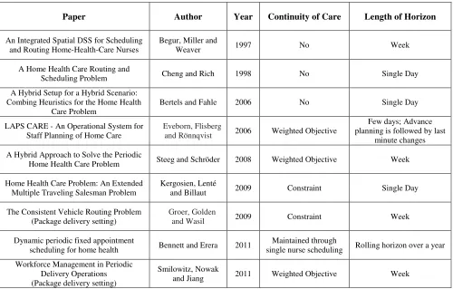
While models (and solution methods) have been presented for the HHCRP, it is not yet

known how they should be used. In particular, the combination of long periods of care and

continuity of care suggests that long planning horizons should be considered. We summarize in

Table 1 the length of the planning horizon used in previous VRP and HHCRP literature that

considers continuity of care in some capacity. We note that few (if any) approaches consider

planning horizons longer than a week.

(30)

Paper Author Year Continuity of Care Length of Horizon

An Integrated Spatial DSS for Scheduling and Routing Home-Health-Care Nurses

Begur, Miller and

Weaver 1997 No Week

A Home Health Care Routing and

Scheduling Problem Cheng and Rich 1998 No Single Day

A Hybrid Setup for a Hybrid Scenario: Combing Heuristics for the Home Health

Care Problem

Bertels and Fahle 2006 No Single Day

LAPS CARE - An Operational System for Staff Planning of Home Care

Eveborn, Flisberg

and Rönnqvist 2006 Weighted Objective

Few days; Advance planning is followed by last

minute changes

A Hybrid Approach to Solve the Periodic

Home Health Care Problem Steeg and Schröder 2008 Weighted Objective Week

Home Health Care Problem: An Extended Multiple Traveling Salesman Problem

Kergosien, Lenté

and Billaut 2009 Constraint Single Day

The Consistent Vehicle Routing Problem (Package delivery setting)

Groer, Golden

and Wasil 2009 Constraint Week

Dynamic periodic fixed appointment

scheduling for home health Bennett and Erera 2011

Maintained through

single nurse scheduling Rolling horizon over a year

Workforce Management in Periodic Delivery Operations (Package delivery setting)

Smilowitz, Nowak

[image:30.612.60.560.70.389.2]

and Jiang 2011 Weighted Objective Week

(31)

4. BUILDING CONSISTENT ROUTES: THE CONRTR IN A HOME

HEALTH SETTING

Our analysis of routing costs over long planning horizons uses the Consistent Record-to-Record

(ConRTR) Algorithm, which is capable of solving large VRP instances, with up to several

thousand customers (Gröer et al., 2008). The ConRTR can solve these large problems very

quickly while inherently maintaining continuity of care. The algorithm is designed to minimize

the total distance traveled over all the routes while treating consistency (continuity of care in our

context) as a constraint.

4.1. Background

To ensure that customers are always visited by the same driver, the ConRTR creates a set of

template routes for all customers with multiple requests over the planning horizon. The template

routes are not actually traversed by vehicles; rather, they work as a framework from which each

daily route may then be derived. By deriving each day’s routes from the templates, it is ensured

that each customer is always visited by the same driver. As mentioned earlier, in the VRP and

the home health care setting, a common restriction is the maximum allowable duration of a

driver or nurse’s day. Because the templates consider customers over the entire period and are

never implemented themselves, it is hard to determine what the bounds on the duration of a

driver’s day should be to produce feasible daily routes. The problem arises when the derived

daily routes are found to exceed the maximum allowable length of the day, because all customers

do not need to be seen every day. For example, the algorithm may design a template route for a

vehicle considering all customers over, say, a week. Because all customers do not need to be

visited every day, the duration of the template route will be greater than what is allowed on any

(32)

for a template route and prevent it from being exceeded. These bounds on the travel time are

frequently recalculated by deriving daily routes, and checking for feasibility.

The ConRTR algorithm (see Algorithm 1) starts with an initial solution of template

routes generated by the modified Clark and Wright algorithm and iteratively makes changes to

the solution using one point, two point and two opt move operators, as shown in Figure 2.

One-point moves change the position of a single node in the solution, and two-One-point moves swap the

positions of two nodes in the solution. Two-opt moves, however, remove and replace two edges

from the solution. A two-opt move may be either inter- or intra-route. The second stage of the

ConRTR is based on Record to Record algorithm developed by Li, Golden, & Wasil (2004)

which considers both “uphill” (non-improving) and “downhill” moves (improving) in the hope of

[image:32.612.76.542.400.638.2]

finding better template solutions.

(33)

Algorithm 1 – The Consistent Record to Record Algorithm (Gröer et al., 2008)

Input:

• A set, P, of patients, with their visit frequency and geographic location known,

• A set of nurses each with maximum total travel time T, and D days in a planning

horizon.

• C denotes the current set of template routes being considered

• F denotes the most recently generated set of template routes that is known to lead to

feasible routes for each day

• F* represents the set of template routes that leads to the lowest total travel time for the

D days.

• I is the number of iterations in the diversification phase,

• J is the maximum number of non-improving iterations allowed before returning a

solution,

• α represents a tolerance for the amount of deterioration allowed in the local search

• λ is a parameter used in the Clarke-and-Wright algorithm to quickly generate multiple

initial solutions.

• Given a set of template routes S, let f(S) represent the total travel time of all D routes if

they are feasible.

Ouput: Set of routes for all customers across all days in the horizon

1. Initialization

a) Set I = 30, J = 5, α_{= .01,}l = 1, and λ = {0.6, 1.0, 1.4}

(34)

c) Partition the set of N customers into two groups, G1 containing all customers requiring

service on two or more days and G2 containing all customers requiring service on only

one day.

d) Compute an expansion factor E = |G1|/µdaily where µdaily is the mean number of stops

required on each day and |N| is the number of customers in the template. Make an initial

estimate for the maximum capacity of the template routes by setting Qtemplate = Q × E =

Q0 and estimate the length of day of the template routes by setting Ttemplate =T/ √@ = T0.

e) For all customers in G1, set the demand amount and service time to be the mean values of

these quantities taken across all days that the customer needs a visit.

2. Create an initial set of template routes

a) Generate an initial set of template routes C for the customers in G1 using the modified

Clarke-and-Wright algorithm with parameter λ [l] and maximum travel time Ttemplate = T0.

b) For each day d, create routes by removing customers from C not requiring service on day

d and then inserting customers from G2 requiring service only on day d..

c) If the routes for all D days are feasible, set F = C, Qold = Qtemplate, Told = Ttemplate. Go to

Step 3.

d) If at least one route on the D days is not feasible, then calculate the mean capacity

violation (VQ) and the mean travel time violation (VT ) across all routes, and tighten the

template constraints by setting Qtemplate = Qtemplate – VQ/2 and Ttemplate = Ttemplate− VT /2.

Return to Step 2.a and try to generate a set of feasible template routes.

3. Diversification Phase: Modify the current feasible template routes C = F. If f(C) < f(F*), set

(35)

a) Set Record equal to the total travel time of all routes in the current template C. Set

Deviation = α × Record.

b) For i = 1 to I

i) Apply the one-point move, two-point move, and two-opt move with record-to-record

travel to the current template routes C. Accept any improving move and only those

deteriorating moves where the total travel time of all template routes is less than

Record+Deviation and all routes satisfy the template constraints.

4. Improvement Phase: Improve the current solution C. Set k = 0.

a) Apply the one-point move, two-point move, and two-opt move, accepting only improving

moves until no further improvements can be found.

b) Construct routes for each of the D days by applying the customer removal and insertion

procedures.

c) If the routes for all D days are feasible, set F = C. Compute the minimum slack amount

across all daily routes in terms of capacity (SQ) and travel time (ST). Relax the template

constraints by setting Qtemplate = Qtemplate + SQ /2 and Ttemplate = Ttemplate + ST /2. Go to Step

5.

d) If at least one route on the D days is not feasible, then compute the mean violation (VQ

and VT ) as in Step 2f and tighten the template constraints by setting Qtemplate = Qtemplate

−VQ /2 and Ttemplate = Ttemplate − VT /2. Set k = k + 1. If k < 5, continue to find feasible

improvements by returning to Step 4.a. Otherwise, return to the last known feasible

template, setting C = F and go to Step 5.

(36)

template. Otherwise, we have been unable to improve the current solution for J iterations, so

stop modifying the current template and go to Step 6.

6. Set l = l + 1 and return to Step 2 to generate a new initial solution if l ≤ 3. Otherwise, use the best set of template routes (F*) found during the search to generate the routes for each of the

D days and return.

4.2. ConRTR in a home care setting

In order to adapt the ConRTR to a home health care setting (see Algorithm 2), we make some

minor changes. The ConRTR partitions the set of all customers to be visited across a given

period into two groups – one set of customers need multiple visits in the period, and the other

need only a single visit. The first adaptation of the ConRTR eliminates the need for the latter,

because we make the fair assumption that patients requiring home care always need more than

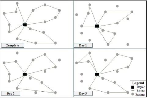
one visit over a horizon. Because of this, deriving daily routes is a simple matter of removing

patients who do not need to be seen on a given day as shown in Figure 3. However, in the

original ConRTR (Algorithm 1) there is an additional step that involves also adding patients who

need to be seen only once, since the issue of visit consistency does not arise for such patients.

The second adaptation concerns the demand and capacity associated with each customer and

vehicle in a typical package delivery setting. In the modified ConRTR, we remove any capacity

restrictions from the algorithm, because patients aren’t typically associated with “demands”.

The algorithm was coded in C++ using the classes and functions available in the open

(37)

[image:37.612.78.559.73.396.2]

Figure 3 – Deriving daily routes from template routes in the ConRTR. In this example we

planning period. The routes for each day are derived by removing patients who do not need to be seen on a given day from the template routes, depicted in the top left corner.

Algorithm 2 – The Modified Consistent Record to Record Algorithm Input:

• A set, P, of patients, with their visit frequency and geographic location known,

• A set of nurses each with maximum total travel time

horizon.

• C denotes the current set of t

• F denotes the most recently generated set of template routes that is known to lead to

feasible routes for each day

Deriving daily routes from template routes in the ConRTR. In this example we

planning period. The routes for each day are derived by removing patients who do not need to be seen on a given day from the template routes, depicted in the top left corner.

Consistent Record to Record Algorithm

of patients, with their visit frequency and geographic location known,

set of nurses each with maximum total travel time T, and D days in a planning

denotes the current set of template routes being considered

e most recently generated set of template routes that is known to lead to

easible routes for each day

Deriving daily routes from template routes in the ConRTR. In this example we assume a 3 day planning period. The routes for each day are derived by removing patients who do not need to be seen on a

of patients, with their visit frequency and geographic location known,

days in a planning

(38)

• F* represents the set of template routes that leads to the lowest total travel time for the

D days.

• I is the number of iterations in the diversification phase,

• J is the maximum number of non-improving iterations allowed before returning a

solution,

• α represents a tolerance for the amount of deterioration allowed in the local search

• λ is a parameter used in the Clarke-and-Wright algorithm to quickly generate multiple

initial solutions.

• Given a set of template routes S, let f(S) represent the total travel time of all D routes if

they are feasible.

Ouput: Set of routes for all patients across all days in the horizon

1. Initialization

a) Set I = 30, J = 5, α_{= .01,}l = 1, and λ = {0.6, 1.0, 1.4} as suggested in Gröer et al.,

(2008)

b) Set C = F = F* = ∅;

c) Compute an expansion factor E = |P|/µdaily where µdaily is the mean number of stops

required on each day and |P| is the number of patients in the template. Make an initial

estimate for the maximum length of day of the template routes by setting Ttemplate =T/ √@

= T0.

d) For all customers in P, set the service time to be the mean values of these quantities taken

across all days that the patient needs a visit.

(39)

a) Generate an initial set of template routes C for the patients in P using the modified

Clarke-and-Wright algorithm with parameter λ [l] and maximum travel time Ttemplate = T0.

b) For each day d, create routes by removing patients from C not requiring service on day d.

c) If the routes for all D days are feasible, set F = C, Told = Ttemplate. Go to Step 3.

d) If at least one route on the D days is not feasible, then calculate the mean travel time

violation (VT ) across all routes, and tighten the template constraints by setting Ttemplate =

Ttemplate− VT /2. Return to Step 2.a and try to generate a set of feasible template routes.

3. Diversification Phase: Modify the current feasible template routes C = F. If f(C) < f(F*), set

F* = C.

a) Set Record equal to the total travel time of all routes in the current template C. Set

Deviation = α × Record.

b) For i = 1 to I

i) Apply the one-point move, two-point move, and two-opt move with record-to-record

travel to the current template routes C. Accept any improving move and only those

deteriorating moves where the total travel time of all template routes is less than

Record+Deviation and all routes satisfy the template constraints.

4. Improvement Phase: Improve the current solution C. Set k = 0.

a) Apply the one-point move, two-point move, and two-opt move, accepting only improving

moves until no further improvements can be found.

b) Construct routes for each of the D days by applying the patient removal procedure.

c) If the routes for all D days are feasible, set F = C. Compute the minimum slack amount

across all daily routes in terms of travel time (ST). Relax the template constraints by

(40)

d) If at least one route on the D days is not feasible, then compute the mean violation ( VT )

as in Step 2.f and tighten the template constraints by setting Ttemplate = Ttemplate −VT /2. Set

k = k + 1. If k < 5, continue to find feasible improvements by returning to Step 4.a.

Otherwise, return to the last known feasible template, setting C = F and go to Step 5.

5. If f(C) < f(F*), set F* = C. If the objective function value of the current template routes C is less than Record, set j = 0. Set j = j+1. If j < J, return to Step 3 and continue modifying the

template. Otherwise, we have been unable to improve the current solution for J iterations, so

stop modifying the current template and go to Step 6.

6. Set l = l + 1 and return to Step 2 to generate a new initial solution if l ≤ 3. Otherwise, use the best set of template routes (F*) found during the search to generate the routes for each of the

(41)

5. COMPUTATIONAL ANALYSIS: IMPACT OF CONTINUITY ON

LONG-TERM PLANNING

In this section, we first present the planning strategies used to establish the impact of continuity

and then describe the tests performed on them in a variety of settings. Next, we present an

enhancement to the ConRTR that is designed for when the method is executed on problems with

long planning horizons and show its efficacy computationally.

5.1. Planning strategies

We consider two planning strategies to understand the long-term impact of continuity. Both these

strategies are implemented using the ConRTR. The first is a Week By Week planning strategy

(WBW) typically suggested by many papers in the literature (Begur et al., 1997; Steeg &

Schröder, 2008). In this strategy (see Algorithm 3), only those patients that need to be seen for a

given week are considered, with decisions and routing assignments made in previous weeks

carried over. New patients may need to be visited over the course of the horizon, and these

patients are added on to the previous week’s routes during the first week they need to be seen. At

the beginning of each week, we assume that we have complete information about every patient

that needs to be seen for that week.

Algorithm 3 – Week by Week Planning

Input: Weekly set of known patient locations and visit frequencies

Ouput: Set of routes for each week in the horizon

1. Set i = 1

2. While ( i≤_horizon₎

(42)

i. Run modified ConRTR for all patients in week i. Derive daily routes from

template routes to get daily route lengths

ii. Total horizon route length = Σ_{(Daily route lengths for week}_i₎

iii. Save template routes

iv. Set i = i + 1

b. Else, read template routes from week (i-1)

i. Insert all new patients for week i into template routes without changing the

assignments from previous weeks

ii. Derive daily routes for week i from new templates

iii. Total horizon route length = Total horizon route length + Σ_{(Daily route}

lengths for week i)

iv. Set i = i + 1

The second is a Long-term Template Planning (LTP) strategy that takes into account that

some patients may not need to be visited right away at the start of the horizon, (see Algorithm 4).

We consider this strategy to understand the benefits of planning 2-3 months ahead. We anticipate

that by incorporating future patients early on in the plan, it is possible to design more strategic

routes with lower costs.

Algorithm 4 – Long-term Template Planning

Input: Set of known patient locations and visit frequencies for all weeks in the horizon

Ouput: Set of routes for all weeks in the horizon

(43)

a. Derive daily routes from template routes to get daily route lengths

b. Total horizon route length = Σ_{(Daily route lengths over horizon)}

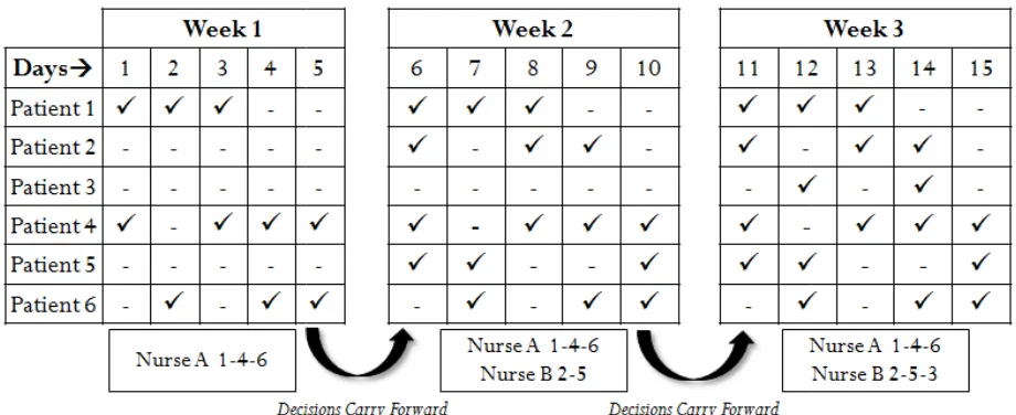
Figures 4 and 5 below illustrate the difference between the week by week and the

long-term template planning strategies. In this very simple example, we consider a 3 week long

planning horizon and assume that each nurse can visit at most 3 patients in a day. In both

approaches, Patients 1, 4 and 6 need to be seen from weeks 1 through 3, but patients 2, 5 and 3

only enter the home care program in weeks 2 and 3. When planning on a weekly basis, the

nurse-patient assignments from week 1 are carried over to week 2 and only those nurse-patients for a given

week are considered. When building long-term plans however, all patients, including those who

don’t start their home care program until weeks 2 or 3 are considered. While both planning

strategies use the ConRTR templates, they differ in how much information about future patients

they incorporate into the early planning stages. As a result, in week 1, with the WBW strategy,

we need only one nurse to visit all patients. In week 2, however, two new patients make requests

and a second nurse is needed in order to be able to complete all visits. In the long-term plan

however, the nurse-patient assignments are slightly different – Nurse A visits patients 1 and 4,

and nurse B visits patient 6. Because we planned for the patients who need to only be visited in

weeks 2 and 3 ahead of time, we are able to create a schedule with a more balanced workforce

(44)

[image:44.612.90.550.77.265.2] [image:44.612.83.559.312.489.2]

Figure

5.2. Experimental design

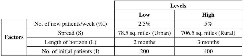
Our experimental design consists of 16 randomly generated instances spanning four factors with

two levels each. The four factors are the number of new patients added per week, the density of

population (i.e. rural or urban), the length of the planning horizon and the number

patients. We used a full factorial design; the levels for each factor are given in Figure Figure 4 - Week by Week Planning

Figure 5 - Long-term Template Planning

esign consists of 16 randomly generated instances spanning four factors with

population (i.e. rural or urban), the length of the planning horizon and the number

patients. We used a full factorial design; the levels for each factor are given in Figure

esign consists of 16 randomly generated instances spanning four factors with

population (i.e. rural or urban), the length of the planning horizon and the number of initial

(45)

Levels

Low High

Factors

No. of new patients/week (%I) 2.5% 5%

Spread (S) 78.5 sq. miles (Urban) 706.5 sq. miles (Rural)

Length of horizon (L) 2 months 3 months

[image:45.612.100.513.71.167.2]

No. of initial patients (I) 200 400

Figure 6 - Factors and Levels for Experimental Design

We next describe some assumptions regarding the instances. First, we assume that each

period is a five-day week. Therefore, a two-month horizon consists of 40 days, or 8 five-day

weeks, and a three-month horizon consists of 60 days or 12 five-day weeks. Second, each patient

has a 70% chance of being seen on each day of the week. In the rare event that no days are

selected for a patient, we assume that the patient doesn’t need to be visited. Once a visit

frequency and schedule is determined, it does not change for the rest of the patient’s episode of

care. Third, we consider a circular region with a radius of 5 miles for urban settings and 15

miles for rural settings. We do so because we assume that the most a nurse will travel in an urban

setting is 10 minutes; at a speed of 60 miles per hour, that translates to a distance of 10 miles or 1

mile per minute. Similarly, in a rural setting, we assume that a nurse will travel at most 30

minutes to visit a patient, or equivalently, at a speed of 60 miles per hour, 30 miles. Therefore,

urban instances are spread over a 5 mile radius with an area of 78.5 sq. miles and rural settings

are spread over a 15 mile radius and an area of 706.5 square miles. Fourth, each nurse may work

at most ten hours a day. Fifth, travel time between two patients is determined by the geographical

distance, d, calculated by the Haversine formula as given below, where lat is the latitude in

radians, lon is the longitude in radians and R is the radius of the earth

a=sin²(Δlat/2)+cos(lat1)*cos(lat2)*sin²(Δlong/2)

(46)

Sixth, for our experiments we consider only a single depot where nurses start and end their day at

the agency. Seventh, for our initial analysis, based on our interviews with the home care agency,

we assume that each patient needs to be visited for an hour. However, we also discuss our

subsequent experimentation studying instances with 30-minute visit durations. Finally, while our

initial experimental design considers a growing demand scenario where new patients only enter

the home care program, later experiments consider the possibility of patients also leaving the

program as their care period ends as in a period of steady demand.

We use the following performance measures in our analysis:

1. Total Travel Time: Travel time is the total time spent by each nurse, N, in traveling to each

patient in the set P, as required, and measured across all days, D in the planning horizon.

Total travel time = ∑ ∑ 16/)Q )Q /7)RQ / S7 T7*

2. Average Value Added Utilization: Value-added (VA) utilization represents the amount of

time nurses spend providing care. It is determined by the average amount of time nurses

spend with their patients over the average total time they work by week.

Avg. VA Utilization per week = ∑ UVWXY Z[[\X] ^_V V`[ a[b cb_[

∑ UVWX Y Z[[\X] bcV[ X[dVe a[b cb_[

3. Dispersion in Number of Nurses: The dispersion is measured by the standard deviation in

the number of nurses working on a weekly basis. In addition, we also report the average

number of nurses scheduled across the horizon, and the maximum number of nurses

scheduled at any week during the planning horizon. These metrics will help establish the

staffing requirements for a given planning horizon.

4. Average number of patients: This metric is used to determine the number of patients, on

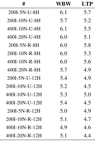
average, seen by each nurse on a daily basis over the horizon. A higher value is desirable

because it indicates that within a given restriction on the maximum number of hours a nurse