http://dx.doi.org/10.1080/19401493.2015.1110621
Characterization of an airflow network model by sensitivity analysis: parameter screening,
fixing, prioritizing and mapping
F. Monari∗and P. Strachan
ESRU, University of Strathclyde, 75 Montrose Street, Glasgow G1 1XJ, UK (Received 19 June 2015; accepted 16 October 2015)
Due to the over-parameterized models in detailed thermal simulation programs, modellers undertaking validation or cal-ibration studies, where the model output is compared against field measurements, face difficulties in determining those parameters which are primarily responsible for observed differences. Where sensitivity studies are undertaken, the Morris method is commonly applied to identify the most influential parameters. They are often accompanied by uncertainty analysis using Monte Carlo simulations to generate confidence bounds around the predictions. This paper sets out a more rigorous approach to sensitivity analysis (SA) based on a global SA method with three stages: factor screening, factor prioritizing and fixing, and factor mapping. The method is applied to a detailed empirical validation data set obtained within IEA ECB Annex 58, with the focus of the study on the airflow network, a simulation program sub-model which is subject to large uncertainties in its inputs.
Keywords: global sensitivity analysis; airflow networks; calibration
1. Introduction
Current detailed building energy simulation (BES) tools are capable of representing the main phenomena determin-ing the thermal and energy performance of builddetermin-ings. How-ever, this achievement in terms of accuracy and fidelity in representing reality entails a high level of complexity of building energy models. In particular, BES models have complicated structures consisting of many in-built sub-models that attempt to represent the physical reality and large numbers of input parameters. Modellers undertaking validation studies find it difficult to identify which param-eters are responsible for observed differences between measurements and predictions; those undertaking calibra-tion studies find it difficult to determine which parameters should be adjusted to improve the correspondence between measurements and predictions. Additionally, all the mod-elling process is affected by uncertainties which, because of the interactions linking the various model inputs, unpre-dictably propagate through the computer code, resulting in uncertainty in the model predictions.
To build accurate models and to reduce these mod-elling uncertainties, it is necessary to utilize a detailed building specification. In practice, many model inputs are often not available. Thus although BES tools can be used to predict the detailed spatial and temporal variations in energy and indoor environmental performance, it is dif-ficult to judge the predictive accuracy because of these modelling uncertainties. Ideally, model output uncertainty
*Corresponding author. Email:fi[email protected]
would routinely be quantified to allow the robustness and reliability of model predictions to be assessed. However in practice, this is seldom the case because of the lack of support to allow users to take into account uncertain-ties in predictions. The only attempt known to the authors to embed uncertainty analysis (UA) in BES programs is by Macdonald and Strachan (2001) based on the dynamic simulation tool ESP-r (Clarke2001).
There have been recent attempts to develop methods to tackle these issues and at the same time to better understand and characterize modelling uncertainty propagation within BES tools. In particular, sensitivity analysis (SA) has been increasingly applied in a stand-alone fashion or as a step in more structured procedures, in order to investigate how model parameter uncertainties influence model behaviour and to address the following issues:
• identifying the most influential variables,
• quantifying output uncertainty,
• understanding the relations between inputs, and inputs and outputs,
• supporting decision-making,
• solving identifiability problems.
An extensive review of SA techniques applied to BES can be found in Tian (2013), while a more general treatment focusing on the different problems that different SA meth-ods can solve is in Saltelli et al. (2002).
© 2016 The Author(s). Published by Taylor & Francis.
SA is usually applied by itself to quantify the uncer-tainty in the model output produced by uncertainties in the model parameters and to understand which are the most influential inputs or, more generally, what the relationships are between the model parameters and model outputs. In Corrado and Mechri (2009), the authors apply the Morris method (1991) and Monte Carlo simulation to identify the most influential factors and the overall output uncertainty for a monthly quasi-steady simplified regulatory model describing a residential building in Turin, Italy. A simi-lar approach is adopted in Garcia Sanchez et al. (2014) to investigate a dynamic ESP-r model representing an apart-ment building in Spain. In this study, the Morris method in its extended version (Campolongo and Braddock1999) is used to evaluate the first- and second-order effects of the several model parameters. The authors, also, outline a framework to classify effect typologies.
In Spitz et al. (2012), a three-step SA is performed on a detailed EnergyPlus model of the INCAS (Instrumenta-tion of new solar architecture construc(Instrumenta-tions) experimental platform of the French National Institute of Solar Energy (INES) in Le-Bourget-du-Lac, France. The objectives are to determine influential parameters, to identify the influ-ence of parameter uncertainty on the building performance and quantify the model output uncertainty. The first two steps of the procedure consist of applying local sensitiv-ity and correlation analysis in order to single out the most important factors (MIF) and then to group model inputs. Finally, global sensitivity analysis (GSA) is undertaken to quantify model output uncertainty and apportion it among the selected most influential parameters.
In Eisenhower et al. (2012), the authors analyse a complex building model having a large number of model parameters (1000) through variance, L1 norm- and L2 norm-based sensitivity measures. Also a method to break down the sensitivity of the model according to its many part and sub-models is explained. In order to speed up the calculations, a meta-model based on support vector regression is used to approximate the detailed BES.
Hopfe and Hensen (2011), Bucking, Zmeureanu, and Athienitis (2013), Rysanek and Choudhary (2013) and Booth and Choudhary (2013) are examples wherein SA is used to support decision-making at different levels. In Hopfe and Hensen (2011), Bucking, Zmeureanu, and Athienitis (2013) and Rysanek and Choudhary (2013), dif-ferent sensitivity and uncertainty analysis approaches are applied to drive the building design and retrofit accord-ing to different objectives. Booth and Choudhary (2013) present a methodology combining, parameter screening with the Morris method, calibration and probabilistic SA of housing stock models based on normative calculation methods to aid decision-making.
In several studies, SA is used to aid model valida-tion or calibravalida-tion. In these problems, SA can be used to reduce model dimensionality through parameter screen-ing, and calculate prediction uncertainties in order to better
compare simulation outcomes with target measurements. In Aude, Tabary, and Depecker (2000), a validation method for BES codes is proposed, which aims to improve the common practice of comparison between simulation out-puts and experimental results by also taking into account the uncertainties in the former. In particular, uncertain-ties in the numerical results are determined through an SA carried out by an adjoint-code method. In Heo, Choud-hary, and Augenbroe (2012) and Heo, Augenbroe, and Choudhary (2013), the Morris method is employed to iden-tify the most influential variables, on which to focus the subsequent calibration procedures for assessing the imple-mentation of energy conservation measures, with simpli-fied regulatory models on office buildings in Cambridge, United Kingdom. The same SA technique is adopted in Kim et al. (2014) to reduce the dimensionality of an Ener-gyPlus model of an office building in South Korea, in the context of a comparison study between stochastic and deterministic calibration methods.
Besides parameter screening, in Reddy, Maor, and Pan-japornpon (2007a,2007b), Cipriano et al. (2015) and Sun and Reddy (2006), different SA methods are used to solve identifiability problems. In Reddy, Maor, and Panjaporn-pon (2007a,2007b) and Cipriano et al. (2015) similar cali-bration procedures are described employing regional SA to select the model parameters that can be identified through iterative Monte Carlo filtering. Statistical tests are used to compare empirical density distributions of parameter samples giving acceptable and unacceptable model realiza-tions, depending on the values of Coefficient of Variation of the Root Mean Squared Error and the Normalized Mean Bias Error, in order to assess the statistical significance of each factor in improving the goodness of the fit with the target data. In Sun and Reddy (2006), an extension to the methodology depicted in Reddy, Maor, and Panjapornpon (2007a,2007b) is presented. The authors propose the use of approximations of the partial derivatives and Hessian matrix of the adopted objective function, to identify model parameters to which model calibration is most sensitive and that are least correlated with other inputs.
can lead to the selection of too few parameters, thereby excessively reducing the degrees of freedom of the model. The main consequence is to work with over-simplified models which poorly represent the original model. It is believed that the use of quantitative techniques to com-plement the qualitative screening methods would help to identify the most important model inputs for further analysis.
This study proposes an approach to SA of BES employ-ing qualitative and quantitative methods in order to aid calibration and validation studies. The main objectives are to measure the extent of the simplifications induced by considering only qualitative sensitivity results and to gain information in order to reduce prior parameter uncertain-ties, thus facilitating parameter identification. Quantita-tive methods cannot be applied directly considering every model input due to the prohibitive computational load. Thus qualitative screening is performed to reduce model dimensionality and group parameters, and its efficacy is assessed by quantifying to what extent the resulting model is representative of the original. The additional simulations required are used to acquire knowledge aiding calibration or validation.
The Morris method and the Sobol method have been employed because they are GSA techniques and model independent. It is believed that these two properties are indispensable for an SA methodology that can be applied to BES. Unlike local SA methods, which change one fac-tor at a time with respect to a default configuration, and thus are unable to capture higher order interactions, GSA methods measure the sensitivity of a model by varying all their inputs at the same time, and therefore they are able to give an adequate picture of first as well as higher order effects. Model independence is the capability of a sensitiv-ity technique to perform well regardless the mathematical structure of the model, so as to correctly characterize its sensitivity irrespective of whether it is additive, linear or non-linear.
The proposed procedure is applied to a particular sub-model in order to illustrate the use of SA to study a modelling domain where there are large uncertainties in modelling assumptions and model parameters. The cho-sen focus is an airflow network model reprecho-senting ven-tilation and infiltration in an experimental facility used for calibration and validation exercises in the context of the IEA (International Energy Agency) EBC (Energy Building and Communities) Annex 58 (IEA EBC Annex 582011–2015). Among several specific phenomena such as air stratification and convective heat transfer which con-tribute to the overall model uncertainty and behaviour, a previous calibration study (Strachan et al.2015a) on one of the buildings in the experimental facility showed that accurate modelling of ventilation and infiltration had a sig-nificant impact in improving predictions compared to a simplified approach using average constant flow rates to represent infiltration.
During the analysis the main sensitivity model char-acteristics are investigated. The most influential and least influential factors are identified and their effects quanti-fied in order to assess if a model considering only the former is a good approximation of the original. Subse-quently the model inputs are mapped according to their influence in producing model outputs close to the target measurements.
Some novel methods to perform UA and calculation of sensitivity indexes are also investigated in this paper. The SA is preceded by a UA which has the purpose of deter-mining prior uncertainties for the model factors. This is not an easy task because of the difficulty in determining prior uncertainties of some of the input parameters, and because of the impact associated with the selection of these prior uncertainties on the SA. Also vectorial model inputs (sometimes referred to as multidimensional input param-eters), for example, weather factors, are rarely considered in SA and their uncertainties are usually assumed constant over time. Such an approach neglects the time-varying conditions affecting the measurements of these entities, which may have different levels of uncertainty during the monitoring period. In order to account for this aspect and be as rigorous as possible, bootstrapping and smoothing techniques are employed to investigate how uncertainty magnitudes may vary during the experiment.
BES produce time series as outputs and in most approaches the calculation of SA indexes is carried out for each time step or by considering integrals of output vari-ables and distances from reference values. In the former case, while it is possible to see how the model sensi-tivity changes over time a large and redundant amount of information is produced which is hard to analyse and summarize. The latter approach produces more concise results but at the same time does not consider the dynam-ics of the model outputs in an adequate way. To achieve concise information about model sensitivity considering output dynamics, new approaches based on principal com-ponent analysis (PCA) are employed and an expansion of the Morris method is proposed.
The first part of the paper describes the experiment and the model used as the example application. This is fol-lowed by details of the UA performed in order to assess prior parameter uncertainties, and then a description of the sensitivity methods used. Finally, the main results are dis-cussed and the conclusions drawn regarding the efficacy of the methods investigated.
2. Experiment
In this section, the experiment is described with particular focus on the information important for the flow network modelling.
validation exercise undertaken as part of the IEA EBC Annex 58 work programme. The experiment was per-formed by the Fraunhofer Institute in Holzkirchen, Ger-many, during April and May 2014, in a flat and unshaded area. For a detailed description the reader is referred to Strachan et al. (2015b).
Figure1shows the layout of the ground floor wherein the experiment was performed. The attic and basement of the building were considered as boundary spaces, with the internal air temperatures kept constant at 22◦C. The doors connecting the living room to kitchen, lobby and bedroom 2 were sealed, while ventilation was allowed between the living room, corridor, bathroom and bed-room 1. Blinds were kept closed in the kitchen, lobby and bedroom 2 (NORTH_ZONE) and attic, but were kept open in the living room, corridor, bathroom and bedroom 1 (SOUTH_ZONE). Air leakage was experimentally inves-tigated by performing pressurization tests at the standard pressure difference of 50 Pa.
The experimental schedule was the following:
• Days 1–10: initialization at constant temperature of 30◦C in SOUTH_ZONE, bedroom 1 and bathroom, and 22◦C in attic, cellar and NORTH_ZONE.
• Days 11–24: Randomly Ordered Logarithmically distributed Binary Sequence (ROLBS) of heat pulses in SOUTH_ZONE and constant temperature of 22◦C in attic, cellar and NORTH_ZONE.
• Days 25–31: constant temperature of 30◦C in SOUTH_ZONE and 22◦C in attic, cellar and NORTH_ZONE.
• Days 32–40: Freefloat in SOUTH_ZONE, and 22◦C in attic, cellar and NORTH_ZONE.
This study focuses on the ROLBS phase, in which pseudo-random heat pulses (van Dijk and Tellez 1995) are injected in the SOUTH_ZONE; this is done so that these heat inputs are not correlated with the solar heat inputs. The heating system was composed of lightweight electric heaters with fast response having a split coeffi-cient between convective and radiative heat gains (C/R) of 70%/30% according to the manufacturers. The distribution of these devices is shown in Figure1.
Mechanical ventilation was used during the entire experiment to avoid excessive overheating. The ventilation inlet was in the living room and there were two extrac-tion points in the bathroom and in bedroom 1. The inflow rate was set to 60 m3/h and the outflow rates were set to 30 m3/h for both extraction points. The ventilation system had ducts going from the basement to the living room and from the living room to the attic.
The provided data set was comprehensive, consist-ing of 50 variables measured with one-minute time steps. Those employed in the analysis are external tempera-ture, wind speed and direction, internal zone temperatures, zone sensible heat loads, supplied air temperature, base-ment air temperature, attic air temperature and the ROLBS sequence of heat injections.
3. Model
[image:4.610.124.486.445.725.2]A detailed ESP-r model was created from the provided experimental specification and on choices and assumptions
according to best practice and modeller experience. The building geometry was completely respected as well as the compositions of the construction elements and exper-imental schedule. The boundary conditions as determined by the external weather were imposed on the model. The resulting BES model was made of seven thermal zones reflecting the different rooms. Since the study focuses on the airflow network sub-model, only the parameters affect-ing the airflow have been considered. In particular, material properties have been fixed to the values prescribed by the specifications. A diagram of the airflow network model is shown in Figure2.
Crack components were used to represent connec-tions between the internal and external environments and between SOUTH_ZONE and NORTH_ZONE. Constant flow rate components were adopted to model the mechan-ical ventilation system at the supply and extraction points. Bi-directional flow components were employed for the links between the living room, corridor, bathroom and bed-room 1. The resistances of these large openings are very small compared to the other openings, so parameter uncer-tainties associated with them have been deemed negligible and were neglected in the analysis. For more details regard-ing the mathematical modellregard-ing of the components used
to build the flow network model, the reader is referred to Hensen (1991).
4. Uncertainty analysis
As mentioned in Section 1, one feature of this study is the consideration of vectorial (or multidimensional) inputs as well as scalar (or unidimensional) ones.
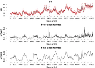
The former consists of variables described by time series and therefore their values change during the exper-iment and simulations. To adequately characterize the uncertainties for such factors it is necessary to define multidimensional probability distributions depicting time-varying marginal probability distributions and correla-tion patterns relative to observacorrela-tions at different time steps. Indeed, especially for weather factors such as wind speed (Figure 3), monitoring conditions as well as unob-served phenomena influencing the measurements may result in time-varying magnitudes of the measurement random errors.
The multidimensional parameters considered are the following:
[image:5.610.110.499.370.717.2]• Wind speed, wind direction and external air tem-perature: these factors are responsible for the main
Figure 3. Wind speed – smoothing model fit (red dots: observations, black line: model fit), prior uncertainty from Bootstrap and final uncertainties from smoothing.
boundary conditions imposed by the exterior envi-ronment on the building that affect the airflow. In particular, they determine the pressures at the bound-ary nodes of the flow network.
• Temperature set-points for the north zones, base-ment and attic: non-perfect control and systematic and random variability of these variables produce changes in the relative zone pressures thus affecting the ventilation regime.
• ROLBS heat impulses for the south zones: as the main experimental heat inputs, it is expected that these variables have a major influence on the con-ditions determining ventilation.
To suitably represent the uncertainties of unidimen-sional model parameters that do not change during the experiment and simulations, it is sufficient to define uni-variate probability distributions. The parameters of this kind considered are the following:
• Crack dimensions: because of the relatively low infiltration rates, only small cracks have been assumed as connections between the interior and the exterior environments. Their dimensions are sources of uncertainties since they are difficult to measure.
• Wind-induced pressure coefficients: these parame-ters, together with wind speed, wind direction and ambient air temperature, determine the pressures at the boundary nodes. As they have not been directly observed, they are subject to major uncertainties
and one objective of this study is to assess their influence.
• Mechanical ventilation flow rates: particular atten-tion was paid in setting up the experiment to ensure a balance between inflow and outflow from the mechanical ventilation; nevertheless there is the pos-sibility of imbalances due to systematic and random measuring errors which could have a relevant influ-ence on the ventilation regime, so these uncertainties were included in the analysis.
• Ratios between convective and radiative heat gains from ROLBS sequences (C/R): besides possible inaccuracies in these ratios, their values could change because of the particular experimental condi-tions, zone air temperatures and velocities. For these reasons, they would be better represented by multi-dimensional probability distributions. However the model allows only constantC/R splits, and thus it was necessary to approximate them with univari-ate probability density distributions. Variations in these parameters may influence the airflow. In par-ticular, the ratios of convective and radiative gains should determine quicker or slower changes in the zone pressures.
4.1. Multidimensional variables
The measurements are inevitably affected by errors. Two kind of uncertainties are taken into account: systematic and random. The former are intrinsic properties of the sen-sors used in the monitoring. They can be assumed constant during time or as functions of the measured values and producing always the same bias in the data meaning that a certain sensor always overestimates or underestimates the “true value”. The latter kind of errors is unpredictable and is produced by the stochastic character of the moni-tored process or by the effects of unobserved phenomena on the measurements. Generally, and in this study, they are assumed to be normally, independently and identically distributed variables.
Under such assumptions, the model assumed for a cer-tain measured variable (ηηη) including error terms is the following:
ηηη= ¯ηηη+s+r, (1)
whereηηη¯ is the “true value”,srepresents systematic errors andrindicates random errors.
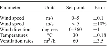
The properties ofswould allow the data to be corrected if the exact magnitude and direction of the errors were known. The provided information specified only maximum bounds for such entities and did not allow an accurate eval-uation, although all sensors were calibrated as expected in a high-quality experiment. Therefore, their magnitudes and directions were treated as random variables by defin-ing normal distributions with zero mean and standard deviations half the sensor errors estimated during sensor calibration (Table1). The uncertainties related to system-atic errors were simulated by drawing values from these distributions and adding them to the corresponding time series.
[image:7.610.86.273.650.731.2]The estimation of random errors is usually done through smoothing methods (Craven and Wahba 1978; Hutchinson and de Hoog1985; Johnstone and Silverman 1997) and should be based on a priori information about the possible error model, thus avoiding to generate spuri-ous data by excessive smoothing. Establishing a prior error model is not an easy task as the modelled entity is hid-den in the data and unpredictable. Useful information about the local precision of the measurements can be gained by evaluating their local variance. In this case, data sampled at high frequency were available, thus it was decided to use Bootstrap (Efron and Tibshirani1993) to calculate the
Table 1. Systematic sensor errors.
Parameter Units Set point Error
Wind speed m/s 0–5 ±0.1
Wind speed m/s >5 ±10%
Wind direction degrees 0–360 ±1
Temperatures ◦C 30 ±0.18
Ventilation rates m3/h 60 ±3.5
10-minute averages from the raw 1-minute time series and to estimate the standard errors relative to these estimates. In this way, it was possible to reduce the simulation bur-den while keeping an adequate simulation time step and to infer a reasonable prior probability density distribution for the uncertainties () affecting the averaged time series (x):
x = ˆx+, (2)
∼N(0,−1), (3)
−1 =diag(σ2
i, i=1,. . .,n), (4)
where diag(·)represents an operator that creates a diagonal matrix with elements comprising the given arguments,σiis the estimated standard error relative to theith average,xˆis the unknown mean vector andnis the length ofx.
Then, smoothing with roughness penalty (Ramsay and Silverman 2005) was applied to x, with the purposes of inferring xˆ, refining the prior error model considered, investigating correlation patterns and providing for miss-ing values in the data. In this framework, measurements are represented through a suitable basis expansion:
x= Q
q=1
kq(t)wq+=K w+, (5)
wherekq(t)are the chosen basis functions,wqare the cor-responding coefficients andtis the observation time vector. In this study, B-splines were used as basis functions. It is important to notice that in Equation (5), the unknown vectorxˆ has been represented with the function:
ˆ
x = ˆx(t)= Q
q=1
kq(t)wq.
The smoothing is performed by estimating w accord-ing to a regularized least-square criterion, penalizaccord-ing the “roughness” of the data:
(ˆx−K w)T(xˆ−K w)+λwTRw, (6)
where λ is a parameter controlling the power of the smoothing and R is the matrix quantifying the “rough-ness”. In this case, it was decided to represent this entity with the curvature ofx(ˆ t), that is, the square of its second time derivative. This measure of roughness is suggested in Ramsay and Silverman (2005) and is based on the ratio-nale that an infinitely smooth function, like a straight line, has its second derivative always equal to zero, while a highly variable function will show, at least over some ranges, large values for its second derivative. Therefore, Ris defined as:
R=
D2KD2KTdt,
estimates for such variables are given by
ˆ w=Sx,
whereS=(λR+KTK)−1KT.
Thus, in the smoothing, the standard errors calculated through Bootstrap act mostly as weights relative to the accuracies of the values inxˆ, so that the smoothing model tries to obtain a closer fit forxiwith lowσi. An example of the uncertainties estimated with the above-explained two-step procedure is provided in Figure3, for the wind speed. The measurements of this variable were showing high local variability and the uncertainties calculated through Bootstrap appear to overestimate the extent of possible ran-dom errors, showing values eight times higher than the respective systematic errors. Refining the error model by smoothing provided values more in agreement with the high monitoring standards characterizing the experiment.
ˆ
w depends on the smoothing parameter λ since the matrixSis a function of it. For values ofλclose to zero, the model in Equation (5) tries to fit exactly the obser-vations even if this causes over-fitting. For values of λ approaching ∞, the model will perform a standard lin-ear regression which can be poorly representative of the main dynamical trends. Thus this parameter is particularly important and must be chosen carefully. Ramsay and Sil-verman (2005) suggest that it is determined in order to minimize the generalized cross validation criterion (GCV):
n−1SSE
(N−1tr(I−S))2 =
N N−df(λ)
SSE
N−df(λ), (7)
where tr(·)indicates the trace operator, df(λ)=tr(S)are the degrees of freedom of the smoothing model and SSE is the sum of squared residuals. GCV can be seen as a discounted mean-squared error measure according to the degree of freedom as a function of λ. The same approach was adopted in this work and the software pack-age described in Ramsay, Hooker, and Graves (2009) was used to carry out the necessary calculations.
Because of the assumption of the noise being Gaus-sian (Equation (3)), wˆ will be normally distributed with mean wˆ and covariance matrix S−1ST. Hence for the property of Gaussian distributions, the following has been assumed for multidimensional variable x (Ramsay and Silverman2005):
x∼N(Kwˆ,K S−1STKT). (8)
The probability density distributions defined by Equation (8) were used to draw random samples for the multidimensional variables. The systematic error terms were then added.
4.2. Unidimensional variables
Most of the univariate variables considered have not been directly observed during the experiment. Thus it
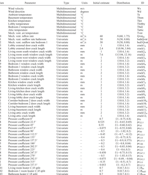
was necessary to estimate their uncertainties from indi-rect measurements, analyst experience and information from literature review. The defined probability distribu-tions describing these parameters are listed in Table2.
4.2.1. Ventilation flow rate
Ventilation flow rates for mechanically supplied and extracted air were measured during the experiment with one-minute time step. However, the flow network model represents mechanical ventilation inflow and outflow with constant volume flow rate components (Hensen 1991), and it does not allow the use of time-varying flow rates. Therefore, univariate probability distributions were used to summarize the information relating to such variables. A model similar to the one adopted for multidimensional variables was considered:
˙
V= ˆ˙V+s+, (9)
where V˙ and Vˆ˙ indicate a certain volume flow rate and its estimate, sis the systematic error term and depicts the random uncertainty.Vˆ˙ and were assessed by boot-strapping the entire time series and s was defined in a similar way as for multidimensional variables, as equal to half the sensor error provided with the experimental spec-ifications (Table1). The resulting probabilistic model for
˙ Vis
˙
V∼N(Vˆ˙,σ2), (10)
σ2=s 2
2
+σ2
, (11)
where σ2
is the variance of the independently and
identically distributed variable.
Assuming the variance of V˙ as indicated in Equation (11) is a simplification, since random errors will not always be in the same direction as systematic errors. However, estimatingV˙from the entire time series produces random uncertainties negligible compared to the system-atic ones. In particular, σ has estimates of 0.0032 and 0.0035 m3/h for inflow and outflow, respectively, whiles is equal to 3.5 m3/h. Thus even if it results in a slight overestimation of the uncertainties, the assumption in Equation (11) can be considered reasonable.
4.2.2. Crack lengths and widths
The length and width of the crack components have been evaluated according to the results given by the pressuriza-tion test results at 50 Pa. Two blower door tests were per-formed, one for the whole ground floor and one involving only the SOUTH_ZONE:
• whole ground floor: 1.54 ac/h.
Table 2. Considered parameters and relative prior distributions.
Num Parameter Type Units Initial estimate Distribution ID
1 Wind velocity Multidimensional m/s Ws
2 Wind direction Multidimensional degrees Wd
3 Ambient temperature Multidimensional ◦C Te
4 Basement temperature Multidimensional ◦C Tbsm
5 Kitchen temperature Multidimensional ◦C Tkit
6 Lobby temperature Multidimensional ◦C Tlobby
7 Bedroom 2 temperature Multidimensional ◦C Tbd2
8 Attic temperature Multidimensional ◦C Tattic
9 Mech. vent. air temperature Multidimensional ◦C Tvnt
10 Mech. vent. inflow rate Univariate m3/s 60 N(60, 1.75) Qvntliv
11 Mech. vent. outflow rate bathroom Univariate m3/s 30 N(30, 0.88) bathQvnt
12 Mech. vent. outflow rate bedroom 1 Univariate m3/s 30 N(30, 0.88) bed1Qvnt
13 Lobby external door crack width Univariate mm 1 U(0.4, 1.6) crack1w
14 Lobby external door crack length Univariate m 2.4 U(0.96, 3.84) crack1l
15 Living room south window crack width Univariate mm 1 U(0.4, 1.6) crack2w
16 Living room south window crack length Univariate m 7.6 U(3.04, 12.16) crack2l
17 Living room west window crack width Univariate mm 1 U(0.4, 1.6) crack3w
18 Living room west window crack length Univariate m 2 U(0.8, 3.2) crack3l
19 Bedroom 1 window crack width Univariate mm 1 U(0.4, 1.6) crack4w
20 Bedroom 1 window crack length Univariate m 2 U(0.8, 3.2) crack4l
21 Bathroom window crack width Univariate mm 1 U(0.4, 1.6) crack5w
22 Bathroom window crack length Univariate m 2 U(0.8, 3.2) crack5l
23 Bedroom 2 window crack width Univariate mm 1 U(0.4, 1.6) crack6w
24 Bedroom 2 window crack length Univariate m 2 U(0.8, 3.2) crack6l
25 Kitchen window crack width Univariate mm 1 U(0.4, 1.6) crack7w
26 Kitchen window crack length Univariate m 2 U(0.8, 3.2) crack7l
27 Living-kitchen door crack width Univariate mm 2 U(0.8, 3.2) crack8w
28 Living-kitchen door crack length Univariate m 1 U(0.4, 1.6) crack8l
29 Living-lobby door crack width Univariate mm 2 U(0.8, 3.2) crack9w
30 Living-lobby door crack length Univariate m 1 U(0.4, 1.6) crack9l
31 Corridor-bedroom 2 door crack width Univariate mm 2 U(0.8, 3.2) crack10w
32 Corridor-bedroom 2 door crack length Univariate m 1 U(0.4, 1.6) crack10l
33 Living-basement crack width Univariate mm 2 U(0.8, 3.2) crack11w
34 Living-basement crack length Univariate m 1 U(0.4, 1.6) crack11l
35 Living-attic crack width Univariate mm 2 U(0.8, 3.2) crack12w
36 Living-attic crack length Univariate m 1 U(0.4, 1.6) crack12l
37 Pressure coefficient 0◦ Univariate – 0.7 U(−0.75, 0.8) pc0
38 Pressure coefficient 22.5◦ Univariate – 0.525 U(−0.65, 0.69) pc22.5
39 Pressure coefficient 45◦ Univariate – 0.35 U(−0.60, 0.42) pc45
40 Pressure coefficient 67.5◦ Univariate – −0.075 U(−0.55, 0.04) pc67.5
41 Pressure coefficient 90◦ Univariate – −0.5 U(−1.02, 0.2) pc90
42 Pressure coefficient 112.5◦ Univariate – −0.45 U(−0.7,−0.12) pc122.5
43 Pressure coefficient 135◦ Univariate – −0.4 U(−0.75, 0.5) pc135
44 Pressure coefficient 157.5◦ Univariate – −0.3 U(−0.9, 0.375) pc157.5
45 Pressure coefficient 180◦ Univariate – −0.2 U(−0.8, 0.04) pc180
46 Pressure coefficient 202.5◦ Univariate – −0.3 U(−0.85, 0.04) pc202.5
47 Pressure coefficient 225◦ Univariate – −0.4 U(−0.6, 0.3) pc225
48 Pressure coefficient 247.5◦ Univariate – −0.450 U(−0.75, 0.15) pc247.5
49 Pressure coefficient 270◦ Univariate – −0.5 U(−1.03, 0.15) pc270
50 Pressure coefficient 292.5◦ Univariate – −0.075 U(−0.49,−0.04) pc292.5
51 Pressure coefficient 315◦ Univariate – −0.35 U(−0.51, 0.7) pc315
52 Pressure coefficient 337.5◦ Univariate – −0.053 U(−0.2, 0.7) pc337.5
101 Living room heaterC/Rsplit Univariate – 0.7 N(0.7, 0.1) C/Rliv
102 Bedroom 1 room heaterC/Rsplit Univariate – 0.7 N(0.7, 0.1) C/Rbed1
103 Bathroom heaterC/Rsplit Univariate – 0.7 N(0.7, 0.1) C/Rbath
The former should give a good picture of the total ground floor infiltration, while the latter represents a mix between infiltration and ventilation between north and south zones. For the two tests, the total leakage area (A) was derived according to the “orifice equation” (Hensen1991):
˙ m=CdA
2ρP, (12)
where m˙ is the mass flow rate, Cd =0.61 is the dis-charge coefficient, ρ=1.2 kg/m3 is the air density and
P=50 Pa is the pressure difference. From the result for the whole ground floor,A has been decomposed rel-ative to NORTH_ZONE and SOUTH_ZONE according to volume proportions. Then from the result regarding only SOUTH_ZONE, it was possible to assess the leak-age area responsible for ventilation only, by difference. Crack lengths were estimated depending on opening char-acteristics and experience and consequently the widths were calculated. Uniform distributions involving ranges of ±60% of the estimated values were adopted for these variables.
4.2.3. Wind-induced pressure coefficients
Wind-induced pressure coefficients are possibly the most uncertain variables in the model. No information about their uncertainties came from the experiment and thus suit-able probability distributions have been inferred depending upon data from literature review. A complete treatment of their variability would consider the correlation between them, due to their dependence on wind speed, wind direc-tion, location on the surface and configuration of the sur-rounding area. However, with the available data it was not possible to adequately model such correlation relationships and they have been considered independent. Neglecting the correlation between these model inputs causes overestima-tion of their uncertainties, whereas considering their inter-dependence without any specific measurements may lead to the opposite problem. The former option was selected because it was more conservative.
An extensive review of secondary sources of data for pressure coefficients can be found in Costola, Blocken, and Hensen (2009). This study compares pressure coefficient values from different databases depending on different sheltering conditions and derives plausible variation ranges depending on wind directions relative to surface normals. Such information was integrated with the data available from the ESP-r database, including different aspect ratios for walls, in order to define suitable variation ranges. In the flow network model, each boundary nodes is defined by 16 pressure coefficients for wind directions defined every 22.5◦ relative to the surface normals. The bound-ary nodes considered are those named NORTH, EAST, SOUTH and WEST in Figure2 for a total of 64 pressure coefficients.
4.2.4. Convective/radiative split for heaters (C/R)
In the model only the fractions relating to the convec-tive part were treated as random variables, defining the remaining fractions by difference. An estimate for such variables was given by the heater manufacturer. Therefore, it was considered to be substantially less uncertain than other parameters in the model, and normal probability den-sity distributions with mean 0.7 and standard deviation 0.1 were assumed.
5. Sensitivity analysis
A three-step SA is proposed involving different settings, objectives and methods according to the tasks to perform (Saltelli2002):
• Factor screening (FS): in this setting the Morris method has been applied to the model in order to gain qualitative information about parameter effect magnitudes and understand which variables may have major influences on the model responses.
• Factor prioritizing (FP) and factor fixing (FF): in this setting the Sobol method, a variance-based SA technique, is used to quantify the amount of vari-ance that can be attributed to individual parameters or group of parameters. This allows the identifica-tion of those inputs which should be tuned carefully in order to minimize the model output variance and those inputs which can be fixed to default values because they are responsible for negligible model output variations.
• Factor mapping (FM): in this stage, simulations are weighted according to a chosen criterion and the relative model input vectors are mapped according to their probabilities to produce model realizations close to the target measurements. Furthermore, the importance of the different model parameters that lead to improved calibration is assessed.
FS could be seen as redundant since the same information can be gained from more detailed sensitivity results using FP and FF. However, variance-based methods are particu-larly simulation intensive and because of the large number of parameters involved (103 in the example considered) the number of simulations needed would have been hardly manageable. Thus it has been deemed appropriate to use the Morris method, which has a substantially lower com-putational burden, to gather qualitative information and reduce the dimensionality of the problem by grouping together the parameters having small effects. Then the Sobol method has been used to assess the efficacy of the screening.
sensitivity techniques by following the principles outlined in Campbell, McKay, and Williams (2006) and Lam-boni, Monod, and Makowski (2011). In particular, PCA (Jolliffe2002) is extensively applied to treat vectorial out-puts. Descriptions of the methods used to perform FS, FP, FF and FM with particular emphasis on the modification adopted in order to treat multidimensional outputs follow.
5.1. Factor screening
In this step, the Morris method (Morris1991) is employed to identify the MIF governing the model in order to reduce its dimensionality to a feasible extent for the next phases. In this phase, model inputs are divided into MIF and least important factors (LIF), and eventually grouped.
The adopted technique characterizes the sensitivity of the model to the ith input, through the concept of ele-mentary effects (eei), which can be described as partial derivative approximations:
eei=
f (zi+δδδii)−f(zi)
i
,
wheref (·)represents the model evaluated at a certain input vectorzi,δδδiis a zero vector where only theith position is equal to one andiis the applied variation to theith input. A chosen number r (usually within the range [20, 50]) of elementary effects are calculated according to a facto-rial design, representing the parameter space, defined as described in Campolongo, Cariboni, and Saltelli (2007), which allow the needed information to be obtained with a number of simulations (N) linearly proportional to the number of inputs (n):N =r(n+1).
The empirical absolute means (μ∗i) and the standard deviations (σi) of the derived samples of eei character-ize, respectively, the magnitude and typology of each input effect. In particular, the magnitudes of first-order effects are proportional toμ∗i, while parameters having highσihave significant higher order effects.
To handle the high dimensionality of the ESP-r vecto-rial outputs, it has been necessary to extend the method. For this purpose PCA was used to decompose the gener-ated simulation data set so that each simulation output (y) was represented as follows:
y= Q
q=1
kqwq=K w+, (13)
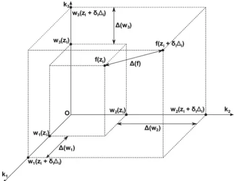
[image:11.610.318.547.69.246.2]where Qis the number of retained orthonormal baseskq andwq are the principal components.Qhas been chosen to explain 99% of the output variance so thatrepresents a negligible amount of the total variability. In this way, the initial data set of dimensionalitym×N, where m is the simulation length, has been reduced toQindependent sets of dimensionalityN×1 suitable to be separately pro-cessed by the Morris method, resulting inQμ∗i,q indexes.
Figure 4. Elementary effect representation in the coordinate system defined by PCA.
In particular each simulation output is represented in the space defined by kq as depicted in Figure4 whereQhas been assumed equal to 3. Thus:
μ∗ i,q=
1
r
r
j=1 (wq,j)
i,j
, (14)
where the meaning of wq,j is indicated in Figure 4,i,j is the variation applied to the ith input in the jth itera-tion of the Morris method. A new sensitivity index, Mi, has been defined and used to perform parameter screening as follows:
Mi= Q
q=1
(μ∗
i,q)2. (15)
Due to the orthonormality properties of kq, the indexMi can be seen as an approximation of the directional deriva-tive in the gradient direction with respect to the ith input in the reference system defined by PCA. In particular, it is a generalization of theμ∗i index for vectorial model out-puts, and it is representative of the first-order effects of each parameter.
The sensitivity indexes employed in the Morris method can be dependent on the variation ranges applied. In partic-ular, leaving the variations applied to each parameter with its own units can produce misleading results since the cal-culated elementary affects will have in turn different units, making it impossible to compare them. To avoid this issue model input samples have been scaled and centred so that each of them has mean equal to zero and standard deviation equal to one.
Due to the qualitative character of the results provided by the Morris method, parameter retention is usually done depending on empirical evaluations. In particular, in this case the 10 factors having the highestMiindexes have been considered sufficient to approximate the original model.
5.2. FP and FF
The purpose of this stage is to extend the qualitative outcomes from the previous analysis by quantifying the amount of model output variance attributable to each model parameter or group of parameters. Through FF the MIF parameters are ranked according to the fraction of model output variance contributed by the parameter. This provides a priority scale for identifying which variables it is necessary to know accurately in order to reduce most of the model output variance. FF provides complementary objectives. In this case, MIF factors are ranked depending on the fraction of model output variance for which they are responsible for including interactions between parameters. This gives information about which factors it is possible to fix to default values because their associated uncertain-ties have negligible influence on model outputs. In this phase, the effectiveness of the previous parameter screen-ing is assessed by calculatscreen-ing the portion of model output variance attributable to the LIF group. The Sobol method (Sobol 2001) has been used to undertake these tasks. It is based on the decomposition of total (or unconditional) model output variance (V(y)) into its conditional compo-nents. By defining with xi the ith model input or set of inputs and withx−iits complement, the variance of a vari-able, y, depending on x can be decomposed as follows (MacFarlan and Graybill1963):
V(y)=V(E(y|xi))+E(V(y|xi)), (16)
V(y)=V(E(y|x−i))+E(V(y|x−i)), (17)
where y|xi andy|x−i indicate the conditionality of vari-ances (V(·)) and estimates (E(·)) on knowingxiandx−i, respectively.
Equations (16) and (17) allow the definition of two sensitivity measures of major importance. In particular, by normalizing these equations by V(y), it is possible to derive the two following indexes as fractions of the total
output variance (Saltelli et al.2002):
Si=
V(E(y|xi))
V(y) , (18)
STi=
E(V(y|x−i))
V(y) , (19)
where Si indicates the portion of V(y) which can be attributed to the first-order effect ofxi and is named
first-order effect. Parameters with high values forSiare respon-sible for most of the output variance, and by knowing their true values it is possible to reduce output uncertainty at least proportionally to the sum of the Si indexes, since higher order effects might actually contribute as well. This can be seen directly from Equation (16). Since V(y)is a constant, factors with high V(E(y|xi))have low expected output variance (E(V(y|xi))).
STirepresents the portion of V(y)left by leaving only xi unknown, that is, the portion of V(y) attributable to all the effects (including first- and high-order effects) of xi and is calledtotal effect. In particular, setting parame-ters with negligible STi to default values should leave a negligible output uncertainty. Similarly ifxihas negligible influence, V(E(y|x−i))will be high since for differentx−i the estimates of the output are sensibly different and thus E(V(Y|x−i))assumes small values.
TheSi index is used in performing FP, while the STi index is employed in carrying out FF. Also, differences in the values of the two indexes indicate howxi act on the model outputs. For similarSi and STi the relative factors have linear and additive effects, while for high STi and lowSi, they exert their influences by interacting with other inputs or through non-linearities. For example, for linear additive models Si=STi and
iSi=1, while for non-linear modelsSi<STi,
iSi<1 and
iSTi>1 since different STimay account for the same higher order effects. The multidimensional integrals involved in the eval-uation of the estimates and variances in Eqeval-uations (18) and (19) are calculated through Monte Carlo estimation. Several estimators have been proposed to perform this task and a comparison study can be found in Saltelli et al. (2010). In this work, the estimator proposed in Saltelli (2002) was chosen.
As in the previous case the sensitivity indexes described above are defined for scalar model outputs. Their calculation can be extended according to Lamboni, Monod, and Makowski (2011) by using PCA to summarize vecto-rial model responses. In particular, letYbe an×mmatrix having as columns the simulation outputs, withYcentred so that each row has mean equal to 0. Then the total vari-ability of the data set represented byYcan be defined as the trace (tr(·)) of its empirical covariance matrix ():
= 1
mYY
T,
It is shown in Lamboni, Monod, and Makowski (2011) that the data set consisting of the sum of the principal compo-nents has the same variance as the original data set, and since it is composed of unidimensional variables, it can be used to replaceyin Equations (18) and (19).
In applying the Sobol method, multidimensional inputs were varied by generating random samples from Equation (8) and then adding the systematic error compo-nent. This approach is not subject to uncertainty overesti-mation.
5.3. Factor mapping
FM is an extension to normal SA which can provide useful information about which parameters it is necessary to focus on in calibration and validation studies. During FS, FP and FF the measures of sensitivity were relative to model output. This may lead to neglecting some variable having a relatively low influence in the model but important for achieving a good fit with the given monitored data. FM, by considering the target measurements as well, provides for this, and integrates the results from the previous phases. It aims to identify input vectors more likely to produce model realizations close to the target observations and thus to determine which model parameters are more powerful in improving the similarity between model predictions and measurements. To perform this task the generalized like-lihood uncertainty estimation (GLUE) framework (Beven and Binley1992) was chosen, in particular the methodol-ogy described in Ratto (2001).
GLUE is a simplified Bayesian method allowing infer-ence about posterior estimates of model parameters and model outputs, which is conditional on the measured data. In the usual Bayesian approach, the joint posterior distribu-tion of the model inputs (x) given the observation set (ζζζ) is defined as
p(x|ζζζ)∝p(ζζζ|x)p(x), (20)
wherep(ζζζ|x)is the likelihood ofζζζ andp(x)is the prior distribution for x. It is then possible to infer the poste-rior estimates and uncertainties for the model inputs and outputs by evaluating the following integrals:
E(y|ζζζ )=y∗=
f (x)p(x|ζζζ)dx, (21)
cov(y|ζζζ )=cov(y∗)
=
(f (x)−y∗)(f (x)−y∗)Tp(x|ζζζ)dx, (22)
E(x|ζζζ )=x∗ =
xp(x|ζζζ )dx, (23)
cov(x|ζζζ )=cov(x∗)=
(x−x∗)(x−x∗)Tp(x|ζζζ)dx, (24)
wheref (·)indicates the computer model. Often the eval-uations of the integrals in Eqeval-uations (21)–(24) are difficult
for detailed computer models requiring the employment of Markov chain Monte Carlo or importance sampling methods and the creation of meta-models to speed up the calculations. Additionally the definition of a proper likelihood equation is not always possible due to lack of information.
The GLUE approach assumes that the model param-eters are generated directly from their prior distributions and an approximate likelihood measure instead of an accu-rate one. In particular, a suitable function depending on the sum of squared residuals (SSE) between model realiza-tions and measured data is assumed as an approximation of a proper likelihood measure. Such function weights more model simulations (and thus the relative input vectors) hav-ing low SSE and vice versa, and it is called “weighthav-ing function” (ω(·)).
The definition ofω(·)is problem dependent and exam-ples can be found in Beven et al. (2000). In this study, it has been defined as follows (Ratto2001):
ω(yi|xi,α)∝
1 2n
n
i=1
(yi−ζζζ )2 −α
, (25)
whereyirepresents theith output dependent onxi, that is, the ith input vector and nis the number of observations.
α can be used to regulate the power of the weighting by concentrating higher values ofω(·)aroundζζζ and is empir-ically chosen in order to achieve a reasonable distribution of the weights over the simulation sample.
It is then possible to weight eachyias follows:
ωi=
ω(yi) m
i=1ω(yi)
. (26)
As Equation (25) is an approximation of a proper likeli-hood measure, ωi are approximations of posterior prob-abilities having drawn the model inputs from their prior probability distributions, and can be used to simplify Equa-tions (21)–(24):
E(y|ζζζ)=y∗ = m
i=1
yiωi, (27)
cov(y|ζζζ)=cov(y∗)= m
i=1
(yi−y∗)(yi−y∗)Tωi, (28)
E(x|ζζζ)=x∗ = m
i=1
xiωωωi, (29)
cov(x|ζζζ)=cov(x∗)= m
i=1
(xi−x∗)(xi−x∗)Tωi. (30)
probabilities ωi, it is possible to infer posterior sam-ples and empirical probability distributions for the model parameters. By analysing differences between the inferred posterior probability distributions and the assumed prior probability distributions, it is possible to assess the impor-tance of each parameter in driving model outputs towards good matches with the target observations since variables most influencing the goodness of the fit will show bigger variations. Thus the value ofα is particularly important. Too high a value of this parameter may produce a weight distribution dominated by few ωi, leading to underesti-mation of the posterior parameter uncertainties. On the other hand, too low a value of α may generate a prac-tically uniform distribution of ωi over the different input vectors, precluding useful information being obtained from subsequent sampling. This parameter has been empir-ically evaluated and after some trials was set equal to 8.
Similar information can be inferred by processing the values of the weighting function with SA techniques, such as the Sobol method, thus quantifying the importance of the considered model variables in calibrating the computer model. In this case, first-order and total effects represent fractions of V(ωωω)(whereωωω=[ω1, ...,ωi, ...,ωm]). Param-eters with high Si are most responsible for changing the goodness of fit between model outputs and field measure-ments, that is, are the MIF for model calibration. STican be used to assess the variability of the model which could contribute to improve model calibration but that is not considered by neglecting the relative inputs.
Through main and total parameter effects it is also pos-sible to assess the degree of over-parameterization of a model. In particular, big differences between Si and STi mean that the goodness of the match between model out-puts and measurements is governed by higher order effects and interactions leading to several optimal input vectors. It is important to notice that even if all the parameters are set to their optimal values there still may be discrepan-cies between simulation results and monitored data, mainly because of model inadequacy. In this case, it may be necessary to improve the model (e.g. through higher res-olution modelling), or it may indicate a deficiency in the simulation program.
The main problem with the GLUE method is its slow convergence rate in the estimation of Equations (27)–(30) if the zones of high probability of the joint posterior dis-tribution is distant from the zones of high probability of the joint prior distribution. In this case, a large number of model simulations is required to achieve a good esti-mate. This issue is partially mitigated by coupling GSA and GLUE since the former makes available a large set of model outputs which can then be processed by the latter.
If applied in an iterative fashion GLUE can be used to perform model calibration (Beven and Binley 1992), but due to its slow convergence and the empirical char-acter of the adopted measure of goodness of the fit, it
is deemed more suitable for preliminary investigation, preceding more rigorous calibration analyses.
6. Results
In the first part of this section, the results for FS, FP and FF are described and a comparison is made between qual-itative and quantqual-itative outcomes. In the second part, the results from FM are presented. The model outputs and tar-get data considered are the dry bulb air temperatures for the living room, bedroom 1 and bathroom and the following vector has been considered as model output (y):
y=T=[TTliv,TTbed1,TTbath]T.
After parameter screening the identified MIF have been grouped according to parameter typology and all the LIF have been lumped in the LIF group. Thus the relativeSi indexes will represent first-order effects and interaction of the parameters within a group, while STiwill measure also higher order effects between parameters of different groups.
6.1. Factor screening
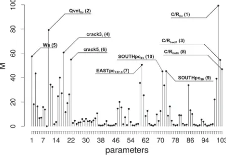
The results from preliminary FS are depicted in Figure5, where the first-order effects calculated from the Morris method (Mi indexes) are shown. In particular, the 10 most important model parameters are highlighted.C/Rliv and Qvntliv are the two most influential variables fol-lowed by Ws, crack3l, crack5l, EASTpc157.5, SOUTHpc90, SOUTHpc45,C/Rbed1 andC/Rbathwhich have very simi-larMiindexes. These 10 factors have been labelled as MIF and grouped according to the phenomena they represent:
• C/Rliv,C/Rbed1 C/Rbath have been collected in the
C/Rparameter;
• EASTpc157.5, SOUTHpc90, SOUTHpc45 have been gathered in the PC parameter;
• crack3l and crack5l have been grouped in the CRACK parameter;
[image:14.610.322.546.559.713.2]while Qvntlivand Ws have been considered separately.
From the results from FF it is also possible to iden-tify the wind direction most influencing the Twin House O5. By rotating the pressure coefficients azimuth angles, in order to refer to the same reference direction, north, the wind coming from direction within the range [225◦, 270◦] seems to have the largest effects on the internal tempera-tures.
6.2. FF and FP
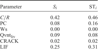
The first-order (Si) and total effects (STi) are listed in Table 3. The model is mainly dominated by first-order effects as the small differences betweenSi and STi indi-cate. In particular, the sum of the first-order effects is equal to 86% ofV(T)meaning that about the 14% ofV(T)is due to higher order effects. Most of the higher order effects can be attributed to interactions between PC and LIF. They are the only two groups having a noticeable difference between their STiandSi.
In the light of this consideration, the higher order effects between the defined group of parameters are negligible. For the total variance, 61% can be attributed to the MIF (most of which is attributable toC/R), 25% to the LIF and about 14% to interactions, occurring especially between PC and LIF. Thus even if MIF account for the majority of the model variance, still one-third of it is determined by less important factors and their approximation to default values should be undertaken with caution.
6.3. Factor mapping
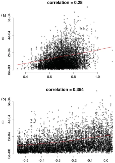
[image:15.610.319.549.67.530.2]The model did not provide a particularly good fit of the measured data. In particular, it was able to provide rea-sonable predictions in the middle part of the ROLBS experiment, but at the beginning and at the end of the heating sequence the simulation outcomes overestimated the observed internal temperatures. This trend is noticeable especially for the living room (Figure6(a)), while for the bedroom 1 (Figure6(b)) and the bathroom (Figure6(c)) the discrepancies between model outputs and measurements are less evident. The main causes are probably model deficiencies lying in the analysed sub-models or in other parts of the overall BES model. In this study, they were investigated by calculating the Pearson correlation coef-ficient between the residuals and multidimensional model
Table 3. First-order (Si) and total effects (STi) from the Sobol methods forT.
Parameter Si STi
C/R 0.42 0.46
PC 0.08 0.16
Ws 0.00 0.00
Qvntliv 0.09 0.08
CRACK 0.02 0.02
LIF 0.25 0.31
(a)
(b)
(c)
Figure 6. Comparison between model predictions (black) and observed temperatures (red) (in colour online).
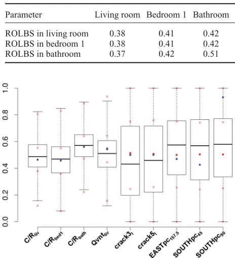
inputs, showing that ROLBS sequences and residuals were moderately correlated (Table 4). The analysis has thus identified an aspect of the model and/or program that needs to be improved in order to get a better match with the measured data.
[image:15.610.97.261.642.729.2]Table 4. Correlation between residuals and ROLBS heating sequences.
Parameter Living room Bedroom 1 Bathroom
ROLBS in living room 0.38 0.41 0.42
ROLBS in bedroom 1 0.38 0.41 0.42
ROLBS in bathroom 0.37 0.42 0.51
[image:16.610.319.548.416.685.2]Figure 7. Comparison between prior (red crosses: quartiles, red dots: averages, blue dots: initial values) and posterior (box-plot) parameter distributions, for MIF. The samples have been normalized between 0 and 1 (in colour online).
Table 5. Posterior estimates and 95% confidence intervals. Parameter Units Posterior estimate 95% CI
C/Rliv – 0.72 0.53 0.90
C/Rbed1 – 0.71 0.50 0.90
C/Rbath – 0.71 0.52 0.90
Qvntliv m3/h 59.4 54 61.2
crack3l m 1.91 0.85 3.12
crack5l m 1.93 0.87 3.14
EASTpc157.5 – −0.20 −0.84 0.32
SOUTHpc45 – −0.04 −0.56 0.40
SOUTHpc90 – −0.36 −0.97 0.16
the same there are shifts between prior and posterior esti-mates. The threeC/Rratios have estimates very close to their initial values, especiallyC/Rbed1 andC/Rbath, while
C/Rliv assumes a value slightly higher. Similar consid-erations can be drawn for the inflow ventilation rate. Its posterior value, although slightly lower, is substantially in agreement with the one inferred from the data. More signif-icant variations between prior and posterior estimates can be observed for crack parameters and pressure coefficients, especially for the latter. Crack lengths assume values about 4% lower than the initial model considered. Pres-sure coefficients move sensibly from their initial values: EASTpc157.5increases by 44%, SOUTHpc45decreases by 89% and SOUTHpc90increases by 28%.
One possible cause of significant posterior variance for crack lengths and pressure coefficients can be over-parametrization of the model. This aspect has been anal-ysed by applying the Sobol method to the calculated weights (Table6). The variance of the weighting function is mostly due to PC and LIF. This is unexpected since the results from FF and FP were showing thatC/Rcoefficients were responsible by themselves for 42% of the model vari-ance. Additive and linear effects account for the 75% of V(ωωω), so that the remaining 25% can be attributed to higher order effects mainly due to PC and LIF.
These results indicate that among the LIF there are parameters important for model calibration and validation. Such variables can be identified by comparing their prior and posterior distributions in the same way as was done for the MIF. LIF factors showing significant differences are likely to contribute in a relevant manner to a bet-ter match with the measurements. Such comparison is shown in Figure8 where the variables having the larger differences between their prior and posterior averages are highlighted. These parameters are crack2w, crack2l, EASTpc135, SOUTHpc67.5and WESTpc337.5.
It can also be useful to analyse scatter plots of ωωω against the posterior parameter samples and calculate the correlation between them. In this way, it is possible to
Table 6. First-order (Si) and total effects (STi) from the Sobol method relative toωi.
Parameter Si STi
C/R 0.06 0.08
PC 0.20 0.39
Ws 0.00 0.00
Qvntliv 0.08 0.12
CRACK 0.04 0.07
LIF 0.37 0.49
[image:16.610.62.297.423.543.2]