City, University of London Institutional Repository
Citation:
Broom, M., Johanis, M. and Rychtar, J. (2014). The effect of fight cost structure
on fighting behaviour. Journal of Mathematical Biology, pp. 979-996. doi:
10.1007/s00285-014-0848-x
This is the accepted version of the paper.
This version of the publication may differ from the final published
version.
Permanent repository link:
http://openaccess.city.ac.uk/5125/
Link to published version:
http://dx.doi.org/10.1007/s00285-014-0848-x
Copyright and reuse: City Research Online aims to make research
outputs of City, University of London available to a wider audience.
Copyright and Moral Rights remain with the author(s) and/or copyright
holders. URLs from City Research Online may be freely distributed and
linked to.
City Research Online:
http://openaccess.city.ac.uk/
[email protected]
(will be inserted by the editor)
The effect of fight cost structure on fighting behaviour
Mark Broom · Michal Johanis · Jan Rycht´aˇr
Received: date / Accepted: date
Abstract A common feature of animal populations is the stealing by animals of re-sources such as food from other animals. This has previously been the subject of a range of modelling approaches, one of which is the so called “producer-scrounger” model. In this model a producer finds a resource that takes some time to be consumed, and some time later a (generally) conspecific scrounger discovers the producer with its resource and potentially attempts to steal it. In this paper we consider a variant of this scenario where each individual can choose to invest an amount of energy into this contest, and the level of investment of each individual determines the probability of it winning the contest, but also the additional cost it has to bear. We analyse the model for a specific set of cost functions and maximum investment levels and show how the evolutionarily stable behaviour depends upon them. In particular we see that for high levels of maximum investment, the producer keeps the resource without a fight for concave cost functions, but for convex functions the scrounger obtains the resource (albeit at some cost).
Keywords kleptoparasitism·sequential game·extensive form game·food stealing· game theory
Mark Broom
Department of Mathematics, City University London, Northampton Square, London, EC1V 0HB, UK E-mail: [email protected]
Michal Johanis
Department of Mathematical Analysis, Charles University, Sokolovsk´a 83, 186 75 Praha 8, Czech Republic E-mail: [email protected]
Jan Rycht´aˇr
Department of Mathematics and Statistics, The University of North Carolina at Greensboro, Greensboro, NC 27412, USA
1 Introduction
Animals need a variety of resources to live and reproduce, and often they have to com-pete with other animals for them. These resources include territories, mates and food. Their competitors can be conspecifics or member of other species, and the nature of contests vary depending upon the animals involved and the resources competed over. Territories are often of value for a significant period of time, if not indefinitely, and so provide significant opportunities for contests over ownership, with a series of intruders (Kruuk, 1972; Hamilton and Dill, 2003; Iyengar, 2008; Kokko, 2013).
Food resources however are often only available for small periods. If a food item can be consumed immediately by the individual that discovered it, then there is gen-erally no chance for another to compete for it. Often, however, food items require a non-trivial handling time to eat them. This can be because the food item is destined for the offspring of the individual, and some must be transported to the nest or den, during which time others have the opportunity of taking it. Alternatively, it might take a while to consume because it has a tough exterior that needs to be penetrated, like a shell, or needs to be consumed in pieces which requires a bird to land to eat it (Spear et al, 1999; Steele and Hockey, 1995; Triplet et al, 1999). Such scenarios have been modelled by Broom and Ruxton (2003); Broom et al (2004); Broom and Rycht´aˇr (2007); Broom et al (2008); Broom and Rycht´aˇr (2011). Alternatively the resource might be a large food patch which just takes time to completely consume, which is the focus of producer-scrounger models (Barnard and Sibly, 1981; Barnard, 1984; Caraco and Giraldeau, 1991; Vickery et al, 1991; Dubois and Giraldeau, 2005), see also Giraldeau and Livoreil (1998); Kokko (2013); Broom and Rycht´aˇr (2013) for more general reviews.
2 The Model
We model the situation described above as a game in extensive form. One individ-ual, a producer, is in possession of a resource of fixed valuev. Another individual, a scrounger, comes along and may attempt to steal it. The scrounger investss∈[0, S]
units of energy in the stealing attempt. Whens= 0, nothing happens. Whens >0, the producer then investsp∈[0, P]units of energy in defending the item. The prob-ability that the producer successfully defends the item will be an increasing function ofp, and a decreasing function ofs, which for tractability of analysis we simply set as s+pp. Such a function has been introduced in Tullock (1980), who considered the
more general formskp+kpk, which in the limit ofk→ ∞gives the case where the
in-dividual with the highest investment always wins, as in the classical war of attrition, e.g. see Bishop and Cannings (1978). Such functions were axiomatized by Skaperdas (1996), and our natural choice has now become widely used (see for example Con-gleton et al, 2008). When the individuals engage in the fight, each one incurs a cost
c(s, p).
In full generality, the cost function c(s, p)is asymmetrical and potentially dif-ferent for the scrounger and producer. It consists of the true energetic cost of the investment (such as performing a complex manoeuvre in an aerial contest between birds), the potential for getting hurt by an animal’s own actions (typically, the more complex the manoeuver, the more things could go wrong and the animal could end up seriously injured even if the other individual does not fight) and the potential for getting hurt by the actions of the opponent. However, in such a full generality, the mathematics would be intractable, and we thus consider a symmetrical cost function (note that it is possible to find solutions for linear asymmetric functions, as shown in Baye et al (2012)). The symmetrical cost function that we use is defined by
c(s, p) = (s+p)α (1)
fors+p >0andα≥0. We note that one consequence of this is that extra investment by the other player will directly affect an individual’s cost, and so potentially its chosen strategy. Clearly we do not need to define the cost ats+p = 0, since a contested resource requiress >0andp≥0. We note that there are other symmetrical cost functions used, such as min(p, s)in the war of attrition, where effort corresponds to the time an individual is prepared to wait in a purely passive contest, so that the extra time over and above when the other individual concedes does not need to be spent.
scrounger
producer
Fight
scrounger wins
producer wins
producer gives up
scrounger gives up
scrounger’s payoff producer’s payoff
−(s+p)α+v −(s+p)α−v
−(s+p)α −(s+p)α
−sα+v −sα−v
0 0
s >0
s= 0 p >0
p= 0 s s+p
p s+p
Fig. 1: Scheme of the game. First, the scrounger invests s ∈ [0, S]. Ifs > 0, the producer then investsp ∈ [0, P]. Ifp > 0, there is a fight that the scrounger wins with probabilitys/(s+p). Both individuals pay the costs, the winner of the contest keeps the resource that was originally in the possession of the producer.
of its own and some of the other player’s effort costs). Nested in their model is the casec(s, p) =s+p, which is also a special case considered in this paper.
Note that the cost is a function ofs+p, which means that the producer pays the cost even if it does not engage in the fight. This is a plausible outcome under a variety of scenarios. For example, the producer may be hurt by the scrounger’s attack even if the producer does not invest anything in fighting back. Similarly, if the producer does not want to fight, it may need to flee the scene and the energy expenditure of doing so may be correlated with the strength of the scrounger’s attack. Finally, the cost may be interpreted as damage to the environment; for example any kind of attack on a fishing bird may scare away any potential fish and reduce its medium gain from fishing.
It is worth considering what circumstances are likely to lead to the different types of cost function, i.e. the different values of the parameterα. It seems reasonable that as the effort involved increases, the duration of the contest will increase sublinearly and the risk of injury and fitness costs due to lost energy will increase supralinearly. Thus if the major cost is due to risk of injury or lost energy,αis likely to be greater than1, i.e. we have a convex function, whereas if time costs are the biggest problem, for example if this is due to exposure to predation risk, then we haveαless than1, i.e. a concave function.
We will study how the stealing behaviour can evolve for different values of the parameterα. When0 < α < 1, then even a small investment in the fight is rel-atively costly, but enlarging an already large investment is relrel-atively inexpensive.
Whenα >1, then small investments in the fight are cheap, but enlarging an already
large investment is very costly. Whenα= 0, the cost of the fight is constant regard-less of the investment for any contested resource (i.e. for anys >0).
Usfor the producer and scrounger will thus be
Up(s, p) =−(s+p)α−v s
s+p, (2)
Us(s, p) =−(s+p)α+v s
s+p, (3)
whenevers+p >0and
Up(0,0) =Us(0,0) = 0. (4)
The game is shown in Figure 1.
3 Analysis
In each case that we analyse below, the scrounger will make an initial choice ofs, and then the producer will pick a valuep(s)which may vary depending upon the value ofsactually encountered. Thus any strategy will be a choice of a single number for the scrounger, and a function of all possible encountered scrounger strategies for the producer. This will result in a realisation of the producer’s strategy which is the actual value of its function for the chosen value ofs, but it should be borne in mind that the producer’s strategy is the response function, not just the single number (see the text at the end of Section 4.3).
3.1 Caseα= 0
Let us first examine the special case ofα= 0, i.e. a constant fight cost.
Assume the scrounger attempted to steal(s >0). The payoff to the producer will then be
Up(s, p) =−1−v s
s+p. (5)
Since ∂Up
∂p >0, it is optimal for the producer to fight with maximal intensityP.
If the scrounger does not attack (s = 0), its payoff will be0. If the scrounger attacks (s >0), we also get∂Us
∂s >0, so that the scrounger should invest the maximal
valueSin the fight. Hence, putting it together with the producer’s optimal decision, the maximal scrounger’s payoff fors >0is−1 +vS/(S+P).
3.2 Caseα >0.
For a givens≥0we find an optimal response of the producer. Clearly, whens= 0, the producer’s response isp0(0) = 0.
For a fixeds∈(0,+∞)we have
∂Up
∂p (s, p) =−α(s+p)
α−1+ vs
(s+p)2, (6)
which holds forp∈(−s,+∞)(clearlyp <0andp > P do not correspond to real solutions as they fall outside the valid range, yet it is mathematically convenient to consider all values ofpat this stage) and is continuous there. The critical points of the functionp7→Up(s, p), i.e. the pointspwhere∂Up
∂p (s, p) = 0, are given by
p=g(s) =vs
α
α+11
−s. (7)
Note thatg(s) > −swhens > 0. For convenience, we continuously extendgby settingg(0) = 0. Furthermore,
∂2U p
∂p2 (s, g(s)) = −α(α−1)(s+p) α−2
−(s2+vsp)3
(s,g(s))
(8)
=−α(α+ 1)vs
α
αα−2+1
<0. (9)
It follows that ∂Up
∂p (s, p) > 0 for p ∈ (−s, g(s)) and ∂Up
∂p (s, p) < 0 for p ∈ (g(s),+∞). Consequently,p 7→ Up(s, p)is increasing on(−s, g(s)]and decreas-ing on[g(s),+∞)(and attains its unique maximum on(−s,+∞)atg(s)). However, we have to maximisep7→Up(s, p)on[0, P]. Thusp7→Up(s, p)attains its unique maximum on[0, P]at
p0(s) =
0 ifg(s)≤0,
P ifg(s)≥P,
g(s) otherwise.
(10)
Note thatp0(s) = max0,min{g(s), P} and it is a continuous function on[0,+∞).
Recall thatg(0) = 0, and, by (7), fors >0we haveg(s)≤0if and only if
s≥c4:=
v
α
α1
. (11)
Further,
g0(x) = 1
α+ 1
v
α
α+11
x−αα+1−1, (12)
g00(x) =−(α+ 1)α 2
v
α
α+11
0 0.5 1 1.5 2 2.5 0 0.2 0.4 0.6 0.8 1 s
Producer’s optimal response
v=5 v=10 v=25 v=50 v=100 (a)
0 2 4 6 8
0 0.2 0.4 0.6 0.8 1 s
Producer’s optimal response
v=2 v=3 v=4 v=5 v=6 (b)
0 2 4 6 8 10 0 0.2 0.4 0.6 0.8 1 s
Producer’s optimal response
[image:8.595.76.410.74.186.2]v=1 v=2 v=3 v=4 v=5 (c)
Fig. 2: Producer’s optimal responses to varying scrounger’s investment levelsand different values ofvforP = 1. (a)α= 4, (b)α= 1, (c)α= 0.8.
forx∈(0,+∞). Thusgis strictly concave on(0,+∞). Sinceg0(x) = 0if and only
if
x=c1:=
1 (α+ 1)α+1α
v
α
α1
>0, (14)
the functiong attains its unique maximum on(0,+∞)atc1. It follows that the
in-equalityg(s)≥P has a solution if and only if
P ≤g(c1) =c3:=
1−α+ 11
1 (α+ 1)α1
v
α
α1
; (15)
moreover, asg(0) = 0< P andgis strictly concave on(0,∞), there exist constants
a(P), b(P)satisfying0< a(P)≤b(P)< c4and such thatg(s)≥P if and only if
s∈[a(P), b(P)]. The producer’s optimal responses are shown in Figure 2.
To find the optimal strategy for the scrounger we have to maximise the scrounger’s payoff given the producer responds optimally, i.e. the function
f(s) =Us(s, p0(s)). (16)
We define
h(s) =Us(s, P) =−(s+P)α+ vs
s+P, (17)
and then we have
f(s) =
0 ifs= 0,
−sα+v ifs > c
4, i.e.p0(s) = 0,
h(s) ifP ≤c3ands∈[a(P), b(P)], i.e.p0(s) =P, (α−1) vs
α
αα+1 otherwise, i.e.p
0(s) =g(s).
(18) We note thatf is a continuous function on[0,+∞). We have
h0(x) =−α(x+P)α−1+ vP
(x+P)2, (19)
h00(x) =−α(α−1)(x+P)α−2
Notation Meaning
S the upper limit of the scrounger’s investment in the fight
P the upper limit of the producer’s investment in the fight
α the indicator of the concavity of the cost function
v the value of the contested resource
Up(s, p) payoff to the producer when the scrounger playssand the producer playsp
Us(s, p) payoff to the scrounger when the scrounger playssand the producer playsp
p0(s) the optimal response of the producer given the scrounger playeds
f(s) Us(s, p0(s)), i.e. an anticipated scrounger’s payoff when playingsand the producer responds optimally
h(s) Us(s, P), i.e. the scrounger’s payoff when scrounger playssand producer playsP
g(s) critical point of the producer’s payoff function (and thus a candidate for the optimal response) if the scrounger playeds g(P) critical point of the scrounger’s payoff functionh(s)(if producer’s effort is locally fixed atP
a(P), b(P) solutions ofg(s) =P;g(s)≥Pif and only ifs∈[a(P), b(P)],p0(s) =Pon[a(P), b(P)]
c1 the point whereg(s)attains its maximum
c2 the point whereg(g(s)) =s;g(P)∈[a(P), b(P)]if and only ifP ≤c2
c3 the maximal value ofg, i.e.c3=g(c1)
c4 the point whereg= 0;g(s)<0if and only ifs > c4
c0 the point whereh(g(p)) = 0;h(g(P))>0if and only ifP < c0
k(P) a solution off(s) =f(g(P))that lies in the interval[b(P), c4)
[image:9.595.74.513.66.280.2]l(S) a solution ofUs(S, x) = 0
Table 1: Notations used in the manuscript.S, P, α, vare parameters of the model.
forx∈(−P,+∞). Note thath0(x) = 0if and only ifx=g(P)and thatg(P)>
−P. Since h0(g(P)) = 0andh00(g(P)) = −α(α+ 1) vP α
αα−2+1 < 0, it follows
that h0 > 0 andh is increasing on (−P, g(P)] andh0 < 0 andhis decreasing
on[g(P),+∞). The behaviour ofhon[a(P), b(P)]depends on whetherg(P) ∈
[a(P), b(P)], i.e.g(g(P))≥P. This happens if and only if
P ≤c2:= 1
2
v
2α
α1
. (21)
Note thatgrepresents a critical point of either player’s payoff function if the other player’s effort is effectively locally fixed. In a region where the producer’s effort is locally fixed at P, such that marginal changes in the scrounger’s effort do not change the producer’s effort, the scrounger’s payofff(s)is given byh(s)and since
h0(g(P)) = 0(withg(P)being the only root ofh0),g(P)describes a critical point
of the scrounger’s payoff function.
4 Results
Now we distinguish three cases.
4.1 Caseα >1
Note that in this case c1 < c2 < c3 < c4. If P > c2, then f is increasing on [0, c4](this follows from the fact thathis monotone on[a(P), b(P)]andf(a(P))<
0
0 c
1
c1
c2
c2
c3
c3
c4
c4
P S
v v
(S, P)
g(P) k(P)
g(S) (S, g(S))
(g(P), P)
[image:10.595.117.338.83.288.2](c4,0)
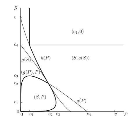
Fig. 3: Different types of equilibria forα = 4, fixed v and varyingS andP. The bold lines are the boundaries of the regions where types of the equilibrium types change. The equations for curvesgandkare given in (7) and (22). The figure looks same for all values ofv because the constantsc1, . . . , c4 and the functiong(P) =
v1/αh P
αv1/α
α+11
− P v1/α
i
and thus also a functionk(P)scale appropriately by a
factorv1/α. The situation is analogous for anyα >1.
unique maximum on[0, S]atS, while ifS≥c4, thenfattains its unique maximum
on[0, S]atc4.
IfP ≤c2< c3, thenf is increasing on[0, g(P)], decreasing on[g(P), b(P)],
in-creasing on[b(P), c4], and decreasing on[c4,+∞). We havef(g(P)) =h(g(P)) =
v−(α+ 1) vP
α
αα+1 andf(c
4) = −cα4 +v = v−αv. Thusf(g(P)) > f(c4)if
and only ifP < c1. Therefore in this case ifS < g(P), thenf attains its unique
maximum on[0, S]atS, while ifS ≥g(P), thenf attains its unique maximum on
[0, S]atg(P). Finally, ifc1 ≤ P ≤ c2, then there isk(P) ∈ [b(P), c4)such that
f(k(P)) =f(g(P)). This is given by
k(P) = 1
(α−1)α+1α
α
v v−(α+ 1)
vP
α
αα+1!
α+1
α
The following summary is then easily deduced:
P > c2
(
S < c4 maximum atS,
S≥c4 maximum atc4,
c1≤P ≤c2
S < g(P) maximum atS,
g(P)≤S < k(P) maximum atg(P),
k(P)≤S < c4 maximum atS,
S≥c4 maximum atc4,
P < c1
(
S < g(P) maximum atS,
S≥g(P) maximum atg(P).
(23)
It means that the scrounger will play eitherc4, g(P)or S. The corresponding
re-sponses by the producer will bep0(c4) = 0,p0(g(P)) = P (becauseP ≤c2) and
p0(S) =
(
P, ifg(S)≥P ,
g(S), otherwise. (24)
The situation is summarised on Figure 3. We note that sendingS andP to infinity corresponds to the situation where there is no upper bound on the investments possi-ble, and here this leads to the solution(c4,0), where the scrounger steals the resource
with no resistance from the producer.
It should also be noted that in this and later sections, sendingvto 0 has similar effects to sendingS andP to infinity, since although for finite S andP there are theoretical limits on the energy that can be invested, for smallvthe energy that any individual would invest in practice is also small.
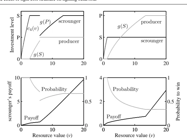
The equilibrium investments and resulting payoffs for fixedSandP and varying
vare shown in Figure 4. Also, note the discontinuity of the strategies whenS > P. This happens for all values ofαand is caused by the switch from one solution to another, when crossing from the (S, g(S))region to the(g(P), P)region. We can see that only the probabilities and not the payoffs are discontinuous. Thus, here we see one example of a well known fact that the maximum of the function is continuous as the parameter changes but the maximizer may not be continuous (Berge, 1963).
To examine the phenomenon in more details, let us directly examine the connec-tions between Figures 3 and 4. For fixed valuesSandP(sayS= 2andP= 1) and a temporarily fixed valuev, the point with coordinates[P, S]falls into a specific region in Figure 3. Asv grows, the regions in Figure 3 grow as well (without essentially changing shape) while the point[P, S]remains fixed. Hence the point that was origi-nally in the(c4,0)region (such as the one for small values ofv) eventually falls into
the(S, g(S))region (this a continuous, but not differentiable change of optimal in-vestment level). Asvgrows even further, the same point then falls into the(g(P), P)
region (indicating a discontinuous change or a jump of optimal investment level). As
vgrows even more, the point then finally falls into the(S, P)region.
0 10 20 0
S P
g(S)
scrounger producer
0 10 20
0 2 4
Resource value (v) Probability
Payoff
0 10 200
0.5 1
Probability to win
0 10 20
0 P S
Investment level
c4(v)
g(S)
g(P) scrounger
producer
0 10 20
0 5 10
scrounger’s payoff
Resource value (v) Probability
Payoff
0 10 200
[image:12.595.80.398.73.310.2]0.5 1
Fig. 4: Equilibrium investment levels for the scrounger and producer and the scrounger’s payoffs and probability of victory when (a)S = 2,P = 1,α = 1.2
(left column) and (b)S = 1, P = 2, α= 1.2(right column) are fixed. We note that
gis in fact a functiong(x) = gα,v(x) = vx α
α+11
−x. In this figure,g(S)means a functionv7→gα,v(S), andg(P)is interpreted analogously.
more but it cannot because it has reached its maximum already, and thus it becomes beneficial for the producer to invest (it improves the odds of winning the fight and the increase of the reward value outweighs the cost associated with the investment). Asvcontinues to grow, the producer invests more and more and since the scrounger cannot invest more thanS, its odds of winning decrease and at one point, the odds decrease so much that the reward does not justify the cost and it becomes beneficial to invest less than maximum.
4.2 Caseα= 1
Note that in this case c1 = c2 = c3 = v/4 < c4 = v. If P ≥ c1 thenf is
zero on[0, c4]. IfP < c1, thenf is zero on[0, a(P)]and[b(P), c4], increasing on [a(P), g(P)]and decreasing on[g(P), b(P)]. Therefore we obtain
P ≥c1
(
S < c4 maximum anywhere in[0, S],
S≥c4 maximum anywhere in[0, c4],
P < c1
S ≤a(P) maximum anywhere in[0, S], a(P)< S < g(P) maximum atS,
S ≥g(P) maximum atg(P).
0
0 c
1=v/4
c1
c4=v
c4=v
P S
(S, P) g(P)
g(S)
(s, g(s)) for anys∈[0, S]
(g(P), P)
(s, g(s)) for anys∈[0, c4]
0
0 c
1=v/4
c1
c4=v
c4=v
P S
(S, P) g(P)
g(S)
(s, g(s)) for anys∈[0, S]
(g(P), P)
[image:13.595.81.342.72.275.2](s, g(s)) for anys∈[0, c4]
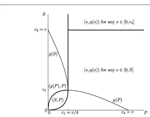
Fig. 5: Different types of equilibria forα= 1, fixedvand varyingSandP. The bold lines are the boundaries of the regions where types of the equilibrium types change. The equation for the curvegis given in (7). The scrounger can chose from multiple equilibria. Note that the graph ofa(P)coincides with the lower branch of the graph ofg(S)becausea(P)is the smaller solution ofP =g(s).
This means that the scrounger will play eitherg(P),S, anything between0and
c4, or anything between0andS. The corresponding responses by the producer will be
p0(g(P)) =P(becauseP ≤c2=c1),p0(S) =P(becauseg(S)≥P) andp0(s) =
g(s)in the remaining cases. The situation is summarised in Figure 5. Here sending
S andP to infinity leads to a solution of the form (s, g(s)), where the resource is contested by both parties.
The equilibrium investments and resulting payoffs for fixedSandP and varying
vare shown in Figure 6.
We note that there are large ranges of the scrounger’s investment level which give the same maximum payoff of0 to the scrounger. This can be seen directly by substituting into the formula
f(s) =Us(s, p0(s)) =−(s+p0(s)) +v
s s+p0(s)
(26)
=−(s+√vs−s) +v s
s+√vs−s = 0 (27)
for the large range ofsvalues wherep0(s) =g(s).
4.3 Caseα <1
Note that in this casec2< c3< c1< c4. IfP > c2, thenfis decreasing on[0,+∞)
0 5 10 0
S P
c3(v)
scrounger producer
0 5 10
0 0.2 0.4 0.6 0.8 1
Resource value (v) Probability
Payoff
0 5 10 0
0.5 1
Probability to win
0 5 10
0 P S
Investment level
c4(v)
c3(v) g(P)
scrounger
producer
0 5 10
0 5
scrounger’s payoff
Resource value (v) Probability
Payoff
0 5 10 0
[image:14.595.80.399.74.314.2]0.5 1
Fig. 6: Equilibrium investment levels for the scrounger and producer and the scrounger’s payoffs and probability of victory when (a)S = 2, P = 1, α = 1
(left column) and (b) S = 1, P = 2, α = 1 (right column) are fixed. Here, the scrounger has a choice for anysin the black and darker gray region, the producer then replies byp=g(s)which falls in the darker or lighter gray region. Probability of scrounger’s victory depends on the scrounger’s strategy, the maximal probability (corresponding to maximal optimal investment level) is shown.
f(a(P)) > f(b(P))by continuity) and so it attains its unique maximum on[0, S]
at0. IfP ≤c2, thenf is decreasing on[0, a(P)], increasing on[a(P), g(P)], and
decreasing on [g(P),+∞). Thusf still attains its maximum on[0, S] at0 unless
h(g(P))>0, which happens if and only if
P < c0:=
α
α+ 1
α+1α v
α
α1
< c2. (28)
In this case we need to know whetherSlies in the interval wherehis positive. We define
l(S) = (vS)α+11 −S. (29)
Note thath(S)>0if and only if
0
0 c
0
c0
g(c0)
v v
P S
(S, P)
g(P) l(S)
(0,0)
[image:15.595.129.336.77.279.2](g(P), P)
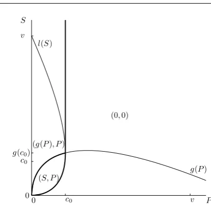
Fig. 7: Different types of equilibria forα= 0.8, fixedv and varyingS andP. The bold lines are the boundaries of the regions where types of the equilibrium types change. The equations for curvesgandl are given in (7) and (30). The situation is analogous for anyα <1.
Thus we may conclude that
P ≥c0 maximum at0,
P < c0
S ≤g(P)andP ≥l(S) maximum at0,
S ≤g(P)andP < l(S) maximum atS,
S > g(P) maximum atg(P).
(31)
This means that the scrounger will choose to play either0,S org(P). The corre-sponding responses by the producer will bep0(0) = 0,p0(S) =P (because in this
caseP < l(S)< g(S)) andp0(g(P)) =P(because in this caseP < c0< c2). The
situation is summarised in Figure 7. SendingSandP to infinity here yields the so-lution of (0,0), with the scrounger not challenging for the resource in the unbounded investment case. This may seem a counterintuitive result because it appears that the scrounger would be better off playings >0and then gaining a reward for a little cost (after the producer gives up by playingp= 0). However,p= 0is just the realisation of the actual producer’s strategy, which is to play a specific function ofp0(s)given
by (10), against whicheversoccurs. For α < 1, whens > 0, then the producer’s best reply isg(s)(at least in the case whenP is large), which would yield a negative payoff to the scrounger, and hence the scrounger should indeed play0.
The equilibrium investments and resulting payoffs for fixedSandP and varying
0 5 10 0
S P
scrounger producer
0 5 10
0 0.5 1
Resource value (v) Probability
Payoff
0 5 100
0.5 1
Probability to win
0 5 10
0 P S
Investment level
g(P) scrounger
producer
0 5 10
0 2 4
scrounger’s payoff
Resource value (v) Probability
Payoff
0 5 100
[image:16.595.80.399.74.314.2]0.5 1
Fig. 8: Equilibrium investment levels for the scrounger and producer and the scrounger’s payoffs and probability of victory when (a)S = 2,P = 1,α = 0.8
(left column) and (b)S= 1, P = 2, α= 0.8(right column) are fixed.
5 Discussion
Previous game-theoretical models of food stealing behaviour Broom and Ruxton (2003); Broom et al (2004); Broom and Rycht´aˇr (2007); Broom et al (2008); Broom and Rycht´aˇr (2011) have considered a number of different scenarios for when an an-imal tries to gain resources by stealing, rather than by directly acquiring them itself. Typically these models only consider a small range of options for the players in-volved, for example to attempt to steal or not (Crowe et al, 2009; Broom et al, 2013, 2014), or play Hawk or Dove in a contest Broom et al (2009); Grundman et al (2009). Such a discrete set of options is commonly considered in wider ecological scenarios, for example patch foraging, where the choice may be to forage on a particular patch (Fretwell and Lucas, 1970; Kˇrivan et al, 2008). In many real situations, individuals will have a greater flexibility of options, for example forage for a while and then move to a different patch (Charnov, 1976). We also note that our model can be applied be-yond biological sciences, such as to quantity-setting games in economics between two firms (Varian and Repcheck, 2005, Ch. 27).
energy reserves. However, the bigger the investment in the contest, the bigger the chances of winning, but also the bigger the costs of the potential contest. This creates another trade-off situation for the individuals. This is the situation that we consider in this paper: related models from economics have been considered, for example in Tullock (1980); Baye et al (2012); Skaperdas (1992). We note that the role of budget limits has been analysed, see for example Che and Gale (1997); Bester and Konrad (2004), and plays a crucial role in Colonel Blotto games (Roberson, 2006).
We have shown that when maximum investment levels are low or equivalently whenvis large compared to the maximum investment levels, generally both animals should play at the maximum level. However, when they are high orvis not too large, then the equilibria depend greatly upon the nature of the cost function. For a convex function the scrounger can find a sufficient investment level (but one not too high to be profitable) to force the producer to concede. For a concave function the scrounger will not challenge, so the producer keeps the resource with no investment. Only at the boundary linear case will there be a contest for the resource.
If the individuals do not have the same maximum level, we saw that the situation is typically more favourable to the individual with higher maximum. WhenS > P, then the scrounger always invests more than the producer and obtains a favourable payoff. WhenP > S, then the producer invests more than the scrounger for large values ofv. Interestingly, as seen at Figure 4b, when the payoff is convex,P > S
andv is relatively small (but not too small), then a scrounger invests more than a producer (and is thus likely to win the fight). Still, regardless of the convexity of the payoff function, whenP > Sthe scrounger’s payoff is small (relatively to the value ofv).
As we have seen, the order of the players in such a sequential game can make a real difference. We have assumed that the scrounger is the first player and the pro-ducer is the second. This makes sense, as usually the propro-ducer will be in control of a stationary resource and the scrounger will have to make the first move. However, there may be situations where the reverse is true, for example if the resource is suffi-ciently large or spread out that an active defence is required to chase off an intruder. In this case, the results that we have obtained for producer and scrounger would be swapped. There may also be circumstances where the game can be assumed to be one involving simultaneous decisions (as in the earlier models, such as Barnard (1984)), which would require a different game-theoretical model. See for example McNamara et al (2006) where authors study the differences between the two approaches for a similar game.
already obtained will occur, where (in the absence of energy limits) one individual will concede. However, with uncertainty, there will likely be more contests where both individuals fight.
Note that we have also used rather simplistic functions for both the probability of victory, and the cost of the contest. These were for reasons of mathematical tractabil-ity. It is possible to consider alternative forms for each of these functions. Similarly the costs, the probability of victory and the maximum energy investment of the an-imals may all depend upon some property of the animal, for example its Resource Holding Potential, see for example Hurd (2006). These could be considered in later versions of the model. The main rationale for this paper, however, was to introduce the concept of energetic investment into food stealing contests, as well as to show some of its effects, and as mentioned earlier there is a significant range of existing models where this kind of idea could be applied.
Acknowledgements
The research has been supported by grant GA ˇCR 201/11/0345 (Michal Johanis) and the Simons Foundation grant #245400 (Jan Rycht´aˇr).
References
Barnard C (1984) Producers and scroungers: strategies of exploitation and parasitism. Springer
Barnard C, Sibly R (1981) Producers and scroungers: a general model and its appli-cation to captive flocks of house sparrows. Animal Behaviour 29(2):543–550 Baye MR, Kovenock D, de Vries CG (2005) Comparative analysis of litigation
sys-tems: An auction-theoretic approach*. The Economic Journal 115(505):583–601 Baye MR, Kovenock D, de Vries CG (2012) Contests with rank-order spillovers.
Economic Theory 51(2):315–350
Berge C (1963) Topological Spaces: including a treatment of multi-valued functions, vector spaces, and convexity. Dover Publications
Bester H, Konrad KA (2004) Delay in contests. European Economic Review 48(5):1169–1178
Bishop D, Cannings C (1978) A generalized war of attrition. Journal of Theoretical Biology 70(1):85–124
Broom M, Ruxton G (2003) Evolutionarily stable kleptoparasitism: consequences of different prey types. Behavioral Ecology 14(1):23
Broom M, Rycht´aˇr J (2007) The evolution of a kleptoparasitic system under adaptive dynamics. Journal of Mathematical Biology 54(2):151–177
Broom M, Rycht´aˇr J (2011) Kleptoparasitic meleesmodelling food stealing featuring contests with multiple individuals. Bulletin of Mathematical Biology 73(3):683– 699
Broom M, Rycht´aˇr J (2013) Game-theoretical models in biology. CRC Press Broom M, Luther R, Ruxton G (2004) Resistance is useless? - extensions to the game
Broom M, Luther RM, Ruxton GD, Rycht´aˇr J (2008) A game-theoretic model of kleptoparasitic behavior in polymorphic populations. Journal of Theoretical Biol-ogy 255(1):81–91
Broom M, Luther RM, Rycht´aˇr J (2009) A hawk-dove game in kleptoparasitic popu-lations. Journal of Combinatorics, Information & System Science 4:449–462 Broom M, Rycht´aˇr J, Sykes D (2013) The effect of information on payoff in
klep-toparasitic interactions. Springer Proceedings in Mathematics & Statistics 64:125– 134
Broom M, Rycht´aˇr J, Sykes D (2014) Kleptoparasitic interactions under asymmetric resource valuation. Mathematical Modelling of Natural Phenomena 9(3):138–147 Caraco T, Giraldeau L (1991) Social foraging: Producing and scrounging in a
stochas-tic environment. Journal of Theorestochas-tical Biology 153(4):559–583
Charnov EL (1976) Optimal foraging, the marginal value theorem. Theoretical Pop-ulation Biology 9(2):129–136
Che YK, Gale I (1997) Rent dissipation when rent seekers are budget constrained. Public Choice 92(1-2):109–126
Congleton RD, Hillman AL, Konrad KA (2008) Forty years of research on rent seek-ing: an overview. In: The Theory of Rent Seekseek-ing: Forty Years of Research, vol 1, pp 1–42
Crowe M, Fitzgerald M, Remington D, Ruxton G, Rycht´aˇr J (2009) Game theoretic model of brood parasitism in a dung beetle onthophagus taurus. Evolutionary Ecol-ogy 23(5):765–776
Dubois F, Giraldeau L (2005) Fighting for resources: the economics of defense and appropriation. Ecology 86(1):3–11
Fretwell S, Lucas H (1970) On territorial behavior and other factors influencing habi-tat distribution in birds. Acta Biotheoretica 19(1):16–36
Giraldeau LA, Livoreil B (1998) Game theory and social foraging. Game theory and animal behavior pp 16–37
Grundman S, Kom´arkov´a L, Rycht´aˇr J (2009) A hawk-dove game in finite kleptopar-asitic populations. Journal of Interdisciplinary Mathematics 12(2):181–201 Hamilton I, Dill L (2003) The use of territorial gardening versus kleptoparasitism by
a subtropical reef fish (Kyphosus cornelii) is influenced by territory defendability. Behavioral Ecology 14(4):561–568
Hurd PL (2006) Resource holding potential, subjective resource value, and game theoretical models of aggressiveness signalling. Journal of Theoretical Biology 241(3):639–648
Iyengar E (2008) Kleptoparasitic interactions throughout the animal kingdom and a re-evaluation, based on participant mobility, of the conditions promoting the evolu-tion of kleptoparasitism. Biological Journal of the Linnean Society 93(4):745–762 Kokko H (2013) Dyadic contests: modelling fights between. In: I.C.W. Hardy and M.
Briffa, eds. Animal Contests, Cambridge University Press, pp 5–32
Kˇrivan V, Cressman R, Schneider C (2008) The ideal free distribution: a review and synthesis of the game-theoretic perspective. Theoretical Population Biology 73(3):403–425
Maynard Smith J (1982) Evolution and the theory of games. Cambridge University Press
Maynard Smith J, Price G (1973) The logic of animal conflict. Nature 246:15–18 McNamara JM, Wilson EM, Houston AI (2006) Is it better to give information,
re-ceive it, or be ignorant in a two-player game? Behavioral Ecology 17(3):441–451 Parker G (1974) Assessment strategy and the evolution of fighting behaviour. Journal
of Theoretical Biology 47(1):223–243
Roberson B (2006) The colonel blotto game. Economic Theory 29(1):1–24
Skaperdas S (1992) Cooperation, conflict, and power in the absence of property rights. American Economic Review 82(4):720–739
Skaperdas S (1996) Contest success functions. Economic Theory 7(2):283–290 Spear L, Howell S, Oedekoven C, Legay D, Bried J (1999) Kleptoparasitism by
brown skuas on albatrosses and giant-petrels in the indian ocean. The Auk pp 545– 548
Steele W, Hockey P (1995) Factors influencing rate and success of intraspecific klep-toparasitism among kelp gulls (Larus dominicanus). The Auk pp 847–859 Triplet P, Stillman R, Goss-Custard J (1999) Prey abundance and the strength of
in-terference in a foraging shorebird. Journal of Animal Ecology 68(2):254–265 Tullock G (1980) Efficient rent seeking. In: In: J.M. Buchanan, R.D. Tollison, and G.
Tullock (eds.). Towards a theory of the rent-seeking society, Texas A&M Univer-sity Press, pp 97–112
Varian HR, Repcheck J (2005) Intermediate microeconomics: a modern approach. WW Norton & Company New York, NY