SERGEY AVGUSTINOVICH, SERGEY KITAEV, VLADIMIR N. POTAPOV, AND VINCENT VAJNOVSZKI
Abstract. The idea of (combinatorial) Gray codes is to list objects in ques-tion in such a way that two successive objects differ in some pre-specified small way. In this paper, we utilizeβ-description trees to cyclicly Gray code three classes of cubic planar maps, namely, bicubic planar maps, 3-connected cubic planar maps, and cubic non-separable planar maps.
1. Introduction
Gray codes. The problem of exhaustively listing the objects of a given class is important for several fields of science such as computer science, hardware and software, biology and (bio)chemistry. The idea of so-called Gray codes (or combi-natorial Gray codes) is to list the objects in such a way that two successive objects differ in some pre-specified small way; in addition, if the last and first objects in the list differ in the same small way, then the Gray code is called cyclic. In [14] a general definition is given, where a Gray code is defined as an infinite set of word-lists with unbounded word-length such that the Hamming distance between any two successive words is bounded independently of the word-length (the Hamming distance is the number of positions in which the words differ).
Originally, a Gray code was used in a telegraph demonstrated by the French engineer ´Emile Baudot in 1878. However, these days we normally say “the Gray code” to refer to the reflected binary code introduced by Frank Gray in 1947 to list all binary words of length n. Much has been discovered and written about the Gray code (see for example [9] or [10, 5] for surveys) and it was used, for example, in error corrections in digital communication and in solving puzzles like Tower of Hanoi puzzle. On the other hand, the area of combinatorial Gray codes was popularized by Herbert Wilf in 1988-89 and since then such codes were found for many combinatorial structures, e.g. forinvolutionsandfixed-point free involutions,
derangements and certain classes ofpattern-avoiding permutations(see [6, 10] and the references therein).
Existence of a (resp., cyclic) Gray code is often established via finding a Hamil-tonian path (resp., Hamiltonian cycle) in a certain graph corresponding to the objects in question. In such a graph two vertices are connected by an edge if and only if the respective objects can follow each other in a Gray code. A Hamiltonian path (resp., Hamiltonian cycle) in a graph is a path (resp., cycle) in the graph that goes through each vertex exactly once.
Planar maps. Aplanar map is a connected graph, with loops and parallel edges allowed, embedded in the sphere with no edge-crossings, and considered up to orientation-preserving homeomorphism. A map has vertices, edges, and faces. A vertex is a point on the sphere. An edge which is not a loop is an open curve whose endpoints are its incident vertices. A loop is a closed curve which contains
its incident vertex. A face is a connected component of the complement of the underlying graph in the sphere, and it is homeomorphic to an open disc.
The maps we consider shall be rooted, meaning that a directed edge has been distinguished as the root. The root faceis the face incident to the left side of the root as seen by an observer facing in the direction of the orientation of the root, so by continuing to walk around the boundary of the face, the observer traces this boundary in the counter-clockwise direction.
A planar map in which each vertex is of degree 3 is cubic; it is bicubic if, in addition, it is bipartite, that is, if its vertices can be colored using two colors, say, black and white, so that adjacent vertices are assigned different colors. A map is k-connectedif there does not exist a set ofk−1 vertices whose removal disconnects the map. 2-connected maps are also known asnon-separable maps.
For brevity, we omit the word “planar” in the classes of planar maps considered in this paper.
Tutte [13, Chapter 10] founded the enumerative theory of planar maps in a series of papers in the 1960s (see [12] and the references in [3]). In particular, the number of bicubic maps and cubic non-separable maps on 2nvertices are, respectively,
3·2n−1(2n)! n!(n+ 2)! and
2n(3n)! (n+ 1)!(2n+ 1)!.
β(a, b)-trees and planar maps. Avaluated treeis a rooted plane tree with non-negative integer labels on its vertices. A description treeintroduced by Cori et al. in [2] is a valuated tree such that the label of each vertexvbelongs to a set of values that depends only on the labels of v’s sons according to a given rule. Description trees give a framework for recursively decomposing several families of planar maps. β-description trees, introduced next, are of interest in this paper.
A plane treeis a tree embedded in the plane as a map.
Definition 1. Aβ(a, b)-tree is a rooted plane tree whose vertices are labeled with non-negative integers such that
(1) leaves have labela;
(2) the label of the root is the sum of its children’s labels;
(3) the label of any other vertex is at leastaand at mostbplus the sum of its children’s labels.
It was shown in [2, 3] that the following objects are in one-to-one correspondence:
• β(0,1)-trees and bicubic maps;
• β(1,1)-trees and 3-connected cubic maps;
• β(2,2)-trees and cubic non-separable maps; and
• β(1,0)-trees and non-separable maps.
Also, it is straightforward to see that β(0,0)-maps are in one-to-one correspon-dence with rooted plane trees, since one can erase the labels in this case as all of them are 0.
tree (using so-called Dyck words), and the remaining elements are used to encode its labels. In either case, for convenience of presentation, we will consider Gray coding shapes of trees separately, which will be given by a known result, while a real challenge will be in (cyclicly) Gray codingβ-description trees having the same shape.
We note that β-description trees have already been used to obtain non-trivial equidistribution results on planar maps, e.g. bicubic maps [1], and these trees are a key object in this paper. We will present our results onβ(0,1)-trees, which will give a Gray code for bicubic maps, and then discuss a straightforward extension of that to β(a, b)-trees with b ≥ 1. The latter will give at once Gray codes for cubic non-separable maps and 3-connected cubic maps. Thus, our focus will be onβ(0,1)-trees. In particular, the only bijective correspondence we will explain in this paper is that between β(0,1)-trees and bicubic maps, to give an idea on how bijections between maps and β-description trees corresponding to them could look like; we refer to [2, 3] for bijections between β(1,1)-trees (resp., β(2,2)-trees) and 3-connected cubic maps (resp., cubic non-separable maps).
This paper is organized as follows. In Section 2 we discuss β(0,1)-trees and bicubic maps, in particular sketching a bijection between these sets of objects. In Section 3.1 we discuss a key component in this paper, namely, Gray codingβ(0, 1)-trees having the same shape. Cyclic Gray coding β(0,1)-trees having the same shape is discussed in Section 3.2. Even though Gray coding cyclicly is what we are actually interested in, we first present a Gray code forβ(0,1)-trees having the same shape without the cyclic requirement to prepare the reader for the more involved arguments in the cyclic case. The main results are presented in Section 3.3 along with a definition of Dyck words and necessary results about them. Finally, in Section 4 we provide several directions for further research.
2. β(0,1)-trees and bicubic maps
Lettinga= 0 and b= 1 in Definition 1 we will obtain a definition of aβ(0, 1)-tree. Note that the label of the root of a β(0,1)-tree is defined uniquely from the labels of its children, which allows us to modify this definition suit better to our purposes. In this paper, we will consider two modifications of the definition. First, we will re-define the root label to be one more than the sum of its children (as was done in [1] for a better description of statistics preserved under the bijection with bicubic maps to be described below), and then we will let the root label be
∗ (to allow two β(0,1)-trees having the same shape to differ just in one label). Thus, no matter which definition we use, we still have a class of trees in one-to-one correspondence with the originally defined β(0,1)-trees, and slightly abusing the notation, which will not cause any confusion, we will refer to all of the “modified β(0,1)-trees” asβ(0,1)-trees.
We continue with stating a slightly modified definition ofβ(0,1)-trees, which are particular instances of β(a, b)-trees introduced in Definition 1.
Definition 2. Aβ(0,1)-tree is a rooted plane tree whose vertices are labeled with nonnegative integers such that
(1) leaves have label 0;
(2) the label of the root is one more than the sum of its children’s labels; (3) the label of any other vertex exceeds the sum of its children’s labels by at
most 1.
0 0 0 1 0 0 1 2 0 1 0 1 0 1 1 2 0 1 2 3 0 0 0 1 0 0 1 2 0 0 0 1 0 1 0 2 0 0 0 1 0 1 0 2
0 0 0
[image:4.595.167.431.127.229.2]1
Figure 1. Allβ(0,1)-trees on 4 vertices.
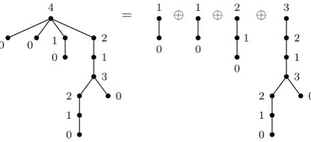
root(T) denote the root label of T, and let sub(T) denote the number of children of the root. We say that aβ(0,1)-treeT isreducibleif sub(T)>1, andirreducible
otherwise. Any reducible tree can be written as a sum of irreducible ones, where the sum U⊕V of two treesU andV is defined as the tree obtained by identifying the roots ofU andV into a new root with label root(U)+root(V)−1. See Figure 2, taken from [1], for an example.
4
0 0 1 2
[image:4.595.183.411.359.463.2]0 1 3 2 1 0 0 = 1 0 ⊕ 1 0 ⊕ 2 1 0 ⊕ 3 2 1 3 2 1 0 0
Figure 2. Decomposing a reducibleβ(0,1)-tree.
Note also that any irreducible tree with at least one edge is of the form λi(T), where 0≤i≤root(T) and λi(T) is obtained from T by joining a new root via an edge to the old root; the old root is given the labeli, and the new root is given the label i+ 1. For instance,
if T = 2
0 1
0
then λ0(T) = 1 0
0 1
0
, λ1(T) = 2 1
0 1
0
, and λ2(T) = 3 2
0 1
0 .
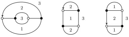
The smallest bicubic map has two vertices and three edges joining them. It is known [3] that the faces of a bicubic map can be colored using three colors so that adjacent faces have distinct colors, say, colors 1, 2 and 3, in a counterclockwise order around white vertices. We will assume that the root vertex is black and the root face has color 3. There are exactly three different bicubic maps with 6 edges and they are given in Figure 3 appearing in [1].
1 3 2
3
2 1 2
3
1 2 1
[image:5.595.184.408.122.186.2]3
Figure 3. All bicubic maps with 4 vertices.
the 1-colored face that meets the vertex that the root edge points to:
R1 R2 S1
R3
We say that a face touches another face ktimes if there arek different edges each belonging to the boundaries of both faces. Define the following two statistics:
f1r3(M) is the number of faces inF1(M) that touchR3;
s1r3(M) is the number of timesS1 touchesR3.
We say that M is irreducibleif s1r3(M) = 1, or, in other words, if S1 touchesR3 exactly once; we say that M isreducible otherwise. We shall introduce operations on bicubic maps that correspond toλi and⊕ofβ(0,1)-trees. This will induce the desired bijectionψ between bicubic maps andβ(0,1)-trees.
To construct an irreducible bicubic map based on M, and having two more vertices than M, we proceed in one of two ways. The first way (1) corresponds to λi(T) wheni = root(T); the second way (2) corresponds to λi(T) when 0 ≤i < root(T).
(1) We create a new 1-colored face touching the root face exactly once, so f1r3(M0) = f1r3(M) + 1, by removing the root edge fromM and adding a digon that we connect to the map as in Figure 4.
M
3 7−→ M0 = M
1 2
[image:5.595.213.379.494.554.2]3
Figure 4. Creating an irreducible map.
(2) Assuming that f1r3(M) = k; that is, M hask (different) 1-colored faces touching the root face, we can create an irreducible map M0 such that f1r3(M0) =i, where 1≤i≤k. To this end, we remove the root edge from M. Starting at the root vertex and counting inclockwise direction, we also remove the first edge of theith 1-colored face that touches the root face. In the picture below we schematically illustrate the case i= 3. Next we add two more vertices and respective edges, and assign a new root as shown in Figure 5.
Any irreducible bicubic map onn+ 2 vertices can be constructed from some bicubic map onnvertices by applying operation (1) or (2) above.
M
3
1 1
1 1
7−→ M0 = M
3
3
2 1 1
[image:6.595.174.418.142.212.2]1 1
Figure 5. The other way to create an irreducible map.
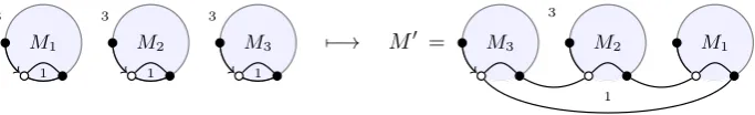
(3) We begin by lining up the mapsM1, M2, . . . ,Mk. Next, in each mapMi, we remove the first edge (incounter-clockwise direction) from the root edge on the root face. Then we connect the maps as shown in Figure 6, and define the root edge of the obtained map to be the root edge ofMk.
1
M1 3
1
M2 3
1
M3 3
7−→ M0 = M3 M2
1
M1 3
Figure 6. Creating a reducible map.
Any reducible bicubic map on n vertices can be constructed by applying the above operation (3) to some ordered list of irreducible bicubic maps whose total number of vertices isn.
By defining operations on bicubic maps corresponding to the operations λi and
⊕ we have now completed the definition of the bijectionψ between bicubic maps and β(0,1)-trees. See [1] for examples of non-trivial applications of the bijection.
3. Gray codes
In this section, after introducing some notations, we will define a Gray code for β(0,1)-trees with the same underlying tree and extend it to a cyclic Gray code for β(0,1)-trees with arbitrary underlying trees. This will induce a cyclic Gray code for bicubic maps. Then we will see that our construction can be easily extended to a wider class ofβ-description trees inducing cyclic Gray codes for the corresponding planar maps.
A listL for a set of lengthntuples is aGray codeifLlists, with no repetitions nor omissions, the tuples in the set so that the Hamming distance between two successive tuples inL(i.e., the number of positions in which they differ) is bounded by a constant, independent of n. And when we want to explicitly refer to this constant, sayk, we call such a list a k-Gray code. In addition, if the last and first tuple inLdiffer in the same way, then the Gray code is cyclic.
IfLis a list, thenLis the list obtained by reversingL, and ifMis another list, then L ◦ Mis the concatenation of the two lists. Ifαis a tuple, then α· L(resp.,
[image:6.595.130.472.332.384.2]Given a family {L1,L2, . . . ,Lm} of m lists, each Li, 1 ≤ i ≤ m, being a ki -Gray code for a set Li of same length tuples, we define another family of lists
{N1,N2, . . . ,Nm} as follows: N1 is simply the listLm, and for 2≤i≤m,
Ni=e1· Ni−1◦e2· Ni−1◦e3· Ni−1. . . ,
where he1, e2, e3, . . . , ejiis the listLm−i+1, and the last term of the concatenation defining Ni is either ej· Ni−1 orej· Ni−1, depending onj being odd or even.
It is routine to prove the following proposition that we will use later.
Proposition 1. With the notations above, Nm is a k-Gray code for the product
set L1×L2× · · · ×Lm, wherek= max{k1, k2, . . . , km}.
3.1. Gray coding β(0,1)-trees with the same underlying tree. Recall that by definition, the label of the root of a β(0,1)-tree is uniquely determined by the labels of its children. In what follows, for convenience, we assume that the root of any β(0,1)-tree is labeled by∗. That is, we amend (2) in Definition 2, obtaining a class of trees, still calledβ(0,1)-trees by us, which are in one-to-one correspondence with β(0,1)-trees defined either in Definition 1 or Definition 2. The rationale for (again!) updating slightly our previous definitions is in allowingβ(0,1)-trees to be of distance 1 from each other in the sense specified in Definition 6 below.
We are also interested in the following class of labeled trees, which are essentially β(0,1)-trees, but where the root is treated as any other internal vertex.
Definition 3. Aβ0(0,1)-tree is a rooted plane tree whose vertices are labeled with nonnegative integers such that
(1) leaves have label 0;
(2) the label of any other vertex exceeds the sum of its children’s labels by at most 1.
Note that anyβ(0,1)-tree discussed in Definition 2 is aβ0(0,1)-tree.
Definition 4. Let T be a β(0,1)-tree or a β0(0,1)-tree. Then u(T) denotes the underlying rooted tree, that is, the tree obtained by removing all labels in T. In other words, u(T) gives the shape ofT.
For example, if T is the rightmost β(0,1)-tree in the top row in Figure 1, then u(T) is given by
Definition 5. Let T be a β(0,1)-tree or a β0(0,1)-tree with n vertices. We let `(T) denote then-tuple ofT’s labels obtained by traversingT by depth first search using the leftmost option and reading each label exactly once.
For example, for the tree T in Figure 2,`(T) = (4,0,0,1,0,2,1,3,2,1,0,0); see also Table 2 where the roots are labeled by *. Thus,`(T) is an encoding of a given β(0,1)-treeT in the form of a tuple. Note that this encoding disregards the shape of the tree.
For example, keeping in mind that we label the root of a β(0,1)-tree by∗, the distance between the first and the fourth trees in the top row in Figure 1 is 2, while the distance between the first and the second trees in the bottom row in that figure is 1.
Definition 7. For a β0(0,1)-treeT, we letL(T) denote the set of encodings of all β0(0,1)-trees obtained by labeling properlyu(T).
Lemma 2. For any β0(0,1)-tree T there is a1-Gray code for L(T).
Before giving a formal proof of Lemma 2, we explain its general idea, which is presented graphically in Figure 7(a). Assuming the existence of a 1-Gray code for smaller trees, we can extend such a code to trees obtained by adding the new root. More precisely, each vertex in Figure 7(a) corresponds to a β0(0,1)-tree having a fixed shape (that is, underlying tree). Vertices on the same vertical line correspond to β0(0,1)-trees that differ only in the root label: the higher a vertex is, the larger root label it corresponds to. Note that each vertical line must contain at least the vertices corresponding to root labels 0 and 1, but it may or may not contain other vertices.
Further,a1,a2, etc. in this figure form a Hamiltonian path corresponding to the 1-Gray code for the trees with root label equal to 0, whose existence we assumed. Also, b1,b2, etc. is such a path for the trees with root label equal to 1. Thus, the trees corresponding toaiandbidiffer only in the root label. The desired Hamilton-ian path through all theβ0(0,1)-trees (corresponding to the 1-Gray code forL(T)) presented schematically in Figure 7(a) begins ata1and goes in the direction of the arrow.
Proof of Lemma 2. We proceed by induction on the number v of vertices in T. The base cases, v = 1 (the single vertex β0(0,1)-tree) andv = 2 (two single edge β0(0,1)-trees, which are on distance 1 from each other) obviously hold.
Suppose now that v ≥3, and the children of the root are the roots of subtrees T1, T2, . . . , Tk from left to right, where k ≥ 1. Each Ti is a β0(0,1)-tree and by induction hypothesis, L(Ti) has a 1-Gray code. But then, by Proposition 1,
L(T1)×L(T2)× · · · ×L(Tk)
also has a 1-Gray code, and it can be extended to a 1-Gray code ofL(T) obtained by adding the new leftmost coordinate corresponding to T’s root to each entry of L(T1)×L(T2)× · · · ×L(Tk) as explained below.
For an integeru≥0 we define two lists of 1-tuples:
• γ(u) =h(0),(u),(u−1), . . . ,(2),(1)i, and
• δ(u) =h(1),(u),(u−1), . . . ,(2),(0)i.
In particular,γ(1) andδ(1) are the listsh(0),(1)iandh(1),(0)i, respectively. Lethα1, α2, . . .ibe the 1-Gray code list forL(T1)×L(T2)× · · · ×L(Tk), so that eachαj is the concatenation ofktuples corresponding to the labels of the vertices of the trees T1, T2, . . . , Tk, and let m(αj) be the sum of the labels of the roots of these trees plus one. In other words, m(αj) is the maximal value ofx, such that (x)·αjis a proper labeling ofT. Thusm(αj)≥1 andm(αj) = 1 if and only if the root of eachTi is labeled by 0. Finally, letMbe the list defined as
M=M1◦ M2◦ M3◦ · · ·
with
Mj=
(a) (b)
Figure 7. Schematic approach in the proof of (a) Lemma 2, and (b) Lemma 6.
Clearly, the underlying set of M is L(T). In addition M is a 1-Gray code: throughout each list Mj successive tuples differ in the first position, and the last element ofMj differ from the first element ofMj+1asαjdiffer fromαj+1, that is in a single position.
Thus,L(T) has a 1-Gray code and the statement is proved by induction.
Theorem 3. There exists a 1-Gray code forβ(0,1)-trees having the same under-lying tree.
Proof. Suppose that the root of aβ(0,1)-treeT, labeled by∗, has subtreesT1, . . . , Tk, where k ≥1. Each Ti is a β0(0,1)-tree, and thus, by Lemma 2, there is a 1-Gray code for each L(Ti). But then, by Proposition 1, there is also a 1-Gray code for L(T1)×L(T2)× · · · ×L(Tk) leading to the fact thatL(T) ={(∗)} ×L(T1)×L(T2)×
· · · ×L(Tk) has a 1-Gray code, as desired.
Note that generally speaking the 1-Gray codes in Lemma 2 and Theorem 3 are not cyclic, and below we discuss how cyclic 1-Gray codes in this context can be obtained.
3.2. Gray coding cycliclyβ(0,1)-trees with the same underlying tree. The results presented in the previous subsection can be generalized to cyclic Gray codes in question. The goal of this subsection is to justify this, and in contrast with the previous subsection, here the proofs will be rather existential than constructive. First note that Proposition 1 can be generalized to the following proposition that is easy to prove directly, but also it follows from more general results presented in [4].
Proposition 4. Suppose thatL1, L2, . . . , Lmare sets, and each of them is a set of
same length tuples which is either a singleton, or there is a cyclic 1-Gray code for it. Then there is a cyclic1-Gray code for the product setL1×L2× · · · ×Lm.
In what follows we will need the following easy to understand facts.
Fact 5. Let G be a1-Gray code for a set of lengthk tuples.
• If r = (r1, . . . , rk) and s = (s1, . . . , sk) are consecutive tuples in G, then
there are noi andj,1≤i6=j ≤k, such thatri6=si andrj6=sj.
• If t = (t1, . . . , tk) is a third tuple, and r, s andt are consecutive (in this
order) in G and there is an i withsi∈ {/ ri, ti}, thenri6=ti.
Indeed, in this case the first and the last vertices in P area1 and am, wheremis the maximum index, anda1 andamare connected by an edge.
Thus, the difficult case is when the number of ais is odd, which is possible (e.g. there are fiveβ0(0,1)-trees having the shape of a path on three vertices). To handle this situation, we use the idea presented in Figure 7(b). Namely, we will prove that essentially in all cases, there is an edgec1c2between twoβ0(0,1)-trees having root label 2 such that the edges corresponding to it on levels “root label = 0” and “root label = 1” are involved in the respective Hamiltonian cycles assumed by the induction hypothesis (these edges are akak+1 andbkbk+1 in Figure 7(b)). The existence of c1c2 allows us to change the turns taken from the two Hamiltonian cycles making sure that the first and the last vertices in P will be a1 andam. In what follows, for a given tree we will refer to a vertex different from the root or a leaf as internal vertex. The two situations when c1c2 does not exist are easy to handle. This happens when
• there are no internal vertices in a tree. For a given number of vertices, there are only two such β0(0,1)-trees, any listing of which gives a cyclic 1-Gray code;
• there is exactly one internal vertex in a tree. One can easily check that, for any treeT with exactly one internal vertex, there are fiveβ0(0,1)-trees with the shape ofT, and the number of such trees with root label 0 (equivalently, 1), which is the number of ai’s (equivalently,bi’s) is two, which is even, so that the existence of a Hamiltonian cycle in this case is easy to establish using the approach in Figure 7(a). For example, the (ordered) list below is a cyclic 1-Gray code for theβ0(0,1)-trees of same shape on four vertices:
0 0
0 0
0 0
0 1
0 0
1 1
0 0
1 2
0 0
1 0
Recall from Definition 7 that for aβ0(0,1)-treeT,L(T) denotes the set of encod-ings of all β0(0,1)-trees obtained by labeling properlyu(T). The following lemma generalizes Lemma 2.
Lemma 6. For any β0(0,1)-tree T there is a cyclic1-Gray code for L(T). Proof. Based on the discussion preceding the statement of this lemma, the proof of Lemma 2 can be used if we will prove the existence of an edgec1c2 in the situation when T has at least two internal vertices. If the subtrees of T are T1, T2. . . , Tk, the existence of c1c2 is equivalent with the existence of two successive tuples in the Gray code for the product setL(T1)×L(T2)× · · · ×L(Tk) which both can be extended to proper labeling of T by letting the root of T be 2. To this end, we consider two subcases.
• The root ofThas exactly one internal vertexvamong its children. It follows that, Tj, the subtree rooted in v in turn has at least one internal vertex among its children. It is easily seen that the product setL(T1)×L(T2)×
the successor and the predecessor of u, in the Gray code forL(Tj), has a non-zero value in the position corresponding tov, the root ofTj. It follows that there are two successive tuples in the Gray code forL(Tj), and so for the above product set, which can be extended to a proper labeling ofT by letting the root of T be 2, which is allowed by the rules of β0(0,1)-trees; and this extension will give us the desired edgec1c2.
• The root of T has at least two internal vertices among its children. Let i andjbe the positions corresponding to the labels of two of these vertices in the tuples inL(T1)×L(T2)× · · · ×L(Tk). Clearly, 1 is an admissible value for the entries in positions i and j. Let ube a tuple in L(T1)×L(T2)× · · · ×L(Tk) having 1 in both positionsiandj. By the first point of Fact 5 it follows that if uis not the last tuple in the Gray code for the product set L(T1)×L(T2)× · · · ×L(Tk) (whose existence we assume by inductive hypothesis and Proposition 4), then the successor ofuhas 1 in at least one of these two positions. The reasoning is similar when u is the last tuple by replacing “successor” by “predecessor”. And again, it follows that there are two successive tuples in the Gray code for L(T1)×L(T2)× · · · ×L(Tk) which can be extended to proper labeling of T by letting the label of the root ofT be 2.
Thus, in both cases there is a 1-Gray code for L(T) with the first and last tuple of the form (0, α1, α2, . . .) and (0, ω1, ω2, . . .), respectively, where(α1, α2, . . .) and (ω1, ω2, . . .) are the first and last tuples in the cyclic Gray code for the product set L(T1)×L(T2)× · · · ×L(Tk), and the statement follows.
Using Lemma 6, we can now generalize Theorem 3, which is the main result in this subsection.
Theorem 7. There exists a cyclic 1-Gray code for β(0,1)-trees having the same underlying tree.
Proof. Suppose that the root of aβ(0,1)-treeT, labeled by∗, has subtreesT1, . . . , Tk, where k ≥ 1. Each Ti is a β0(0,1)-tree, and thus, by Lemma 6, there is a cyclic 1-Gray code for each L(Ti). But then, by Proposition 4, there is also a cyclic 1-Gray code for L(T1)×L(T2)× · · · ×L(Tk) leading to the fact that L(T) ={(∗)} ×L(T1)×L(T2)× · · · ×L(Tk) has a cyclic 1-Gray code, as desired.
Since the tuple (∗,0,0, . . . ,0) of appropriate length is always an admissible en-coding of a β(0,1)-trees, we have:
Corollary 8. There exists a 1-Gray code list for β(0,1)-trees having the same underlying tree which begins by (∗,0,0, . . . ,0) and ends by a tuple differing from
(∗,0,0, . . . ,0) in exactly one position.
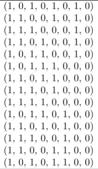
3.3. Dyck words and Gray coding bicubic maps. For two integerskandm, 0≤k≤m, we denote byDm,kthe set of binary tuples withmoccurrences of 1 and k occurrences of 0, satisfying the prefix property: no prefix contains more 0s than 1s. For example, (1,0,1,1,0,1,1,0,0)∈D5,4. The setDm,m is known as the set of
Dyck wordsof length 2m. The number of elements inDm,mis the well knownmth
(1, 0, 1, 0, 1, 0, 1, 0) (1, 1, 0, 0, 1, 0, 1, 0) (1, 1, 1, 0, 0, 0, 1, 0) (1, 1, 0, 1, 0, 0, 1, 0) (1, 0, 1, 1, 0, 0, 1, 0) (1, 0, 1, 1, 1, 0, 0, 0) (1, 1, 0, 1, 1, 0, 0, 0) (1, 1, 1, 0, 1, 0, 0, 0) (1, 1, 1, 1, 0, 0, 0, 0) (1, 0, 1, 1, 0, 1, 0, 0) (1, 1, 0, 1, 0, 1, 0, 0) (1, 1, 1, 0, 0, 1, 0, 0) (1, 1, 0, 0, 1, 1, 0, 0) (1, 0, 1, 0, 1, 1, 0, 0)
Table 1. The Gray code listD4,4 for the set of length 8 Dyck words.
Note that the Hamming distance between two same length Dyck words is always even, and thus the minimum distance between two Dyck words is 2.
The following recursive description obtained in [11] gives a Gray code forDm,k, and, in particular, for the set of length 2mDyck words; this description is a slight variation of the code defined in [8]:
Dm,k=
(1)m if k= 0,
Dm,k−1·(0) if m=k >0,
Dm−1,k·(1)◦ Dm,k−1·(0) if m > k >0.
(1)
See Table 1, showingD4,4, for an example. The following lemma was proved in [11].
Lemma 9. [11] The listDm,k satisfies the following properties:
• The first tuple in Dm,kis (1,0)k·(1)m−k;
• The last tuple in Dm,k is
– (1,0)m−2·(1,1,0,0), if k=m >1,
– (1,0)k−1·(1)m−k+1·(0), ifm > k≥1 orm=k= 1,
– (1)m, if m > k= 0;
• Two successive tuples in Dm,k, including the last and the first one, differ
in exactly two positions, and thusDm,k is a cyclic2-Gray code.
In what follows, the Hamming distance between tuples is denoted byd, and the next definition extends it to trees.
Definition 8. For β(0,1)-trees T1 and T2 on the same number of vertices, the
distance d(T1, T2) between the trees is defined as
d(T1, T2) =d(`(T1), `(T2)) +d(w(u(T1)), w(u(T2))).
Theorem 10. There exists a cyclic 3-Gray code for β(0,1)-trees (with the root labeled by *)onnvertices, n≥1, with respect to the distance given in Definition 8.
Proof. Anyβ(0,1)-tree T onnvertices can be encoded by a (3n−2)-tuple, which is obtained by merging the (2n−2)-tuples w(u(T)) and then-tuples`(T). Let
d1· L(T(d1))◦d2· L(T(d2))◦d3· L(T(d3))◦ · · · (2)
It is easy to see that in the list defined in relation (2) two successive tuples are at distance at most 3. Indeed,
• for a fixed di, successive tuples indi· L(T(di)) differ in one position, and
• for two successive tuplesdianddi+1inDn−1,n−1(including the last and the first ones), the last tuple indi·L(T(di)) and the first one indi+1·L(T(di+1)) differ in three positions.
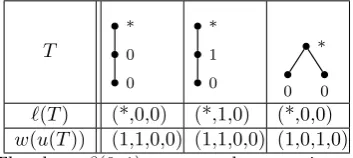
Note that the Gray code stated in Theorem 10 forβ(0,1)-trees is minimal, in the sense that, in general there are no cyclic 2-Gray codes forβ(0,1)-trees. See Table 2 for an example where β(0,1)-trees, encoded by (1,1,0,0,*,0,0), (1,1,0,0,*,1,0) and (1,0,1,0,*,0,0), cannot be listed cyclically so that the distance between successive trees is at most 2. Also, the Gray code defined in (2) is “shape partitioned”, that is, same shapeβ(0,1)-trees are successive in it.
T
0 0 *
0 1 *
0 0
*
[image:13.595.209.386.292.371.2]`(T) (*,0,0) (*,1,0) (*,0,0) w(u(T)) (1,1,0,0) (1,1,0,0) (1,0,1,0)
Table 2. The threeβ(0,1)-trees on three vertices with the root
labeled by *, and the corresponding to them the depth first leftmost option reading of the labels, and the Dyck words coding their shape.
Our way to Gray code bicubic maps can be applied to any class of planar maps that can be described in terms ofβ(a, b)-trees withb≥1. Namely, generalizing the notion of β0(0,1)-trees to that ofβ0(a, b)-trees (by removing the condition on the root in Definition 1), we can essentially copy/paste all our arguments for β0(0, 1)-trees. Indeed, for such a β0(a, b)-tree T, the levels corresponding to the root’s label aanda+ 1 will be isomorphic, so that induction can be used in the way we used it for β0(0,1)-trees. Thus, in particular, we can Gray code 3-connected cubic planar maps and cubic non-separable planar maps corresponding to β(1,1)-trees and β(2,2)-trees, respectively [2, 3].
Finally, note that havingb≥2 would simplify some of our arguments. In partic-ular, in this case there is no need to prove the existence of the edgec1c2in Lemma 6, since we will have at least three isomorphic levels of vertices corresponding to the root labelsa,a+ 1 anda+ 2, so that existence of an edge with the right properties will be given to us automatically (in fact, each edge from the Hamiltonian path on level a+ 2 will have the right properties).
4. Concluding remarks
In this paper we have shown that classes of planar maps corresponding toβ(a, b )-trees withb≥1 have cyclic 3-Gray codes, and these codes are minimal in the sense of Hamming distance. We leave it as an open problem to determine whether there exist (cyclic)k-Gray codes, for somek≥1, forβ(a,0)-trees, wherea≥1. In the case a= 1 such a code would induce a Gray code on non-separable planar maps via the respective bijection [2].
Acknowledgments
The authors are grateful to the anonymous referee for reading carefully the man-uscript and for providing many useful suggestions, in particular, on a proper in-troduction of maps. The first and the third authors were supported by Grant NSh-1939.2014.1 of President of Russia for Leading Scientific Schools. The sec-ond author is grateful to Lsec-ondon Mathematical Society and to the University of Bourgogne for supporting his work on this paper.
References
[1] A. Claesson, S. Kitaev and A. de Mier. An involution on bicubic maps and beta(0,1)-trees, Australasian J. Combin.61(1)(2015) 1–18.
[2] R. Cori, B. Jacquard and G. Schaeffer. Description trees for some families of planar maps, Formal Power Series and Algebraic Combinatorics(1997) 196–208. Proceedings of the 9th Conference, Vienna.
[3] R. Cori and G. Schaeffer. Description trees and Tutte formulas,Theoret. Comput. Sci.292
(1997), 165–183.
[4] V. V. Dimakopoulos, L. Palios and A. S. Poulakidas. On the Hamiltonicity of the Cartesian product.Inform. Process. Lett.96(2005), no. 2, 49–53.
[5] R. W. Doran. The Gray code,J.UCS13(11)(2007) 1573–1597.
[6] W. M. B. Dukes, M. F. Flanagan, T. Mansour and V. Vajnovszki. Combinatorial Gray codes for classes of pattern avoiding permutations.Theoretical Computer Science396(2008) 35–49. [7] S. Kitaev. Patterns in permutations and words, Springer-Verlag, 2011.
[8] F. Ruskey and A. Proskurowski. Generating binary trees by transpositions,Journal of Algo-rithms11(1990) 68–84.
[9] F. Ruskey. Combinatorial gseneration, book in preparation.
[10] C. Savage. A survey of combinatorial Gray codes,SIAM Rev.39(4)(2006) 605–629. [11] V. Vajnovszki, Generating a Gray code forP–sequences,IJMA1(2002) 31–41. [12] W. T. Tutte. A census of planar maps,Canad. J. Math.67(1963) 15, 249–271.
[13] W. T. Tutte.Graph Theory As I Have Known It, Oxford University Press, New York, 1998. [14] T. Walsh. Generating Gray Codes in O(1) worst-case time per word,4thDiscrete Mathe-matics and Theoretical Computer Science Conference, Dijon-France, 7–12 July 2003 (LNCS, 2731, 73–88).
Sobolev Institute of Mathematics, 4 Acad. Koptyug Ave, 630090 Novosibirsk, Russia, [email protected]
Department of Computer and Information Sciences, University of Strathclyde, 26 Richmond Street, Glasgow G1 1XH, United Kingdom,[email protected]
Sobolev Institute of Mathematics, 4 Acad. Koptyug Ave, 630090 Novosibirsk, Russia, [email protected]