An efficient order reduction strategy in earthquake nonlinear response analysis of structures

Crete Island, Greece, 5–10 June 2016

AN EFFICIENT ORDER REDUCTION STRATEGY IN EARTHQUAKE

NONLINEAR RESPONSE ANALYSIS OF STRUCTURES

F. Bamer1_{, A. Kazemi Amiri}2_{and C. Bucher}3

1 _{RWTH-Aachen University, Institute of General Mechanics,} Templergraben 64, 52062 Aachen, Germany

e-mail: [email protected]

2_{Vienna Doctoral Programme on Water Resource Systems,} TU Vienna, Karlsplatz 13/222, 1040 Vienna, Austria

e-mail: mehrad [email protected]

3_{Center for Mechanics and Structural Dynamics,} TU Vienna, Karlsplatz 13/206, 1040 Vienna, Austria

e-mail: [email protected]

Keywords: Model order reduction, Proper orthogonal decomposition, Friction pendulum sys-tem

1 INTRODUCTION

The evaluation of the response history of a structure in the time domain is one of the main topics in earthquake engineering and structural dynamics. Often it is common practice to create simple structural models, e.g. multistory shear frames, which should be able to describe the structural behavior and peculiarities of the real structure. This approach leads to useful results for the investigation of rather simple and uniform structures in order to draw meaningful engi-neering decisions regarding structural resistance. On the contrary, the analysis of complicated systems can require the application of nonlinear high-order systems, as a characterization by a low dimensional structural model could lead to an oversimplification, i.e. important motion patterns could be ignored. Therefore, an effective strategy is to obtain a set of a low number of “important” equations of motion that approximates the high-dimensional nonlinear dynamical system as accurately as possible, that is, model order reduction (MOR).

The solution of the nonlinear set of equations of motion in the time domain is realized by numerical algorithms, which require computational effort if the number of DOF is high. Even the response calculation of linear systems can be expensive, as a factorization of the stiffness matrix is necessary to solve the eigenvalue problem and calculate the natural modes of vibration. An alternative is to replace a high-dimensional nonlinear set of equations of motion by a reduced set, providing the main dynamic behavior of the system to reach the required level of accuracy. MOR methods are used in many fields of research, where high-dimensional systems are dealt. Some review papers of MOR, especially for structural dynamic applications, are presented by Rega and Troga [3] and Koutsovasilis and Beitelschmidt [4] as well as the books of Qu [2] and Schilders et al. [5]. The classical but also effective method of modal truncation is well-known in the field of earthquake engineering, which is however mainly applicable to linear systems.

This paper concentrates on a new MOR strategy based on the proper orthogonal decompo-sition (POD) method. The POD provides a low dimensional uncorrelated description (basis vectors), by which a high-dimensional correlated process, e.g. structural response, is spanned. Firstly, it was used as a statistical formulation in the papers of Kosambi [6], Karhunen [7] and Loeve [8]. Following this mathematical basis of the POD, which is also known as Karhunen-Loeve Decomposition and Principal Component Analysis, was applied in many fields of re-search, including turbulence and coherent structures, wind engineering, image processing and structural dynamics.

The first paper regarding the field of structural dynamics was written by Cusumano et al. [9] in the early 1990’s, who presented an experimental study of dimensionality in an elastic impact oscillator. In the papers [10] and [11] of Feeny and Kappagantu a relation of the proper orthogonal modes to normal modes of vibration is investigated. Then they used the POD as they so call optimal modal reduction and exploit the benefits of the application of these modes in comparison to the linear natural modes. Furthermore, Kappagantu and Feeny investigated in [12] and [13] the dynamics of an experimental frictionally excited beam and they verified that the proper orthogonal modes are efficient in capturing the dynamics of the system. Liang et. al. [14] discuss the realizations of the POD, i.e. Karhunen-Loeve Decomposition, principal component analysis and singular value decomposition and compare these three methods. Ker-schen and Golivani [15] analyze the physical interpretation of the POD modes and its relation to the singular value decomposition and in [16] they investigated POD based on auto-associative neural networks.

MOR, has aroused interests mainly in the last two decades in the field of earthquake engineer-ing, some papers related to this issue are e.g. [27] and [28]. More specified to the related issue Tubino et. al. [17] investigated the seismic ground motion of the support points of a structure and denominate the POD as a very efficient tool to simulate multi-variate processes. Bucher [32] examined the stabilization of explicit time integration methods for analysis of nonlinear structural dynamics by modal reduction. Gutierrez and Zaldivar investigated in [30] how to handle the stability problem of explicit time integration by modal truncation methods more re-lated to problems in earthquake engineering and structural dynamics and following in [29], they applied the Karhunen-Loeve Decomposition, which is formally identical to the POD analysis, to capture the essential characteristics of nonlinear systems and provide experimental examples conducted on a shaker table. Bamer and Bucher [18] developed a MOR strategy applying the POD method for transient excited structures resting on one-dimensional friction elements. This study presented a powerful combination of the POD and explicit time integration schemes.

The current work investigates the extension of the POD-based MOR strategy, which is ap-plicable to nonlinear systems in contrast to the method of modal truncation. The new strategy pursues the following objective: a low number of deterministic nonlinear modes (i.e. set of POD modes) is determined that defines a representative characterization of the structural be-havior. Therefore, due to the information content of the full or a part of the time response of the structure to one representative excitation a set of deterministic modes, i.e. POD modes, is evaluated. Subsequently, this set of modes is utilized to project the equations of motion of a structure under different earthquake excitations onto POD coordinates and following an order truncation is performed in a similar manner as the application of modal truncation to linear systems.

It is attached importance to demonstrate this new strategy and its advantages on a practical application. The method is applied to the dynamic model of a realistic building structure. The building is erected on friction pendulum bearings for the sake of seismic isolation to minimize the transferred acceleration to the building during an earthquake. A three-dimensional dynamic model of the base isolated structure is derived by implementing the finite element model of the structure and the bi-directional friction pendulum systems. The subsequent section deals with the nonlinear dynamic model of the base-isolated structure. Following, the new POD-based MOR strategy and the example of its practical application is provided. Finally, the discussion on the results and conclusions are given.

2 Nonlinear model order reduction

Then-dimensional set of equations of motion of a structure with nonlinear material behavior excited by horizontal components of ground acceleration is expressed as (cf. Chopra [20])

M¨x+C ˙x+R(x) =−M(fxx¨g+fyy¨g) , (1)

whereMandCare mass- and damping square matrices of ordern andR(x)is the nonlinear internal restoring force vector dependent on the displacement x with the dimension n × 1. The right hand side of the set of equations of motion describes the earthquake excitation term, whilex¨g andy¨g denote the ground acceleration inx- andy-direction andfj,(j =x, y) are the influence vectors in the corresponding direction. It is

fx(xi) = 1, fy(yi) = 1 , i= 1...n , (2)

at the globalxandydegrees of freedom of all nodes, whereas the other components offxand

approach indicates that in this paper the ground acceleration in the corresponding direction, i.e.

x-,y- orz-direction, is equal in all structural support points. In the following equations the term on the right hand side of the set of equations of motion (1) is denominated byF(t), which has the unit of a force.

Nonlinear systems, as they are depicted in Equation (1), have generally to be solved by the application of a numerical algorithm, that is, a step by step procedure in the time domain in order to obtain the response of the structure as a function of time. The necessity of application of a numerical method inevitably leads to the existence of computational effort if n is a large number. Therefore, the approximation by a low, dimensional description of the system seems to be useful, i.e. the application of MOR.

The main goal of MOR techniques is primarily to define a transformation matrix T ∈ Rn×m, m n to approximate the displacement vector x ∈ Rn through a reduced

coordi-nate vectorqr ∈Rmby the relation (cf. Koutsovasilis and Beitelschmidt [19])

x=Tqr , (3)

such that the dynamic properties of the system are preserved and the error is small. The notation of the variablem∈_Nis the dimension of the reduced subspace.

The projection of the nonlinear system defined by Equation (1) onto that subspace leads to another second-order ordinary differential equation (cf. Koutsovasilis and Beitelschmidt [19])

mr¨qr+crq˙r+r=fr, (4)

where mr = TTMT, cr = TTCT ∈ Rm×m are mass- and damping matrix and fr =

TTF(t) ∈ _Rm×1 _{is the force vector in the reduced subspace. It should be noted that the} re-duced system matricesmr andcrare generally not diagonal. The vector of the restoring forces in the reduced subspace is

r=TTR(x) = TTR(Tqr). (5)

Consequently, one necessity of nonlinear MOR is the evaluation of the vector of the restoring forces in the physical (full) coordinate at every time step.

3 The proper orthogonal decomposition and nonlinear modes

Modal truncation is a widely-used tool and an effective method for order reduction of linear systems in the field of earthquake engineering. An accurate approximation of the response history is achieved by applying a small number of lower structural modes proportional to the number of degrees of freedom. In this work, the objective is to find a new strategy that is applicable to nonlinear systems in a similar manner to modal truncation. The approach is to define a set of deterministic modes that can be evaluated from the information of an existing response history of the structure. Consequently, this set of modes contains nonlinear motion patterns if the structure shows nonlinear response behavior to the excitation.

The aim of the POD is to find a set of ordered orthonormal basis vectors in a subspace so that samples in a sample space are expanded in terms oflbasis vectors in an optimal form. This means that the POD is able to find an orthonormal basis, which describes an observation vector in a subspace better than any other orthonormal basis can do. A measure for this problem is the mean square error (cf. Qu [2])

Ekx−x(l)k2 ≤Ekx−ˆx(l)k2 , (6)

wherex ∈ _Rn×1

is the random vector, x(l)is the approximation of this random vector in an

l-dimensional POD subspace andˆx(l)is the approximation of the random vector by any other possible orthonormal basis. Therefore, the random vector can be expressed as (cf. Qu [2])

x=Φpqp, Φp = [ϕp,1, ϕp,2, ..., ϕp,s] and qp = [qp,1, qp,2, ..., qp,s], (7)

where ϕp,i are the POD modes and qp,i denote the coordinates in the POD subspace and s is the number of realizations of the random vector (also called snapshots). This leads to an optimization problem with the following objective function (cf. Qu [2])

2(l, t) =E

kx−x(l)k2 _→min

(8)

subject to the orthonormality condition (cf. Qu [2])

ϕT_p,iϕp,j =δij (i, j = 1,2, ..., s). (9)

The transformation into thel-dimensional POD subspace is a truncation of the firstllower POD modes (cf. Qu [2])

x(l)≈Φpqp , Φp= [ϕp,1, ϕp,2, ..., ϕp,l], l < sn . (10)

In structural dynamics, systems are discretized in space and time and the random vector is realized bysobservations at different time instances (cf. Han and Feeny [25])

Xs = [xt1,xt2, ...,xts] =





x1(t1) · · · x1(ts)

· · · · xn(t1) · · · xn(ts)



 . (11)

These observation vectors xti are called snapshots and, therefore, in the literature often the

observation matrixXsis called snapshot matrix containingssnapshots (observations). xtican

be measurements or solution vectors of a dynamical system at different time instances ([21]). Ifµis the expectation of all observations, then the sample covariance matrixΣsof this random vector, which is realized by the observation matrix, is defined by (cf. Kerschen et. al. [26])

Σs=E{(x−µ)T(x−µ)}. (12)

The POD modes and the POD values are defined by the eigensolution of the sample covariance matrix. If the data have zero mean, the covariance matrix is (cf. Kerschen et al. [26])

Σs=

1 sXs

T_X

s (13)

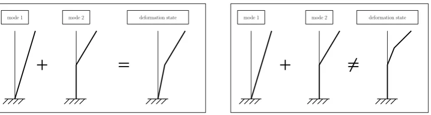
mode 1 mode 2 deformation state

Figure 1: Appropriate mode superposition

mode 1 mode 2 deformation state

Figure 2: Inappropriate mode superposition

the singular values ofXs, which are all real and positive and arranged in a rectangular diagonal matrix in descending order. The energy, which is contained by the snapshot matrix, is defined by the summation of the POD values, i.e. V = Ps

i=0λp,i. As a consequence, the energy ratio of theithPOD mode is (cf. Kerschen et al. [26])

Vi =

λp,i

Ps i=0λp,i

. (14)

In structural dynamics applications the sum of only a few POD values often captures 99.99

percent of the total energy included in the observation matrix, which reflects the big advantage of the POD, i.e. the property of optimality with respect to energy in a least square sense.

Practically, nonlinear effects must be sufficiently captured in the snapshot matrix (11) de-rived from the representative earthquake exciStructurestation. This is in order to create the capability of providing the possible nonlinear responses that can appear in the response history of the structure excited by another earthquake event. Consequently, nonlinear effects that are not contained in the snapshot matrix, such as plastic hinges or nonlinear sliding of a friction iso-lator cannot be displayed in the system response. This issue is depicted qualitatively in Figures 1 and 2. Two fictitious deformation states of a simple surrogate model are shown. Obviously, the two deterministic modes in Figure 1 are sufficient in order to represent the deformation state of the model. On the contrary, the set of deterministic modes is insufficient to represent the deformation state in Figure 2 and, consequently, the existing set of modes must be expanded by an additional mode in order to ensure a representation of the correct deformation state. Related to this paper, the conclusion is to capture nonlinear structural reactions in the snapshot ma-trix in order to provide accurate approximations of the structural response excited by different earthquake events.

Structures

4 The new strategy

representative earthquake excitation

snapshotsXs,

POD modesΦP

excitation 1

excitation 2

excitation 3

excitation 4

response 1

response 2

response 3

response 4

n

umeric

in

tegration

in

x

n

umeric

in

tegration

in

qP

MOR

x

−

→

qP

Figure 3: Approach of the new strategy

the snapshot records in equidistant time instances over the whole time history of the earthquake response. Additionally, it is of highest advantage to evaluate the full solutions to more than one earthquake event and spread the snapshots over all of the response histories. This procedure increases the probability of capturing all necessary motion patterns in order to provide an accu-rate representation by the reduced set of equations. Different earthquake excitations can affect nonlinearities, such as plastic hinges, at different parts of the structure. However, the goal is to define as much nonlinear effects as possible in order to be prepared to assemble an adequate reduced order model of Structuresthe structure excited by new earthquake excitations.

The transformation matrix Φp, containing the POD modes is calculated from the snapshot matrix by applying the SVD algorithm. Afterwards the transformation into the reduced sub-space is performed in the same manner, if the classical method of modal truncation would be applied to a linear system. The low-order set of equations of motion is then

f

M¨qP+C ˙eq_P+Re =Fe , (15)

whereMf = ΦT_PMΦ_P and Ce = ΦT_PCΦ_P are mass- and stiffness matrices and Fe = Φ_PFis

the excitation vector in the POD reduced subspace. The reduced vector of the inner restoring forcesRe is still dependent on the displacement in the physical coordinatex,

e

R=ΦT_PR(ΦPqP) =ΦTPR(x). (16)

Consequently, the vector of the inner restoring forcesR(x)has to be evaluated from the physical model in the full-order coordinates in every calculation time step. Furthermore, the equations of motion in the reduced-order set are not decoupled and have to be solved numerically. Finally, after the time integration procedure is conducted, the solution vector qP dependent on time is transformed back into the physical coordinatex. A visualization of this approach is depicted in Figure 3.

perform the full time integration procedure to solve the equation of motion (1). On the contrary, the critical time step of the POD reduced system described in equation (15) is much larger and, therefore, the number of calculation time steps is much smaller, which requires a fraction of computational effort compared to full-order system. These numerical issues are discussed in a similar manner by Gutierrez and Zaldivar [30] applied to modal truncation. For the numeri-cal benefit of the combination of the POD with explicit numeric time integration, the reader is referred to Bamer and Bucher [18]. The second big advantage of the new strategy is that the actual time consuming process, which is the evaluation of the snapshot matrix, is only executed once at the beginning of the whole calculation procedure. This a priori assumption of nonlinear mode patterns makes sense if the excitations show physical “similarities”, which is the case in earthquake analysis, where a considerably small number of lower modes is mainly affected.

5 Practical application

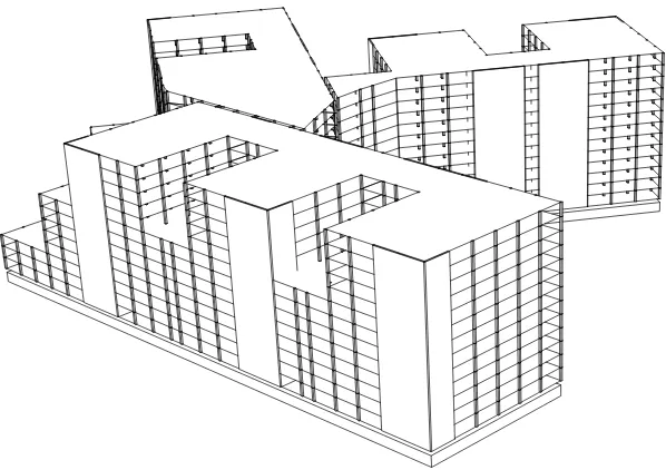
In addition to dealing with the development of the introduced POD-based MOR approach, it is within this section to represent the application of the new proposed MOR strategy on a realistic example. For this purpose, a dynamic structural model of a medical complex, according to its constructional plan, was derived. A schematic three-dimensional sketch of the building is depicted in Figure 4.

Figure 4: Three-dimensional visualization of the building construction

As shown in Figure 4, the building structure exhibits complex geometries. As a result, it seems to make sense to discretize the geometry by a finite element model in order to capture the main dynamic specifications.

are presented. Then, the displacement responses to a set of six earthquake events are evaluated. The numerical evaluations compare the new introduced strategy, as an alternative means, with the iterative Newmark integration scheme, which is known as an efficient and exact method.

5.1 Structural system and model specifications

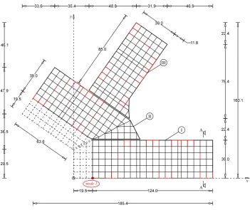
The building structure consists of three wings, referred to as wing I, II and III. Figure 5 shows a schematic sketch of the ground plan of the building containing the basic dimensions. The floor slabs of each wing are separate from the others except for the basement slab, which is indiscrete over all three wings. This means that all three wings are coupled through this slab and they work all together during earthquake excitations. However, the distance between the wings, which are connected by the basement slab, is about 1.5 meters, consequently, contact problems induced by ground motion are not considered in the computations.

The grid indicates the location of the columns and the binding beams, and the red lines indicate the location of the shear walls, which are responsible for the lateral reinforcement. The regular distance between the columns is 6.5 [m]. The building structure has three stories below the ground level, while the highest parts of the building above ground level have 13 stories and the remaining parts have eight stories including the basement levels. Therefore, the plan of the structure is irregular along its height along with the irregularities in the horizontal area. The dashed lines define the area, where the building is only located below the ground. The height of one story is three meters; this leads to a total construction height of42meters.

Below the three stories at the basement level, there is the indiscrete slab on the top of the isolators at level of −9.00 [m]. Below this slab, along each of the columns, a single friction pendulum (FP) bearing system is attached. Figure 6 depicts a part of the cross section A-A of the basement level shown in Figure 5. The horizontal diameter of the FP system is2.00meter. Thus, the dimension of the quadratic cross section of the columns in the basement and FP story is2.00×2.00 [m2_{], while in the remaining stories the columns are modeled as quadratic cross} sections with the dimensions 0.40×0.40 [m2_{]. All FP bearings have the same radius of the} concave surface, which is equal to3.00meters.

A representative full-scale finite element model of the building structure was created in the software package slangTNG [39]. The shear walls and slabs were modeled by shell/plate ele-ments and the columns and beams by beam eleele-ments. A linear elastic material was considered for the modeling purpose (Young’s modulusE = 3.5·1010 _[N

m2], Poisson’s ratioν = 0.3 [−],

densityρ = 2500 [_mkg3]). Nonlinear FP elements, whose implementation in slangTNG is

pre-sented in section 5.2, are assigned below the lowest basement plate of the structure. The total number of degrees of freedom is33000.

5.2 Dynamic model of the frictional pendulum element

Figure 5: Schematic ground plan, building construction (units in meters), output node1 [19.5,0.0,−9.5]T [m]

|U| ≈ √u2_+v2_{. The equivalent representation of such an element together with the acting} forces on it is represented in Figure 8.

The horizontal force equilibrium of the dynamical system is

FFr+Fk =Fex , (17)

whereFFr andFkare the elasto-plastic frictional- and centring force andFex = [Fx, Fy]T ac-counts for the interacting horizontal force, which couples the FP element to the super structure. Following, the force equilibrium is split into two parts as two dynamic situations can occur: situation stick and situation slide. The force equilibrium during the situation stick yields to

Fex =k1

u v

| {z }

Fk

+k2

∆u ∆v

| {z }

FFr

if |Fex−Fk|< µN . (18)

This relation renders a linearly-elastic system, where the friction coefficientµmust be a value between0and1(about0.04for a realistic implementation of the friction bearing) and the nor-mal contact force N acts orthogonal to the contact area of the slider and the concave surface. The vector ∆U = [∆u,∆v]T _{defines the radial distance with respect to the current sticking} point of the slider if the sticking condition is true.

During the situation slide the FP element is described by the following horizontal force equilib-rium

Fex =k1

u v

| {z }

Fk

+µN |U˙|

˙ u ˙ v

| {z }

FFr

if |Fex−Fk| ≥µN , (19)

whereU˙ = [ ˙u,v]˙ T _{is the velocity vector.}

In both relations, i.e. Eq. (18) and Eq. (19), the centring force|Fk|= k1r =k1

√

u2_+v2 _acts linearly orthogonal to the vertical axis through the deepest point of the surface and the center of the sphere. The fact that the centring force is linear indicates that the spherical shell of the real system is approximated by the paraboloid, whose potential energy increases with W_Rr in radial distance from the deepest point, i.e. the stiffness is inversely proportional to the radius of the spherek1 = W_R.

The frictional force FFr is modeled either linearly elastic or elastic-perfectly plastic as pre-sented in Eqs. (18) and (19), respectively. Note that the force corresponding to∆U accounts for the elastic behavior of the bearing coating material, in a small elastic range (situation stick, Eq. (18)) and acts towards the current location of the slider (not the center of the concave sphere). Generally, the implementation of a realistic model requiresk2 to be much larger than

U=(u,v,w)

x y

z

R

Figure 7: Geometric definitions of the FP element

Fk

FFr

slider (contact unit) W

Fx

Fy

Figure 8: Internal specifications of the FP element;Fx,

Fy,N, recentering forceFk, friction forceFF r

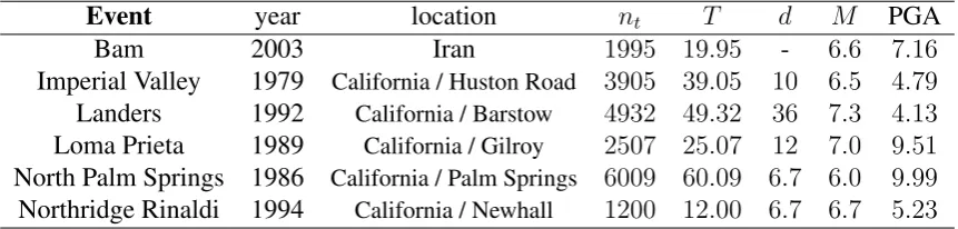
Event year location nt T d M PGA

Bam 2003 Iran 1995 19.95 - 6.6 7.16

Imperial Valley 1979 California / Huston Road 3905 39.05 10 6.5 4.79

Landers 1992 California / Barstow 4932 49.32 36 7.3 4.13

Loma Prieta 1989 California / Gilroy 2507 25.07 12 7.0 9.51

North Palm Springs 1986 California / Palm Springs 6009 60.09 6.7 6.0 9.99

Northridge Rinaldi 1994 California / Newhall 1200 12.00 6.7 6.7 5.23

Table 1: Earthquake excitation list;nt[−]number of time steps,T[s]duration of the record,d[km]distance from epicenter,M moment magnitude, PGA[m_/s2_{]peak ground acceleration}

to the weight of the structure. Considering the above-mentioned fact together with the force diagram given in in Figure 8, follows that the normal contact forceN is approximately constant and equal to the weight induced force of the super structure,W, i.e,N =W in Eq. (19).

The FP bearing element governed by Eqs. (17) to (19) has been implemented in the software package slangTNG [39]. For a comparable study on this implemented friction pendulum sys-tem, the experimental work of Mosqueda et al. [40] is suggested. For additional information about friction pendulum systems the reader is referred to the relevant literature (e.g. [33], [34], [35], [36], [37] and [38]). More detailed examination of this topic would lead beyond the scope of this paper, which should focus more on the methodical extension of the new MOR strategy as well as the application on a complex realistic system.

5.3 Numerical evaluation

inx- andy-direction are provided. The output node is called “node1” and has the coordinates

[19.5,0.0,−9.5]T [m], this is depicted in Figure 5. This node defines the location of a moving friction pendulum, it therefore shows directly the nonlinear response behavior of the system.

The method, according to Section 4, begins with the earthquake dynamic analysis of the structure under representative excitation. Therefore, the response XBam = [x1,x2, ...,xm]of the full system to the Bam earthquake is evaluated. This full system response is evaluated applying the Newmark method. The response history inx-direction of node1(output node) is depicted in the left subplot of Figure 9. The motion of the slider is shown in the right subplot of Figure 9.

0

20

-0.25

0

0.25

time [s]

x

[

m

]

-0.4

0

0.4

-0.4

0

0.4

x

[

m

]

y

[

m

]

Figure 9: Response functions to the Bam earthquake excitation, full Newmark response and reduced POD re-sponse; left subplot: displacementxof node1dependent on time; right subplot: movement of the slider, displace-mentxandyof node1

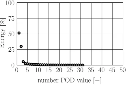
The snapshot matrix XS is assembled by taking into account 400 snapshots in equidistant time intervals spread over the whole displacement response history to the Bam earthquake ex-citation. It is essential to capture the main deformation behavior of the system in this stage, otherwise certain deformation states cannot be constituted by the set of linearly independent vectors (c.f. Figure 2), i.e. the sliding process, as can be seen in Figure 9, has to be recorded in the snapshot matrix. Afterwards, the evaluation of the left singular vectors of the snapshot matrix leads to the POD modes and its singular values to the POD values in descending order. The sum of all POD values define the total energy content of the snapshot matrix. Hence, the number of POD modes that have to be taken into account in order to capture99,99percent of the total energy was evaluated to be 31. A plot of the first 31singular values (POD values) dependent on the corresponding energy content is shown in Figure 10.

min-0 5 10 15 20 25 30 35 40 45 50 0

25 50 75 100

number POD value [−]

Energy

[%]

Figure 10: Number of POD values (singular values)

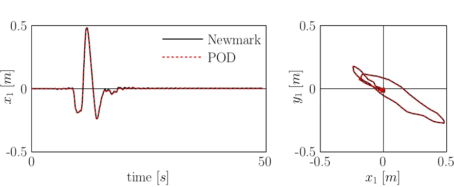
imum speed up factor of about2compared to the Newmark algorithm is achieved. However, it has to be added that for this type of nonlinearity, the Newmark integration scheme appears to have a relative slow convergence rate. As a consequence, the computational time by applying the Newmark method can exceed to a period of time, which is comparable if the full central difference integration scheme is applied or even to infinite period of time, if there is no conver-gence. Following, the new integration strategy gains the benefit of both of the two algorithms, i.e. central difference and Newmark, which is stability without requiring iteration algorithms. The red dashed line in Figure 9 (response to the Bam excitation) shows the response obtained by the new POD strategy, which approximates the full Newmark response accurately. This is not surprising as the snapshots are taken in equidistant time intervals spread over this whole response history. The derived POD transformation matrix, which is the set of POD modes, is now applied to reduce the order of the set of equations for the structure excited by the rest of the presented earthquake events presented in Table 1. It means that the time integration in the full (physical) space no longer has to be performed. As for the next transformations into the POD space only one transformation matrix is applied. This strategy is here called universalPOD method. Now this approach unveils its similarities to the method of modal truncation, which is mainly applicable to linear systems. Figures 11, 12, 13, 14 and 15 compare the displacement responses applying the new MOR strategy and the Newmark scheme.

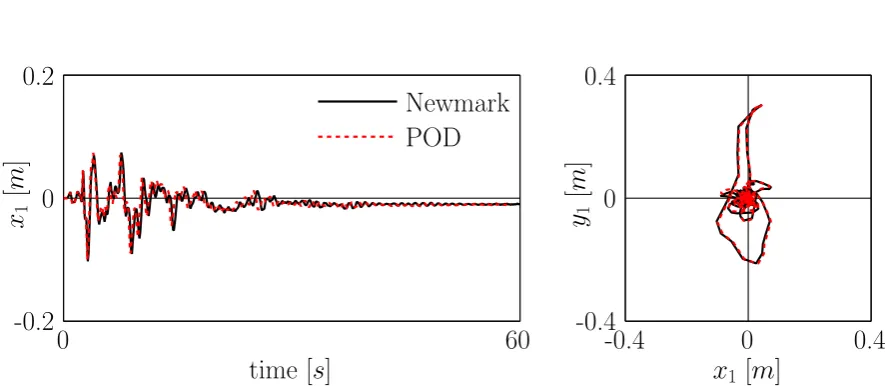
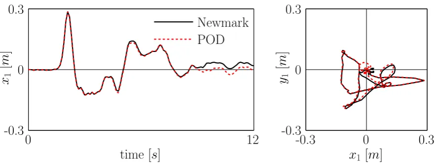
Accurate approximations are achieved by means of the proposed MOR strategy. The re-sponse to the Imperial Valley earthquake (Figure 11), the Landers earthquake (Figure 12) and the North Palm Springs earthquake (Figure 14) were highly accurate, when the proposed MOR strategy was applied. Concerning the response functions of the Loma Prieta (Figure 13) and the North Palm Springs excitation (Figure 15) small variations concerning the full and the reduced solutions can be observed. This is because the responses to those excitations include deforma-tion states that are not captured in the snapshot matrix and, hence, not in the universalPOD modes (POD transformation matrix) and thus cannot assemble the exact response history.

6 Conclusions

0

40

-0.6

0

0.6

time [

s

]

x

[

m

]

-0.6

0

0.6

-0.6

0

0.6

x

[

m

]

y

[

m

]

Newmark

POD

Figure 11: Response functions to the Imperial Valley excitation, full Newmark response and universal reduced POD response; left subplot: displacementxof node1dependent on time; right subplot: movement of the slider, displacementxandyof node1

0

50

-0.5

0

0.5

time [

s

]

x

[

m

]

-0.5

0

0.5

-0.5

0

0.5

x

[

m

]

y

[

m

]

Newmark

POD

0

25

-1

0

1

time [

s

]

x

[

m

]

-1

0

1

-1

0

1

x

[

m

]

y

[

m

]

Newmark

POD

Figure 13: Response functions to the Loma Prieta excitation, full Newmark response and universal reduced POD response; left subplot: displacementxof node1dependent on time; right subplot: movement of the slider, dis-placementxandyof node1

0

60

-0.2

0

0.2

time [

s

]

x

[

m

]

-0.4

0

0.4

-0.4

0

0.4

x

[

m

]

y

[

m

]

Newmark

POD

0

12

-0.3

0

0.3

time [

s

]

x

[

m

]

-0.3

0

0.3

-0.3

0

0.3

x

[

m

]

y

[

m

]

Newmark

POD

Figure 15: Response functions to the Northridge excitation, full Newmark response and universal reduced POD response; left subplot: displacementxof node1dependent on time; right subplot: movement of the slider, dis-placementxandyof node1

model order reduction strategy that is simple in application, but also very effective even in the presence of nonlinearities for problems in the field of earthquake engineering and structural dynamics. This strategy is extended based on the proper orthogonal decomposition (POD) method to derive a proper transformation matrix in order to transform the nonlinear systems into another low-dimensional subspace, which demands considerably less computational effort for the response calculation. Once the transformation matrix is derived, the approach of the strategy is similar to the method of modal truncation for linear systems.

In addition to the development of the MOR strategy, its application for the response cal-culation of a realistic numerical nonlinear example is demonstrated. The example is the dis-placement response calculation of a building structure serving as a medical complex, which is base-isolated by friction pendulum bearing systems excited by six earthquake excitations. In order to evaluate the accuracy of the introduced approach, the exact structural responses were also calculated by the iterative Newmark method in the full order (physical) coordinates. Nu-merical evaluations show that accurate approximations can be achieved if nonlinear response patterns of the structure are already captured in the POD snapshots to extract the transformation matrix. The advantage of this strategy is that obviously the transformation matrix is derived just once and it can be used for response calculation of the structure under different earthquake excitations.

Another substantial advantage of the introduced MOR concerns the speed of the response calculations. Firstly, compared to the basic central difference algorithm, the new introduced strategy has a much larger critical time step. Secondly, compared to the Newmark method, which allows usually larger time steps, no iteration procedure is required.

7 Acknowledgements

REFERENCES

[1] K.J. Bathe,Finite Element Procedures. Prentice Hall, 1995.

[2] Z.Q. Qu, Model order reduction techniques with application in finite element analysis. Springer London Limited, 2004.

[3] G. Rega, H Troger, Dimension Reduction of Dynamical Systems: Methods, Models, Ap-plications.Nonlinear Dynamics,41, 1–15, 2005.

[4] P. Koutsovasilis, M. Beitelschmidt, Comparison of model reduction techniques for large mechanical sytems,Multibody System Dynamics,20, 111–128, 2008.

[5] H.A. Schilders, H.A. Vorst, J. Rommes,Model Order Reducion, Theory, Research Aspects and Application. Springer, 2008.

[6] D. Kosambi, Statistics in function space, Journal of the Indian Mathematical Society, 1943.

[7] K. Karhunen, Uber lineare Methoden in der Wahrscheinlichkeitsrechnung, PhD thesis,¨ University of Helsinki, 1947.

[8] M. Loeve, Fonctions al Eatoire de second ordre,Revue Scientifique,48, 195–206, 1946.

[9] J.P. Cusumano, M.T. Sharkady, B.W. Kimble, Spatial coherence measurements of a chaotic flexible-beam impact oscillator, American Society of Mechanical Engineers, Aerospace Division (Publication) AD,33, 13–22, 1993.

[10] B.F. Feeny, R. Kappagantu, On the physical interpretation of proper orthogonal modes in vibrations,Journal of Sound and Vibration,211, 607–616, 1998.

[11] R. Kappagantu, B.F. Feeny, An “optimal” modal reduction of a system with frictional excitation,Journal of Sound and Vibration,224, 863–877, 1999.

[12] R. Kappagantu, B.F. Feeny, Part 1: Dynamical Characterization of a frictionally excited beam,Nonlinear Dynamics,22, 317–333, 2000.

[13] R. Kappagantu, B.F. Feeny, Part 2: Proper Orthogonal Modal Modeling of a Frictionally Excited Beam,Nonlinear Dynamics,23, 1–11, 2000.

[14] Y.C. Liang, H.P. Lee, S.P. Lim, W.Z. Lin, K.H. Lee, C.G. Wu, Proper Orthogonal De-composition and its Applications - Part 1: Theory,Journal of Sound and Vibration, 252, 527–544, 2002.

[15] G. Kerschen, J.C. Golivani, Physical interpretation of the proper orthogonal modes using the singular value decomposition,Journal of Sound and Vibration,249, 849–865, 2002.

[16] G. Kerschen, J.C. Golivani, A model updating strategy of non-linear vibrating structures, International Journal of Numerical Methods in Engineering,60, 2147–2164, 2003.

[18] F. Bamer, C. Bucher, Application of the proper orthogonal decomposition for linear and nonlinear structures under transient excitation,Acta Mechanica,223, 2549–2563, 2012.

[19] P. Koutsovasilis, M. Beitelschmidt, Comparison of model reduction techniques for large mechanical sytems,Multibody System Dynamics,20, 111–128, 2008.

[20] A.K. Chopra,Dynamics of Structures, Theory and Applications to Earthquake Engineer-ing. Prentice Hall, 2001.

[21] A. Chatterjee, An introduction to the proper orthogonal decomposition,Current Science,

78, 808–817, 2000.

[22] S. Volkwein, Model reduction using proper orthogonal decomposition. Karl-Franzens-Universit¨at Graz, Institut f¨ur Mathematik und Wissenschaftliches Rechnen, 2008.

[23] S. Volkwein, Proper Orthogonal Decomposition and Singular Value Decomposition. Karl-Franzens-Universit¨at Graz, Institut f¨ur Mathematik und Wissenschaftliches Rechnen, 2008.

[24] P. Holmes, J.L. Lumley, G. Berkooz,Turbulence, Coherent Structures, Dynamical Systems and Symmetry. Cambridge University Press, 1996.

[25] S. Han, B. Feeny, Application of proper orthogonal decomposition to structural vibration analysis,Mechanical Systems and Signal Processing,17, 989-1001, 2003.

[26] G. Kerschen, J.C. Golinval, A.F. Vakakis, L.A. Bergman, The Method of Proper Orthog-onal Decomposition for Dynamical Characterization and Order Reduction of Mechanical Systems: An Overview,Nonlinear Dynamics,41, 147–169, 2005.

[27] Z. Qu, Y. Shi, H. Hua, A reduced-order modeling technique for tall buildings with active tunded mass damper, Earthquake Engineering and Structural Dynamics, 30, 349–362, 2001.

[28] A.G. Schemann, H.A. Smith. Vibration control of cable-stayed bridges - part 1: modelling issues,Earthquake Engineering and Structural Dynamics,27, 811–824, 1998.

[29] E. Gutierrez, J.M. Zaldivar, The application of Karhunen-Loeve, or principal component analysis method, to study the non-linear seismic response of structures,Earthquake Engi-neering and Structural Dynamics,29, 1261–1286, 2000.

[30] E. Gutierrez, J.J.L. Cela, Improving explicit time integration by modal truncation tech-niques,Earthquake Engineering And Structural Dynamics,27, 1541–1557, 1998.

[31] Pacific Earthquake Engineering Research Center (PEER), Homepage: http://nisee.berkeley.edu, 2015.

[32] C. Bucher, Stabilization of explicit time integration by modal reduction,Trends in compu-tational structural mechanics, 2001.

[34] J. Llera, J. Almazan, An experimental study of nominally symmetric and asymmetric structures isolated with the FPS,Earthquake Engineering and Structural Dynamics, 32, 891–918, 2003.

[35] D. Ordonez, D. Foti, L. Bozzo, Comparative study of the inelastic response of base isolated buildings,Earthquake Engineering and Structural Dynamics,32, 151–164, 2003.

[36] K. Ryan, A.K. Chopra, Estimating the seismic displacement of friction pendulum isolators based on non-linear response history analysis, Earthquake Engineering and Structural Dynamics,33, 359–373, 2004.

[37] T. Ray, A. Sarlis, A. Reinhorn, M. Constantinou, Hysteretic models for sliding bear-ings with varying frictional force,Earthquake Engineering and Structural Dynamics,42, 2341–2360, 2013.

[38] C. Bucher, Probability-based optimal design of friction-based seismic isolation devices, Structural Safety,31, 500–507, 2009.

[39] C. Bucher, Open source structural dynamics and FE software (slangTNG), Homepage: http://info.tuwien.ac.at/bucher/Private/Welcome.html, 2015.