Planetary micro-rover operations on Mars using a Bayesian framework for inference and control

Planetary Micro-Rover Operations on Mars Using a

Bayesian Framework for Inference and Control

Mark A. Post

_{, Junquan Li}

_{, Brendan M. Quine}

a

Space Mechatronic Systems Technology Laboratory, Department of Design, Manufacture and Engineering Management, University of Strathclyde, 75 Montrose St. Glasgow,

United Kingdom. G1 1XJ +44-(0)141-574-5274

b

Department of Earth and Space Science and Engineering, York University, 4700 Keele Street, Toronto, ON, Canada. M3J 1P3 +1(416)736-2100 x22095

Abstract

With the recent progress toward the application of commercially-available

hardware to small-scale space missions, it is now becoming feasible for groups

of small, efficient robots based on low-power embedded hardware to perform

simple tasks on other planets in the place of large-scale, heavy and expensive

robots. In this paper, we describe design and programming of the Beaver

micro-rover developed for Northern Light, a Canadian initiative to send a

small lander and rover to Mars to study the Martian surface and

subsur-face. For a small, hardware-limited rover to handle an uncertain and mostly

unknown environment without constant management by human operators,

we use a Bayesian network of discrete random variables as an abstraction of

expert knowledge about the rover and its environment, and inference

opera-tions for control. A framework for efficient construction and inference into a

Bayesian network using only the C language and fixed-point mathematics on

embedded hardware has been developed for the Beaver to make intelligent

decisions with minimal sensor data. We study the performance of the Beaver

as it probabilistically maps a simple outdoor environment with sensor models

that include uncertainty. Results indicate that the Beaver and other small

and simple robotic platforms can make use of a Bayesian network to make

intelligent decisions in uncertain planetary environments.

∗_{Corresponding author}

Email addresses: mark.post@strath.ac.uk(Mark A. Post),junquanl@yorku.ca

(Junquan Li), bquine@yorku.ca(Brendan M. Quine)

*Manuscript

Keywords:

Planetary Micro-Rover Operations on Mars Using a

Bayesian Framework for Inference and Control

Mark A. Postc,∗_{, Junquan Li}d_{, Brendan M. Quine}d

c

Space Mechatronic Systems Technology Laboratory, Department of Design, Manufacture and Engineering Management, University of Strathclyde, 75 Montrose St. Glasgow,

United Kingdom. G1 1XJ +44-(0)141-574-5274

d

Department of Earth and Space Science and Engineering, York University, 4700 Keele Street, Toronto, ON, Canada. M3J 1P3 +1(416)736-2100 x22095

1. Introduction

Intelligent autonomous operation is easily the most difficult problem in mobile robotics. While known and finite sets of conditions can be planned for and responses pre-programmed using a variety of methods, giving a robot the ability to appropriately handle unexpected and uncertain circumstances remains an open and very challenging problem. Planetary rovers would easily benefit the most from full autonomy, given that they must operate in uncer-tain conditions while isolated from any direct human assistance. Ceruncer-tainly real-time control of a rover on another planet is infeasible, as the delay in communicating a signal to Mars at the speed of light ranges from 3 to 21 minutes, not even considering temporary communications blackouts and time for retransmitting due to packet errors. However, due to the complexities in-volved, autonomy on space hardware has been very slow in adoption because of the inherent risks of autonomy failures with the extremely high costs of putting space hardware on other planets. Rovers work in a partially un-known environment, with narrow energy/time/movement constraints and, typically, limited computational resources that limit the complexity of on-line planning and scheduling. This is particularly true of micro-rovers and other small, inexpensive robots that are desirable to reduce potential losses if

∗_{Corresponding author}

problems occur with individual units, but require low-power embedded sys-tems for control that over long periods will need to adapt to unknowns in less reliable hardware like mechanical wear, system failures, and changes in envi-ronmental conditions. Considerable research work has been done on efficient planning algorithms [1] and algorithms to autonomously modify planning to handle unexpected problems or opportunities [2]. In particular, probabilistic methods have been used to great effect [3]. Adaptive learning and statistical control is already available for planetary rover prototypes, and can be signif-icantly improved to decrease the amount of planning needed from humans [4], but is still often underutilized.

1.1. Bayesian Reasoning

Bayesian Networks (BN) are well-suited for handling uncertainty in cause-effect relations, and handle dependence/independence relationships well pro-vided that the network is constructed using valid relational assumptions.

Gallant et al. [5] show how a simple Bayesian network can operate to

determine the most likely type of rock being sensed given a basic set of sensor data and some probabilistic knowledge of geology. To make it pos-sible for the small, efficient planetary rovers of the future be decisionally self-sufficient, focus is needed on the design and implementation of efficient but robust embedded decision-making systems for tasks such as navigation and identification. Some drawbacks of this method are that the variables, events, and values available must be well-defined from the beginning, and the causal relationships and conditional probabilities must be available ini-tially [6]. This makes construction of the Bayesian network a considerable challenge. Bayesian networks have been used extensively for image recogni-tion, diagnostic systems, and machine behaviours. However, the potential of these concepts for distributed machine learning and problem-solving is considerable, and warrants further real-world research. In the reference [7], a self-organized control method for a planetary rover has been studied, but only extends to the navigation problem.

the measurement made is estimated, mapped in the same way, and used to drive the search pattern. A set of behaviours is then applied to the likelihood map to implement obstacle avoidance. To evaluate performance in a real-world scenario, this system is implemented on a small micro-rover prototype and tested in an outdoor area with obstacles present. The use of a common Bayesian framework simplifies operational design and calculation methods throughout the whole system. Following this Section 1, Section 2 provides background information on Bayesian networks and inference methods in the context of discrete reasoning, Section 3 explains our implementation of a Bayesian network and compares our methodology to the original concept of Bayesian Robot Programming as described by Lebeltel et al., Section 4 de-tails the design and methodology of a simple obstacle mapping system using the Bayesian framework, and Section 5 shows the results of actual testing using this system. Section 6 then concludes the paper.

1.2. The Beaver µrover

The original application for development of our probabilistic system is the Northern Light mission, a Canadian initiative to send a lander such as the one shown in Figure 1 to the surface of Mars for a short-range mission to observe the surface and position a ground-penetrating radar at a distance from the lander module for subsurface imaging [8]. For this purpose, it is planned to include a micro-robot, known as the Beaver rover, which will leave the lander and perform geological surveying and imaging of the Mar-tian surface. The primary science payloads for this mission are an Argus infrared spectrometer for spectral analysis of surface rocks, the same type as is currently used on the CANX-2 Nanosatellite for atmospheric imaging, and a ground-penetrating radar system, which is currently under parallel de-velopment. For this mission, the Beaver will have to traverse a distance of under a kilometre while avoiding obstacles and taking sensor measurements. Naturally, extended and reliable operation on the surface of Mars would be preferred.

The Beaver micro-rover (µrover) prototype currently in use was developed

for this mission as a stand-alone, self-powered, autonomous ground roving vehicle of 6kg mass designed to gather data and perform simple tasks in dis-tant or hostile environments such as Mars, the Moon, or here on Earth [9].

The µrover is powered from solar panels and can recharge outdoors while

Figure 1: Northern Light Lander Module (Air Whistle Media/Thoth Technology Inc.)

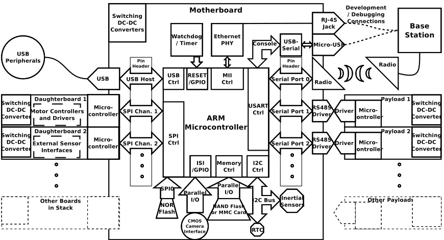
makes it very flexible and useable for both planetary and terrestrial research purposes [10]. It has a power-efficient ARM-based onboard computer, a color CMOS camera, magnetometer, accelerometer, six navigational infrared sen-sors, and communicates via long-range 900MHz mesh networking. A variety of communications interfaces including RS-485 serial, SPI, I2C, Ethernet and USB are used for payload interfacing [11]. A diagram of the onboard sys-tems available is shown in Figure 2, and the electronics are implemented in a PC/104+ form factor stack with external payload connectors. Program-ming is done in the C language using fixed-point numerical processing for efficiency. The autonomy algorithms are probabilistic in nature, using adap-tive Kalman filtering [12] and Bayesian networks to handle uncertainty in the environment with minimal computation requirements. The Beaver uses probabilistic methods for mission planning, operations, and problem-solving, where each state variable in the system is considered to be a random variable. Localization and motion tracking is performed on two scales. For short distances, high-precision tracking is performed using an HMC5883L mag-netometer as a compass to obtain heading information, and a downward-pointing optical sensor to monitor horizontal motion [13]. The optical sensor is calibrated using reference distances obtained from encoders on the drive

periodi-Figure 2: Beaver Micro-rover Modular Electronic Systems

cally updated with the position obtained from a Trimble Lassen IQ GPS unit

to identify and correct accumulated positional error. A resolution of 0.5m

is used for the occupancy grid as this follows the current level of accuracy of the GPS position estimation system. Rollover risk and terrain variations are handled with a nonlinear controller that adjusts the suspension angle by using differential torques from the four drive motors to raise, lower, and tilt the suspension as needed. A monocular vision system has also been devel-oped to augment the mapping of terrain by building feature maps in three dimensions by triangulation of features detected by the ORB algorithm us-ing a dedicated DSP board for vision. [15] [16]. As localization methods are improved, eventually the GPS will not be needed for navigation of the

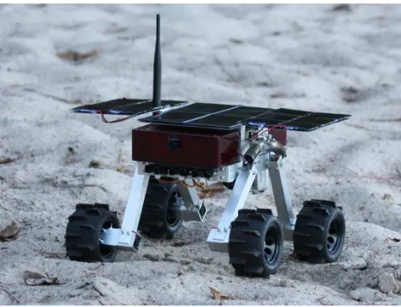
micro-rover. A picture of the Beaverµrover under testing in a sandy outdoor

environment is shown in Figure 3.

2. Methods

Figure 3: Beaverµrover Prototype Testing in Sand

contrast to “definite” variables that have a certain known or unknown value. In a stochastic system, states are determined by the probability distributions in random variables, where the values that a random variable takes on have precise probabilities associated with them, and the sum (or integral) of all probabilities in a random variable is defined to be 1 to reflect that there must be some value associated with the random variable that is present. Proba-bility theory provides a framework for logically handling random variables and the relationships between them so that useful results can be determined. Logically connecting many random variables together based on probabilistic dependencies requires the concept of “evidence”, on which a change in a given set of probabilities can be based. The interpretation of Bayesian probabil-ity makes use of propositional logic to enable “hypotheses” to be tested and updated based on probabilistic data. This process of “Bayesian inference” is central to our treatment of probabilistic systems. The term “Bayesian” refers to the 18th century statistical theologian and Presbyterian minister Thomas Bayes, who formulated the basic theorem of statistical inference based on conditional probability.

Bayesian networks are similar in concept to fuzzy systems, but have one

whereas probabilities are precisely defined but may change when an event

oc-curs. Rather than characterize a variable as having partial memberships,

probabilistic or “random” variables can only have one value, but with a cer-tain probability that varies depending on other factors. These other factors can be probabilities themselves, leading to the concept of a Bayesian net-work of conditional probabilities. Probability in this case implies directed

causality a_→b _→c, and Bayesian networks allow associations to be defined

to determine the likelihood of both a and b if c is known. Using associated

probabilities allows a machine learning system to calculate not only what specific actions should have a certain effect, but what actions are unlikely to have that effect, and also what actions may have already had that effect or not. This ability to characterize multiple causes and “explain away” unlikely causes makes a Bayesian network a very powerful predictive tool.

2.1. Naive Bayesian Modelling

The most useful contribution of Bayesian networks to real probability calculations is reducing the storage and computation required. A joint

prob-ability distribution P(X1, . . . , XL) for random variables with N values

re-quires NL

−1 separate probability values to store allNL _{combinations of the}

values in all variables with related probability data for each combination. By exploiting independence between random variables, we can parameterize the

distribution into a set of specific outcomes. For example, if we let Xm be

the result of a coin toss out ofM coin tosses with two possible values forxm

being X =xheads and X =xtails, we can define the parameterized

probabil-ity pm as the probability that the m’th coin toss results in heads. Using the

probabilities P(X = xheads) = 0.5 = pm and P(X = xtails) = 1−0.5 = 0.5,

we can now represent the distribution using only the M values of pm rather

than all 2M _{possible combinations of random variable values. The critical}

assumption is that each random variable is at least marginally independent

of the other variables, which allows us to write the distribution over M coin

tosses as

P(X =x1, X =x2, . . . , X =xM) (1)

= P(X =x1)P(X =x2). . .P(X =xM) = M Y

m=1

pm.

storage and calculation more tractable. However, obtaining useful probabil-ity estimations for use in a joint distribution is not trivial. Most commonly,

probability estimates for values of random variables such as X and Y are

obtained through averaging of repeated trial measurements of the stochas-tic processes they represent. The probability values in a joint distribution

P(X, Y) can be completely different from those in the separate marginal

dis-tributions P(X) and P(Y). Given a large enough database of experience,

it may be possible to estimate the joint distribution completely, but there is little information that can be re-used and every joint distribution would require a separate dataset. It is much more practical to use the chain rule for conditional random variables to factor the distribution into a conditional probability

P(X, Y) = P(X)P(Y_|X). (2)

Of course, this example only considers a single relationship, and proba-bilistic models of much more complicated systems are needed, with multiple probability dependencies. For example, a vision system operating in concert with the obstacle sensor may be able to detect and triangulate features on nearby objects, and we can use it to increase the accuracy of our

estima-tion of object presence. Let W be the random variable of features being

detected within the range of the obstacle sensor, and let P(W = wf) be

the parameterized probability that enough features are detected to consti-tute an obstacle. For the moment, we need not consider the complexities of determining whether the features in question constitute an obstacle, as this complexity can be effectively “hidden” by the use of the distribution over

W, as we will clarify later. It is natural to think of the information from

these two sensors as being related (and hence the variablesW and X), since

they are effectively observing the same set of obstacles. We can write the conditional joint distribution over these two variables similarly to Equation 2 as

P(W, X, Y) = P(W, X_|Y)P(Y) (3)

= P(W_|Y)P(X_|Y)P(Y).

In this way, we can generalize the factorization of a joint distribution of

M variablesX1. . . XM that are marginally independent but dependent on a

P(X1, . . . , XM, Z) = P(Z) M Y

m=1

P(Xm|Z). (4)

This principle of factorizing parameterized joint distributions is extremely useful. Besides being able to “split up” a joint distribution into more

easily-obtainable conditional factors, if we assume N values for each random

vari-able we can again reduce the number of actual probabilities required across

M random variables from the order ofNM _{+ 1 to the order ofN}

×M+ 1 by

means of parameterization, as well as correspondingly reducing the amount

of calculation required to a set of multiplications. If P(W_|Y) and P(X_|Y) are

considered to be “likelihoods” and P(Y) is a “prior”, then only “evidence”

is missing from this expression, indicating that for our example we are only describing a probability of general object detection and the actual reading

of the sensor is missing. If we divide both sides of Equation 4 by P(X) and

apply the chain rule so that P(W, X, Y)/P(X) = P(W, Y_|X), we return to a

conditional expression that has a change of dependency on the left hand side

P(W, Y_|X) = P(W|Y)P(X|Y)P(Y)

P(X) . (5)

The sensory model we describe here is consequently known as a naive Bayes model, which is often used for classification of observed features in sensory systems. For these systems, it is assumed that the conditional

vari-able Y contains a set of “classes” that are responsible for the “features”

represented by variables X1. . . XM. If we want to compute a measure of

confidence in whether a class y1 or y2 better fit the observed features, we

can compare two distributions directly by taking the ratio of their posterior probability distributions

P(X1 =x1, . . . , XM =xm, Y =y1)

P(X1 =x1, . . . , XM =xm, Y =y2)

(6)

= P(Y =y1)

P(Y =y2)

M Y

m=1

P(Xm|Y =y1)

(Xm|Y =y2)

.

As we now have methods for building probabilistic relationships and mak-ing probabilistic inferences, we can make use of this framework to allow a

situations. The basis for our approach is inference using a Bayesian network as an abstraction of expert knowledge regarding the rover itself and assump-tions about its environment, such as obstacles and hazards. We approach the problem of probabilistic robotics using the Bayesian Robot Programming (BRP) methodology developed by Lebeltel, Bessiere et al [17] [18] [19], which provides a quite comprehensive framework for robotic decision-making using inference and learning from experience. Despite having considerable promise and providing a novel solution for reasoning under uncertainty, BRP has not been developed significantly since the initial publications during 2000-2004. We add to this method by formally using Bayesian networks as a knowledge representation structure for programming, and by constructing these

net-works dynamically with implicit information obtained from the µrover bus

and from a store of mission information. There are several advantages to this approach, which include clarity of representation, a practical structure for constructing joint distributions dynamically, and reliance on a proven probabilistic methodology. Also, the use of recursive inference in a Bayesian network avoids the need to manually partition and decompose large joint distributions, which greatly simplifies the programming process.

2.2. Bayesian Networks

For us to be able to properly organize and represent a large set of joint distributions using factorization in this way, we need a method of clearly associating random variables that are dependent on each other. Using the naive Bayes model for random variable dependence, a directed graph can be constructed, with nodes that represent random variables connected by edges that show the direction of dependence of one random variable on another. A graph or “network” of probability distributions over random variables, with one independent random variable representing a node and directed edges showing its dependencies, is called a Bayesian Network (BN), and forms the representation of our probabilistic relationships.

A Bayesian Network (BN) can be visualized as a directed acyclic graph (DAG) which defines a factorization (links) of a joint probability distribu-tion over several variables (nodes). The probability distribudistribu-tion over discrete variables is the product of conditional probabilities (“rules”). For a causal

statement X _→Y often it is needed to find P(X_|Y =y) using the

P(X_|Y =y) = P(Y =y|X)P(X)

P(Y =y) . (7)

and a Bayesian network, when viewed from the point of view of a single joint probability distribution, can be represented by:

P(X1· · ·Xn) =

n Y

i=1

P(Xi|Pa(Xi)) (8)

where the parents or depended-on variables) of eachi’th nodeXi are denoted

by Pa(Xi). To construct a BN, you identify the variables and their causal

relationships and construct a DAG that specifies the dependence and inde-pendence assumptions about the joint probability distributions. Bayesian networks can be constructed using semi-automated means if there is infor-mation regarding the probability and independence of network variables. We construct the Bayesian network with information about the components of the rover itself and the mission plan, where causality is implicit as the struc-ture is broken down into components and sub-components. Applying the chain rule for conditional probabilities [20], to all nodes in a Bayesian net-work, the probability distribution over a given network or subnetwork of

nodes ℘ =_{X1. . . XM} can be said to factorize over ℘ according to the

de-pendencies in the network if the distribution can be expressed as a product

P(_{X1. . . XM}) = M Y

m=1

P(Xm|P a(Xm)). (9)

The chain rule is particularly useful for calculating the Conditional Prob-ability Distribution (CPD) of a given node in the network. Due to the

depen-dency structure of the network, the conditional probability of a given nodeX

depends on all its ancestors, so that P(X_|Pa(X)) must be calculated

recur-sively. A query for the posterior probability distribution of X involves first

querying all of its parent nodes Y _∈ Pa(X) to determine their probability

distributions, then multiplying them by the probability distributions of each

parent node Y such that by a simplification of the chain rule

P(X =x) = X

Y∈Pa(X)

P(X =x_|Y =y)P(Y =y). (10)

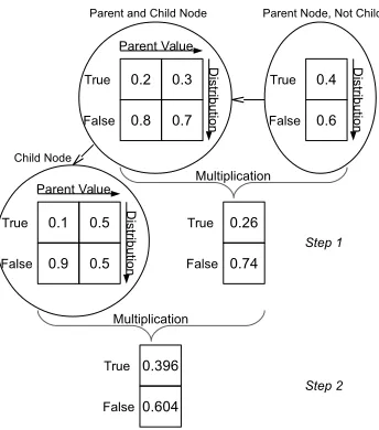
Figure 4: Matrix Calculation for Querying a Random Variable with One Parent

matrix multiplication. This process is graphically illustrated in Figure 4. The

CPD P(X) represents a local probabilistic model within the network, which

for each node represents a local summary of probability for its own random variables. For a continuous distribution, it can be a function evaluation.

Representing probability distributions by tables, the distribution P(X_|Y)

will be an L+ 1-dimensional matrix forLparents, with the major dimension

of sizeN forN random variable values in V(X). Each parentY is assumed to

have a distribution of sizeM (although each could be different with no change

in the concept), so that the distribution P(Y) is a N _×1 matrix. For nodes

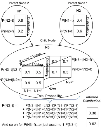
with two or more parents. the process is more complex, as each possible value of the inferred distribution must be calculated as a sum of the probabilities that lead to that value, as shown in Figure 5. To calculate the conditional

distribution for X, the size M _×N plane of the matrix representing the

values from the parent versus the values from the child node, which is the

distribution P(X_|Y) is multiplied with the N _×1 distribution P(Y). This

results in anN_×1 matrix that is effectively a temporary posterior distribution

estimate for P(X) which avoids frequent recalculation for determining the

conditional distributions of children Ch(X) while traversing the network.

Figure 5: Matrix Calculation for Querying a Random Variable with more than One Parent

into a Bayesian network is widely understood to be an NP-hard problem [21] [22], it is still much more efficient than the raw computation of a joint distribution, and provides an intuitive, graphical method of representing de-pendencies and independences. It is easy to see how any system that can be described as a set of independent but conditional random variables can be abstracted into a Bayesian network, and that a wealth of information regarding the probability distributions therein can be extracted relatively efficiently. This forms our basic methodology for probabilistic modelling.

P(X1∩X2∩. . .∩XN) (11) = P(X1)P(X2|X1). . .P(XN|X1∩. . .∩Xn₋1).

This allows any number of events to be related in terms of other events, and is a very important result for inference systems. The order or numbering

of the events is not important because the conjunction operator_∩is

for a conditional probability that provides a degree of confidence in a certain event with respect to other known events.

P(Y_|X) = P(X|Y)P(Y)

P(X) (12)

= (likelihood)·(prior) (evidence) .

2.3. Probability Queries

Once a probability distribution is defined, it is necessary to have a con-sistent method of extracting information from it. In most cases, rather than knowing the entire probability distribution, we only are interested in a specific probability of a single value or set of values, usually the highest probability. This is referred to as a Maximum A Posteriori (MAP) query, or alternately, “Most Probable Explanation” (MPE). This refers to the most likely values of all variables that are not used as evidence (because evidence is already

known and has certain probability), and is described using arg maxxP(x)

(the value of x for which P(x) is maximal) as

MAP(X_|Y =y) = arg max

x P(x∩y). (13)

A very important point to note is that while the MAP query for a single

variable MAP(X_|Y =y) is equivalent to just finding the highest probability

of the single-variable distribution P(X), it is not the same as finding all the

maximum values in a joint conditional distribution P(X _∩Z), because the

underlying probabilities in this joint distribution depend on both values ofX

and Z. Rather, a MAP query over a joint distribution finds the most likely

complete set of values (x, z) as each combination of values has a different

probability. This leads to an important generalization of the MAP query,

in which we use a smaller subset of X to find a less likely set of events by

independently searching a joint, conditional distribution of the subset. This is called a marginal MAP query, and is used frequently in Bayesian inference engines.

MAP(X_|Y =y) = arg max

x X

Z

2.4. Logical Propositions

Inference in Bayesian programming generally relies on the concept of log-ical propositions. A loglog-ical proposition is essentially a formalization of the state of a probabilistic system, which by our probabilistic framework is

repre-sented by a value assignment for a discrete random variableX =xor several

discrete random variables. Conjunctions (X = x_∩Y =y) and disjunctions

(X =x_∪Y =y) are then also, by extension, propositions. To distinguish the

use of random variable sets from the use of propositions (although logically, sets and propositions are isomorphic to each other) we will use the

proposi-tional logic operators _∧ for conjunction and_∨ for disjunction, as well as the

shorthand notation for random variables. Hence, propositions will take the

form (x), (x_∧y), and (x_∨y). We add to this the concept of the negation of a

proposition _¬x, which represents the complement of the valuex. For a

prob-ability assignment P(X=x), this represents the complementary probability

1₋P(X =x), or informally, the probability of a given event not happening.

As with Bayesian networks, the process of inference is used to extract in-formation from propositions, based on conditional probability distributions over a set of random variable dependencies. It is assumed that most propo-sitions are conditional on the same basic set of prior knowledge (or in graph parlance, the random variables most queried are child nodes of the same set of parent nodes). The conjunction of the set of random variables that are considered “prior knowledge” for a given proposition are often shortened to

the propositionπfor brevity, and can be thought of in a Bayesian network as

parents of the node being examined. Based on the rules used for probabilistic inference, only two basic rules are needed for reasoning [23]: the Conjunc-tion Rule and the NormalizaConjunc-tion Rule. We assume that the random variables

used such as X are discrete with a countable number of values, and that a

logical proposition of random variables [X = xi] is mutually exclusive such

that _∀i ₆= j,_¬(X = xi ∧X = xj) and exhaustive such that ∃X,(X = xi).

The probability distribution over a conjunction of two such variables using

shorthand notation is then defined as the set P(X, Y)_≡P(X =xi∧Y =yi).

Using this concept of propositions, the Conjunction and Normalization Rules are stated as [17]

∀xi ∈X,∀yj ∈Y : P(xi∧yj|π) = P(xi, yj|π) (15)

= P(xi|π)P(yj|xi, π) = P(yj|π)P(xi|yj, π)

∀xi ∈X,∀yj ∈Y : P(xi ∨yj|π) (16)

= P(xi|π) + P(yj|π)−P(yj|π)P(xi, yj|π)

while the Normalization Rule becomes

∀yj ∈Y :

X

∀xi∈X

P(xi|π) = 1. (17)

The marginalization rule may then be derived for propositions as

∀yj ∈Y :

X

∀xi∈X

P(xi, yj|π) = P(yj|π). (18)

For clarity, when applying these rules to distributions over random vari-ables, we do not necessarily have to state the individual propositions (or values). As with common random variable notation, the conjunction rule can be stated without loss of generality as

P(X, Y_|π) = P(X_|π)P(Y_|X, π), (19)

the normalization rule as

X

X

P(X_|π) = 1, (20)

and the marginalization rule as

X

X

P(X, Y_|π) = P(Y_|π). (21)

It is assumed that all propositions represented by the random variable follow these rules.

3. Theory and Implementation

There are many existing software packages for building and using Bayesian

networks, but forµrovers we require a a software framework that is portable,

highly resource-efficient, and usable on embedded systems, as well as

be-ing accessible and open for development. The µrover does not run Java or

support Python), and the need for simple integration at a low level with other robotic components makes the use of a MATLAB embedded target binary impractical. Due to the constraints involved in running Bayesian in-ference processes on low-power ARM hardware and the need to adopt other architectures in the future, the C language was chosen as the lowest common denominator for compatibility between systems despite the extra complexity required for implementation in such a low level language. C++ bindings are also planned for development in order to make interfacing with other programs easier. The original framework for Bayesian Robot Programming, known as Open Probabilistic Language (OPL), was originally made available freely [18] but was later renamed and redistributed as a proprietary package called ProBT [19]. Several other currently-maintained and open-source

pack-ages were considered for use on the µrover, such as Bayes++, Mocapy++,

and LibDAI, which is a recent but promising system for inference [24]. How-ever, there is no known general framework that is implemented in bare C for

efficiency and portability as is preferred for µrover software, and is focused

specifically on robotic use in embedded systems, particularly with consider-ation to fixed-point math. It was therefore determined that a new Bayesian

inference engine for the µrover had to be created.

3.1. Bayesian Robot Programming

A Bayesian program has been defined by Lebeltel et al. as a group of probability distributions selected so as to allow control of a robot to per-form tasks related to those distributions [17]. A “Program” is constructed from a “Question” that is posed to a “Description”. The “Description” in

turn includes both “Data” represented by δ, and “Preliminary Knowledge

represented by π. This “Preliminary Knowledge π consists of the pertinent

random variables, their joint decomposition by the chain rule, and “Forms” representing the actual form of the distribution over a specific random vari-able, which can either be parametric forms such as Gaussian distributions with a given mean and standard deviation, or programs for obtaining the distribution based on inputs [18]. Rather than unstructured groups of

vari-ables, we apply these concepts to a Bayesian network of M random variables

℘ =X1, X2, . . . , XN ∈π, δ, from which an arbitrary joint distribution can be computed using conjunctions. It is assumed that any conditional

indepen-dence of random variables in π and δ (which must exist, though it was not

for joint distributions. The general process we use for Bayesian programming, including changes from the original BRP, is as follows:

1. Define the set of relevant variables. We use the edges between nodes to represent dependencies. For example, for a collision-avoidance program, the relevant variables include those from the nodes associated with the obstacle sensors and vision system, and are generally easy to identify due to the structure of the network. Usually, a single child node is queried to include information from all related nodes.

2. Decompose the joint distribution. Rather than partitioning

vari-ables P(X1, . . . , XM|δ, π) into subsets [19], we make use of the

prop-erties of the Bayesian network for implicitly including information in parent nodes when queried. A question such as a MAP query of any given node involves knowing the distributions for the parents of that node, and so on recursively until a node with no parents is reached, by

P(X)QM

m=1P(Xm|δ, π).

3. Define the forms. For actual computations, the joint and dependent distributions must be numerically defined. The most common function to be used, and the function used for distributions in this work, is the

Gaussian distribution with parameters mean ¯xand standard deviation

σ that define the shape of the distribution, commonly formulated as

P(X =x) = _σ√1

2πe

−(x−x¯)2 2σ2 .

4. Formulate the question. While queries into a BRP system tradition-ally involve partitioning random variables into three sets: “searched”

(Se), “known” (Kn), and “unknown” (Un) variables. The use of a

Bayesian network formalizes the relationships of these sets, so that “searched” nodes can be queried, and implicitly will include all rele-vant known and unknown information in the network. It is important to note that a “question” is functionally just another conditional distri-bution, and therefore operates in the same way as an additional node in the Bayesian network.

5. Perform Bayesian inference. To perform inference into the joint distribution, the “Question” that has been formulated as a conjunction

a Bayesian inference. The “Answer” is obtained as a probability dis-tribution, or in the case of a MAP query, a value from the “searched” variable. For our Bayesian network implementation, nodes associated with actions to be taken typically have conditional distributions that act as “questions” regarding their operational state.

3.2. Bayesian Inference

The last step in Bayesian programming is the actual inference operation used to determine the probability distribution for the variable or set of

vari-ables in question. Obtaining the joint distribution P(Se_|Kn, π) is the goal,

and requires information from all related random variables in _{Kn, Un, π_},

which in the Bayesian network are visualized as parents ofSe. This

distribu-tion can always be obtained using the following inference method [25]. The

marginalization rule from Equation 21 first allows the inclusion of Un, as

P(Se_|Kn, δ, π) =X U n

P(Se, Un_|Kn, δ, π). (22)

By the conjunction rule from Equation 19, this can be stated as

P(Se_|Kn, δ, π) = P

U nP(Se, Un, Kn|δ, π)

P(Kn_|δ, π) . (23)

Applying the marginalization rule again to sum the denominator over

both Se and Un, we have

P(Se_|Kn, δ, π) = P

U nP(Se, Un, Kn|δ, π) P

{Se,U n}P(Se, Un, Kn|δ, π)

. (24)

The denominator of Equation 24 acts as a normalization term, and for

simplicity will be replaced with the constant Σ =P

{Se,U n_}P(Se, Un, Kn|δ, π), giving

P(Se_|Kn, δ, π) = 1 Σ

X

U n

P(Se, Un, Kn_|δ, π). (25)

To complete the inference calculation, we only need to reduce the

distri-bution P

this, we must assume that these factors are at least marginally independent. While BRP originally reduced these factors into marginally independent sub-sets, we can assume that independence is denoted by the structure of the

Bayesian network, so we only need be concerned with the ancestors of Se.

Using only the ancestors of a given node removes the need to scale by Σ. Given that inference into a Bayesian network typically involves querying a

single node, we will assume that Se is the singleton Se = _{X_}. This can

also be accomplished ifSe is larger by makingX a parent of all nodes inSe.

Applying the chain rule again to Bayesian networks, the probability

distri-bution over Sedirectly depends on the distributions of its parents, which for

the moment we will assume are known to be unconditional random variables

for clarity. We can factorize the immediate vicinity of Se=_{X_} as

P(Se_|Kn, δ, π) = X U n

Y

Y∈{X,Pa(X)}

P(X_|Y)P(Y). (26)

This gives us a factorization for a single node. Of course, we cannot

assume that the parents of X have no dependencies, and in general should

be assumed to have some other dependencies Z so that we have P(Y_|Z). In

this case we must consider the parent nodes of the node being queried Pa(X),

the parents of the parent nodes Pa(Pa(X)), and so on recursively until we

have spanned the complete set of ancestors Y with Y _∈ An(X). From a

purely algorithmic perspective, we can walk the Bayesian network backwards

through the directed edges from X, determining the conditional distribution

of each node from its parents as we go, and therefore breaking down the determination of the joint distribution into smaller, separate calculations.

Considering Z to be the parents of each ancestor node Y and following the

method of Equations 9, Equation 10, and Equation 26, a general expression

for the factorization of P(Se_|Kn, δ, π) through the Bayesian network is

P(Se_|Kn, δ, π) = X Y_∈{X,An(X)



 Y

Z_∈Pa(Y)

P(Y_|Z)P(Z)



. (27)

This is a recursive calculation, as we must first obtain the conditional

distributionsP(Z_|Y) for the ancestorsZ furthest from the nodeXbefore the

closer ancestors and parents of X (as in depth-first traversal of the branches

of a dependency tree). To save calculations, the temporary estimate P(Y) =

the children of Y.

To construct an appropriate machine representation of a Bayesian net-work, it is necessary to consider both the numerical properties of a Bayesian node (or random variable), and the underlying requirements of the hardware and software that support the information contained in the network. As Bayesian nodes are essentially random variables associated with other ran-dom variables by way of a joint distribution, an object-oriented approach is taken to describing them using C structures. Unlike most Bayesian network implementations, our implementation is unique in that it uses fixed-point math for storage and calculation and is programmed in C for better porta-bility and calculation efficiency on small-scale embedded systems.

3.3. Programming the Bayesian Network

The fundamental properties of a Bayesian Node are the probability dis-tribution of the random variable, and the way that disdis-tribution is affected by the knowledge of other nodes nearby. For numerical compactness and

code efficiency, the values of a node are represented as M _×N distribution

matrices, where each row represents the probability distribution of the ran-dom variable, and each column represents the effects of linked nodes. Total

probability requires that all values in each row m sum to 1. The joint

dis-tribution P of probability values associated with a given random variable is the content actually stored, as well as a vector of labels for each of the local values in the random variable itself.

At minimum, a random variable withN possible values will have a 1_×N

distribution matrix. A parent node will increase the number of distributions

that must be accounted for in the child node, causing at most M possible

probability distributions for each one of its M possible variable values. If

two or more parent nodes are present, the total number of combinations of affecting values must be considered in the child node. Hence, a parent with 2

values and a parent with 3 values will together contribute 2_×3 = 6 possible

probability distributions, and if the node itself has 4 possible values, a total

of 4_×2_×3 = 24 probability values must be stored in total. In general, if each

parent has a distribution Nl values in size, and there areL parents, then the

number of distributions M possible in the child node are

M =

L Y

l=1

As each child node must have an N _×M matrix, assuming that parent nodes have similar numbers of values, the storage size of the node scales

roughly as NL_{. This can be mitigated by designing a deeper graph with}

more nodes and less parents per node, as the simplifying properties of the Bayesian network will decrease the total storage required. A parent node

with anMl×Nl distribution matrix, regardless of the number of parents and

the size of Ml, will still only contribute Nl values to its child nodes, making

the speed of storage size increase dependent on the size of the probability

distributions in question. A given node X will then have to store a table of

size _|V(X_∪Pa(X))_|.

The actual method of storing the distributions is not trivial. Because the dimensionality of the distribution matrix effectively increases with each par-ent (adding a new set of combinations of variables), fixed-dimension matrices are not practical for nodes where new parents may have to be added dynam-ically. Many languages use nested template classes and other object-oriented methods for implementing N-dimensional storage. However, for speed and compactness of storage, we use a single C array for storage of the distri-bution, and index it with a linear index that is a function of the parent numbers of the node. To create the index, when addressing an array as an

L+ 1-dimensional matrix for L parents we use an extension of the

conven-tional mapping to a linear array index ifor a row-major-order matrix, which

for row (m) and column (n) indices is formulated as n+m_∗columns. By

recognizing that each additional dimension must be indexed by multiplying past the sizes of all preceding dimensions, we can consistently index into a

linear array at location i using matrix indices m1 for dimension 1 of size M1

(we choose columns here for consistency), m2 for dimension 2 of size M1(we

choose rows here for consistency), and m3, m4, . . . and above for additional

matrix dimensions of size M3, M4, . . .respectively, obtaining

m1+m2M1+m3M2M1+. . .+mL+1

L Y

l=1

Ml (29)

= L+1

X

n=1

mn n₋1

Y

l=1

Ml !

=i.

This O(L) complexity operation must be done for every index into the

array, although shortcuts can be taken when traversing a dimensional axis,

A set of functions for creating Bayesian networks have been implemented in C utilizing the fixed-point math system. The functions were specifically targeted at making the system reliable, efficient and small for use on embed-ded processors. Nodes of the network are stored as structures indexable in a static array to ensure that all nodes can be searched easily and no memory leakage occurs. The linked nodes and probability distribution in each node are also dynamically allocated. Each time a dynamic element is accessed, the pointer to it is tested for validity. This lowers the chance of segmenta-tion faults and corrupted data. Currently, the network is built from both hardware data and XMLBIF files that contain the network structure and probability distributions.

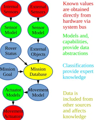
In a Bayesian network representation, everything the rover knows is rep-resented as linked random variables. The knowledge (priors, etc.) is initially provided by the rover’s self-aware devices. Abstractions that need to be in-ferred are provided by the mission plan. Using the communications system detailed above, known values are obtained directly from hardware via the system bus, with models, capabilities, and links between the nodes provided by devices themselves. Abstractions such as the definitions of obstacles and mapped areas of interest are expert knowledge that is typically included in the mission planning data. Figure 6 shows a simple example of a Bayesian network constructed in this manner.

3.4. Node Types

While all nodes in the Bayesian network we construct represent random variables, the variables represent a variety of different real abstractions, and are consequently constructed using different data sources and roles within the Bayesian network. All nodes are kept as similar as possible in terms of data representation and programming interface, and all effectively function as probability distributions over random variables, although data nodes in particular usually call external sources to calculate appropriate responses to queries in real time.

Figure 6: A General Bayesian Network Illustrating Dependencies and Node Types

also be implemented as probabilistic algebraic functions, such as the sensor model for the infrared range sensors. They are usually a parent or child of a bus node. Ability nodes for sensors are typically included

in the set of knowns Kn and ability nodes for actuators are typically

searched in the set Seto make decisions about actuator movement and

operational functions.

• Bus or (B) nodes include hardware devices connected to the system

bus such as the obstacle sensors, inertial sensors, environmental sen-sors, and actuator drivers. Sensor nodes usually are parent nodes only that provide actual measurement values to ability nodes, while actuator nodes are usually child nodes only that are dependent on ability nodes representing their actual function, and have joint distributions repre-senting a “question” regarding the actuator state. A bus node acts as a “terminal” or “endpoint” in the network that allows interaction with the rover itself and the outside world, and generally is associated with

• Classification or (C) nodes are used to interpret and translate infor-mation within the network. For example, an inertial sensor can only give information about probability of body orientation and an obstacle sensor about the probability of the presence of an obstacle, but deter-mining the likelihood of the rover tipping over or the likelihood of a collision are conditional judgments based on inference. Classification nodes act as drivers in determining behaviours to respond to external or internal events, and are most similar to the BRP concept of “Para-metric Forms”. Classification nodes are also generally included in the

set of unknowns Un.

• Data or (D) nodes act as an interface to additional information outside

the network. These include probability maps built as two or three-dimensional distributions, and mission information databases used to build probability distributions dynamically based on external instruc-tions. Data nodes typically use function pointers to refer queries to functions that provide the appropriate information based on the sys-tem state, and are similar to the BRP concept of “Program Forms”. As they provide data, they are usually included in the set of knowns

Kn.

In Figures 6 and 8, ability nodes are coloured green, bus nodes are coloured red, classification nodes are colored blue, and data nodes are colored yellow. Learned probability data is stored and shared in XML format. There have been several different proposed Bayesian Network Interchange Formats (BNIF) developed, such as BIF, XMLBIF, and XBN [26]. Despite a lack of current information and limited scope of adoption, the XBN standard is the most current, although the earlier XMLBIF format appears more efficient to parse. Both formats can currently be used for storage, with additional XML tags implemented to support complete storage of the node structure such as

node type _{A, B, C, D_}.

4. Experiments

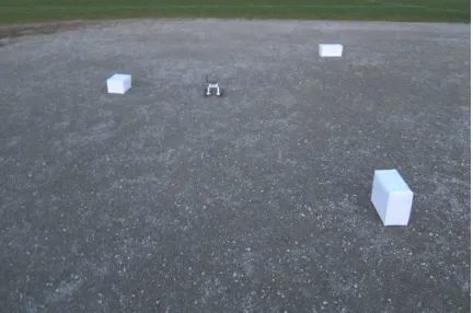
proba-Figure 7: Beaverµrover Prototype in Outdoor Test Area with Obstacles

bilistic models to the sensor and mapping hardware on the µrover and allow

it to map a small area of outdoor space with known obstacles using only the infrared range sensors for obstacle detection. The area mapped by the

µrover is shown in Figure 7. It is open except for three boxes, which due to

the low sensitivity of the infrared sensors are covered with white paper for high reflectivity. In this test, time-averaged GPS is used for coarse position sensing.

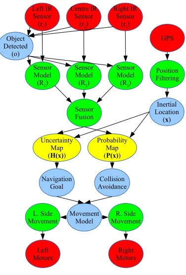
infer the likelihood of object presence at a given location on the map, struc-tured as a Bayesian network to simplify design and calculation. In addition, the uncertainty in the measurement made is estimated, mapped, and used to drive the search methodology. A set of behaviours is then applied to the likelihood map to implement obstacle avoidance. To evaluate performance in a real-world scenario, this system is implemented on a small micro-rover pro-totype and tested in an outdoor area with obstacles present. The Bayesian

network structure used to relate the various aspects of µrover operation for

the mapping task is shown in Figure 8. An early version of this mapping methodology was tested using a simpler monolithic decision-making algo-rithm and without using a the Bayesian network [27] and this was used as a reference for development of the current network of variables, which offers better probabilistic performance, and more importantly, vastly more flexible programmability.

4.1. Range Sensor Model

For the purposes of this study, the rover is tasked to observe all objects

encountered and statistically identify obstacles. The µrover’s infrared range

sensors are used to detect objects based on infrared light reflected from their

surfaces, and each provide a range observation measurement r. Each sensor

model is considered to be of a Bernoulli type with a probability of correct

object detection βr, a fourth-order polynomial function of the range sensor

state, modelled as a random variable R, where [28]

R=_||x₋x¯_{|| ∈R}+ (30)

with ¯xbeing the rover’s estimated current location andxbeing the location

of a sensed object. We can quantify the the probability βr that the range

sensor state R is correct by defining it as

βr = (

βb+ _r1_max−βb4(rmax2−R2)2, if R≤rmax

βb, if R > rmax

(31)

where βb is the base likelihood of correct object detection, assumed to be

βb = 0.5 so that an even likelihood of correctness is assumed if the object

is outside the sensor’s range since no actual information of object presence

will be provided to the sensor. rmax is the sensor’s maximum range of

ap-proximately 2m, beyond which correct and incorrect object detection are

at ¯x is 1 (certainty) and occurs closest to the sensor, which generally has higher accuracy when closer to an object. This provides a model by which

the assumption of object presence at R can be made based on the actual

measurement of r.

A probabilistic method is used to update the probability of object

pres-ence given a range observationr. We define the likelihood of an object being

present at range R from the current location and time t+ 1 given the range

observations r as P(R_|r, t+ 1) and taking into account the reliability of the

sensor. Although we have no other reference for object detection besides the range sensors, we can increase accuracy by including any knowledge we have

already regarding object presence at a given map locationxwith the variable

o =_{0,1_} with 1 defining an object being present and 0 defining an object

not being present. This can be written in the form P(R_|r, o, t+ 1), which can

be solved for by applying Bayes’ rule as [29]

P(R_|r, o, t+ 1) = P(r|R, t)P(R, t)

P(r, t) (32)

=

( _βrP(R,t)

2βrP(R,t)−βr−P(R,t)+1, if o= 1

(1−βr)P(R,t)

−2βrP(R,t)+βr+P(R,t), if o= 0

where we use the law of total probability and the fact that P(r_|R, t) is given

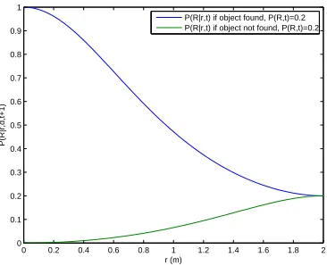
by βr. Equation 32 represents the “Sensor Model” nodes in the Bayesian

network of Figure 8. This probability distribution is shown for the case

where the probability of object detection by itself is constant as P(R, t) =

P(R) = 0.2 in Figure 9. Of note is the fact that regardless of object detection

o, the distribution converges to P(R, t) at r =rmax. To determine whether

an object has been contacted, we need to make sure the output of the range sensor is above the noise level of the device, for which we make sure at least

two samples in a row indicate that contact well above the RMS error σr is

made.

o= (

1, ifrraw(t)>2σr∧ rraw(t−1)>2σr

0, otherwise (33)

4.2. Range Sensor Fusion

Three directional infrared sensors are placed on the front of the rover for

0 0.2 0.4 0.6 0.8 1 1.2 1.4 1.6 1.8 2 0

0.1 0.2 0.3 0.4 0.5 0.6 0.7 0.8 0.9 1

r (m)

P(R|r,d,t+1)

P(R|r,t) if object found, P(R,t)=0.2 P(R|r,t) if object not found, P(R,t)=0.2

Figure 9: Probability Distributions P(R|r, d, t+ 1) for Infrared Range Sensor Model

sensor. To improve the detection reliability of objects in the probability map, the sensor data is combined using a linear opinion pool. Each sensor set at

an angle θr is assumed to have a sensor angle of view wr and a Gaussian

horizontal detection likelihood, so the detection probability incorporating angular deviation for each sensor is estimated as

αs= 1

w2

r √

2π ∗e

−(_wrθr)2

. (34)

To combine probability information in the Bayesian network, we can cre-ate a node that depends on other nodes above it in the structure. To combine the information from the three sensors together, we use the “Sensor Fusion”

node, which provides an opinion pool forN sensors at angles ofθn, n= 1. . . N

with respect to a primary direction by

P(R_|r, o, t, θ1, θ2,· · ·θN) (35)

= N X

n=1

P(R_|r, o, t)_∗ 1

w2

r √

2π ∗e

−(_wrθn)2

.

4.3. Map Updates

Mapping of object probabilities is done at each pointxwithin the sensor

range rmax of ¯x at the angle θr. The rover’s map is structured as an

distribution over obstacle presence O. Initially, every grid element in the

map is initialized to P(R), the estimated probability of encountering an

ob-stacle in this environment, and the map is updated at the locations pointed to by the sensors. We consider map updates to be a Bayesian parameter es-timation problem using a joint probabilistic model to obtain the probability

P(O_|R,x, t) of an obstacle being present at x. We use the estimate of the

probability of a range measurement given an obstacle atx, the probability of

an obstacle P(O,x, t), and the prior for any obstacle detection with Bayes’

rule to form

P(O_|R,x, t+ 1) = P(R|O,x, t)P(O,x, t)

P(R,x, t) . (36)

A two-dimensional Gaussian function can be used to estimate P(O_|R,x, t+

1) on the map to capture the uncertainty in positional measurement. While the main goal is statistical identification of obstacles, it is also important to know how much certainty is present at each point in the map. The un-certainty in a measurement can be modelled as the informational entropy

present [30]. The information entropy at x and time t for a Bernoulli

distri-bution Ps={Ps,1−Ps} are calculated as

H(O_|R,x, t+ 1) (37)

= min

t (−P(R,x, t) ln(P(R,x, t))

−(1₋P(R,x, t)) ln(1₋P(R,x, t))).

The minimum of all measurements over t taken at a mapped point x

is used to reinforce that uncertainty decreases over time as more data is gathered. The use of a probabilistic sensor model allows the rover’s view of the world to be fuzzy, so that rather than assuming a precise location for obstacles and landmarks, the rover can choose the path that is least likely to contain obstacles, and also consider the locations on the map that contain the least information to be the least reliable. This makes the system more robust to position errors and sensor inaccuracies, as it will attempt to choose the best solution while considering the presence of statistical errors such as Gaussian noise.

The rover maintains two maps of its operating area, one for detected

which are constant over t unless sensory data is added at any point x. As the rover is currently only intended to travel several meters to carry out a mission goal, this is sufficient for short-range travel. The “Probability Map” node provides an interface from the occupancy grid to the Bayesian network by representing the map as a two-dimensional discrete probability distribution. As a probability distribution, the map can be part of a query to obtain the probability of obstacles at a specific location, or updated as part of a learning process with the original map serving as the prior distribution. The main difference in considering the map a probability distribution is that each row or column must be normalized to the size of the map for queries to be accurately carried out.

4.4. Mapping Methodology

Assuming the rover is present at the centroid of a grid element ¯x then a

sensor reading at range rwill affect positions P(xx+rcos(θr),xy+rsin(θr))

and any adjacent locations within the distribution spread of the sensor.

En-tropy is mapped in much the same way, as H(xx+rcos(θr),xy+rsin(θr)) for

orthogonal Cartesian components xx and xy for each θr. Before any data is

gathered, the probability map is initialized to P(R), while the entropy map

is normally initialized to 1 at every point. As the search process within the map is not generally randomized, this leads to the same pattern being re-peated initially. To evaluate the impact of varying initial uncertainty on the search pattern, the entropy map was also initialized using a pseudo-random

value δh <1 as 1−δh < H(x) <1 in a separate set of tests. For efficiency,

the rover is assumed to only evaluate a local area of radius dmax in its stored

map at any given time t. Mapping continues until there are no remaining

points with uncertainty exceeding a given threshold, (_∀x,H(x)< Hdesired).

Considering the set ∆s as all points within this radius, where {∀x ∈

∆s,||x−x¯|| < dmax}, the target location ˆx is generally chosen to be the point with maximum uncertainty:

ˆ

x′ _{= arg max}

∆s

(H(O_|R, r,x)). (38)

However, as this typically results in mapping behaviour that follows the numerical map search algorithm, it is desirable to provide a more optimal search metric. We choose the map location with maximum uncertainty within

the margin δh and minimum distance from the rover and use a logical OR

ˆ

x= ˆx′ _{∨[arg max}

∆s

(H(O_|R, r,x)₋δh)∧arg min

∆s ||

x₋¯x_||]. (39)

To make the target destination available as a probability distribution, we use a maximum likelihood estimation process to create a Gaussian

distribu-tion over a target locadistribu-tion random variableT with the mean at the horizontal

angle θt aiming toward ˆxand with a standard deviation ofπ radians so that

at least a 180◦ _{arc has probability of reaching the target.}

P(T_|R,d, θt) =

1 π

2

√

2πe

−(x−θ)2

π2/4 (40)

The node “Navigation Goal” in Figure 8 encapsulates this so that queries can be performed. The spread of the Gaussian distribution allows a wide variety of choices for steering angle even if obstacles are present between the rover and the target.

4.5. Navigational Decisions

For forward navigation, we would like to travel to the target location by the shortest route possible while minimizing the risk of a collision. From a naive Bayes standpoint, what we need is a probability distribution that includes both the probability of collision across the possible steering angles of the rover, and the distance to potential obstacles so that closer obstacles count as more dangerous than distant ones. This can accomplished by first

obtaining the vector d = ˆx′ _{−x¯ from the rover to the target point, and}

considering the area of the map occupying the solid angle θdfrom this vector

centred on the rover, such that the angles θ _∈ [₋θd. . . θd] with respect to

d are considered. A set of M discrete angles θm, m = 1. . . M can then

be evaluated by summing the normalized total probability of encountering

an obstacle over all locations along the length dmax vector xθ to form the

probability distribution

P(O_|R,d, θm) =

P

xθP(O|R,xθ)

dmax

. (41)

This provides a metric for the likelihood of encountering an obstacle in

the direction θ and allows existing map data to help plan routes. To

incor-porate the concept of distance, the sum of the distribution is weighted by the

distance _|xθ−x¯|, effectively increasing the likelihood of encountering closer

P(O_|R,d, θm) = P

xθ(dmax− |xθ−x¯|)P(O|R, r,xθ)

dmax

(42)

The probability distribution P(O_|R, r, d, θm) is implemented in the

“Col-lision Avoidance” node in Figure 8, and is used together with the target location to drive the “Movement Model” node, which calculates a

distribu-tion P(M_|O, R, r,d) over a random variable of movement direction M to

prioritize the target point, but avoid areas with high obstacle likelihood.

P(M_|O, R,d) = P(T_|R,d, θt) + (1−P(O|R,d, θm)) (43)

The query arg max

M P(M|O, R, r,d) is then used to determine the best choice of direction for forward movement.

5. Results and Discussion

The Beaver was given a 20m by 20m area for motion, and mapping was constrained to this area in software, although the rover could physically leave the map due to turning radius constraints. Using the Bayesian mapping strategy with the goal of exploring all the given map area thoroughly, the rover was allowed to move freely in an area with no obstacles. For this test,

βb = 0.2, dmax = 8m, P(R) = 0.2, and a grid with 0.5m resolution were

used. The grid resolution reflects not only the noise and uncertainty in GPS measurements, but also the safety margin around obstacles that is desired to avoid collisions.

5.1. Range Sensor Characterization

To evaluate the performance of theµrover infrared range sensors used for

navigation, the µrover was placed at 2m from one of the mapping obstacles

and driven forward while taking positional measurements. By driving the

infrared emitter with its maximum design voltage of 7V, a maximum range

ofrmax= 2mis possible, which is assumed by the sensor model. Additionally,

to ensure that the range sensor would function at oblique angles to a target,

a mapping obstacle was placed at 1m distance and the normal of the facing

surface rotated through ϑo = (45◦. . .−45◦) with respect to the line of sight

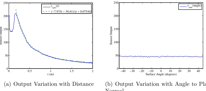
of the sensor. Profiles of digital range rraw versus actual range and digital

range with respect to the facing surface angle of the target ϑo are plotted in

0 0.5 1 1.5 2 0

50 100 150 200 250

r (m)

Sensor Output

r raw(r)

(−7.933r + 56.61)/(r + 0.07544)

(a) Output Variation with Distance

−40 −30 −20 −10 0 10 20 30 40 0

50 100 150 200 250

Surface Angle (degrees)

Sensor Output

r raw(angle)

(b) Output Variation with Angle to Plane Normal

Figure 10: Infrared Range Sensor Profiles for Distance (a) and Angle (b)

An 8-bit ADC is used for measurement of the range sensor, and the

sensor output noise level remains within _±1 8-bit unit throughout most of

the test. Fitting the profile of rraw to a first-order rational function yields

the polynomial fit rraw ≈(−7.933r+ 56.61)/(r+ 0.07544), which is solved for

r to obtain the transfer functionr=₋(0.08(943rraw−707625))/(1000rraw+

7933) used to calculate the actual range from the given measurements. The combination of sensor, ADC, and polynomial fit noise results in an RMS

error ofσr = 2.777 8-bit units (1.33%) inrraw, which is more than acceptable

for the main driver of uncertainty in the map, our rover positioning error.

Variation with target surface angle of rraw(ϑo) is also very low, showing no

appreciable dependence on ϑo and only slightly higher noise than with no

rotation. As there is no fitting estimation, an RMS error of 1.015 is observed

0 5 10 15 20 0 2 4 6 8 10 12 14 16 18 20 Probability Map 0 0.1 0.2 0.3 0.4 0.5 0.6 0.7 0.8 0.9 1

(a) P(O|R, r,x)

0 5 10 15 20 0 2 4 6 8 10 12 14 16 18 20 Uncertainty Map 0 0.1 0.2 0.3 0.4 0.5 0.6 0.7 0.8 0.9 1

(b) H(O|R, r,x)

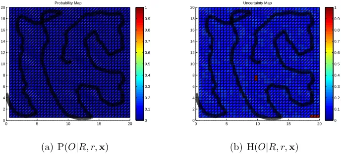
Figure 11: Probability and Uncertainty Maps Found by µrover, No Obstacles

5.2. Autonomous Mapping Without Obstacles

First, each location in the probability map was initialized to 0 and each in the entropy map was initialized to 1. Figure 11 shows the probability and uncertainty maps. The path that the rover took during the test is shown as an overlaid black line. The initial entropy map was then modified with

a pseudo-random offset as suggested above with δh = 0.1. Figure 12 shows

the probability and uncertainty maps. The new path that the rover chose is shown.

5.3. Autonomous Mapping With Obstacles

Three obstacles were then placed in the 20m by 20m area to test the

obsta-cle avoidance methodology. Two 1mx1mobstacles were placed at (14m,16m)

and (7m,10m), and a 0.5mx1m obstacle was placed at (12.5m,3m) in grid

coordinates. The layout of the testing area used is shown in Figure 7. The rover was run with the same parameters as the tests above with the un-certainty map initialized to 0 and the entropy map initialized to 1. The resulting path and maps are shown in Figure 13. The test was repeated with

the pseudo-random offset as suggested above with δh = 0.1, and the results

are shown in Figure 14.

The obstacles are not overly obvious given the statistical nature of the mapping, but they are visible as points of high probability and low uncer-tainty, while the remainder of the mapped area retains an uncertainty of close

0 5 10 15 20 0 2 4 6 8 10 12 14 16 18 20 Probability Map 0 0.1 0.2 0.3 0.4 0.5 0.6 0.7 0.8 0.9 1

(a) P(O|R, r,x)

0 5 10 15 20 0 2 4 6 8 10 12 14 16 18 20 Uncertainty Map 0 0.1 0.2 0.3 0.4 0.5 0.6 0.7 0.8 0.9 1

(b) H(O|R, r,x)

Figure 12: µrover Probability and Initially-Randomized Uncertainty Maps Found by

µrover, No Obstacles

0 5 10 15 20 0 2 4 6 8 10 12 14 16 18 20 Probability Map 0 0.1 0.2 0.3 0.4 0.5 0.6 0.7 0.8 0.9 1

(a) P(O_|R, r,x)

0 5 10 15 20 0 2 4 6 8 10 12 14 16 18 20 Uncertainty Map 0 0.1 0.2 0.3 0.4 0.5 0.6 0.7 0.8 0.9 1

(b) H(O_|R, r,x)

0 5 10 15 20 0 2 4 6 8 10 12 14 16 18 20 Probability Map 0 0.1 0.2 0.3 0.4 0.5 0.6 0.7 0.8 0.9 1

(a) P(O|R, r,x)

0 5 10 15 20 0 2 4 6 8 10 12 14 16 18 20 Uncertainty Map 0 0.1 0.2 0.3 0.4 0.5 0.6 0.7 0.8 0.9 1

(b) H(O|R, r,x)

Figure 14: Probability and Initially-Randomized Uncertainty Maps Found byµrover, With Obstacles

to small differences in location xor sensor reading r that occur due to