City, University of London Institutional Repository
Citation
: Sastuba, M., Skupsch, C. and Bruecker, C. ORCID: 0000-0001-5834-3020
(2014). Real time visualization and analysis of sensory hair arrays using fast imageprocessing and proper orthogonal decomposition. Paper presented at the 17th International Symposium on Applications of Laser and Imaging Techniques to Fluid Mechanics, 7-10 July 2014, Lisbon, Portugal.
This is the accepted version of the paper.
This version of the publication may differ from the final published
version.
Permanent repository link:
http://openaccess.city.ac.uk/21392/Link to published version
:
Copyright and reuse:
City Research Online aims to make research
outputs of City, University of London available to a wider audience.
Copyright and Moral Rights remain with the author(s) and/or copyright
holders. URLs from City Research Online may be freely distributed and
linked to.
City Research Online: http://openaccess.city.ac.uk/ [email protected]
Real time visualization and analysis of sensory hair arrays using fast
image processing and proper orthogonal decomposition
Mark Sastuba
1,*, Christoph Skupsch
2, Christoph Brücker
11: Institute of Mechanics and Fluid Dynamics, University of Freiberg, Freiberg, Germany 2: Frauenhofer-Instiut für Photonische Mikrosysteme IPMS, Dresden, Germany
* correspondent author: [email protected]
Abstract This paper presents an approach both to receiving multiple sensor data from a flow in real time and to
analyzing these data in order to characterize the flow condition and, if necessary, control the flow. In order to obtain the data, an optical micro-pillar array acting as distributed wall-shear sensor was developed and interrogated optically with an LDM (long distance microscope). Together, the micro-pillar array and the LDM form a channeling optics, which allows magnified imaging of larger numbers of individual pillars simultaneously. The sensor was tested in a turbulent wall shear stress field under varying conditions (Reynolds number). A frame rate of 3000 fps was used since the higher the temporal resolution is, the more specific flow control strategies might be applied later in realistic application. However, the temporal high resolution would lead to a vast amount of data, which is difficult to analyze in real time. Therefore, a fast image processing algorithm is developed, which detects the tip deflections of the pillars and vectorizes the wall-shear stress field online. The extracted data fields are then broken down into equidistant and overlapping windows in order to guarantee fast POD (proper orthogonal decomposition) modes calculation. The POD is applied to each of these windows and the extracted modes are compared, summarized and collected in a library. Finally, this library is again applied to the flow but under different conditions in order to identify the state of the current flow in real time.
1. Introduction
Real time flow observation close to the wall is still a challenging process, when it comes to detect flow separation or transition under highly unsteady conditions. A promising technique is the use of flexible micro-pillars to detect the wall-shear stress field [1,2,5]. Due to the drastic performance increase of computational power, direct analyses – even with small delay – have moved into the scope of practical implementation. The possibilities of direct investigation as well as the possible forecast of critical flow conditions establish the basis for new methods of live flow control (investigation).
In the first part, this paper describes a real time image analysis approach of an unsteady wall shear stress field by using Matlab’s built-in processing routines. An optically interrogated micro-pillar array sensor field is used to capture 21 scattered wall-shear vectors in a flow field. The sensory hairs are fully submerged in the viscous sublayer of a turbulent wall jet and serve as wall-shear stress sensors. The main goal is to identify from these hair motions dominant structures that specify the flow characteristics by means of the observed deflection data of the pillar tips. Furthermore, the presented algorithm reduces the data amount dramatically. Instead of saving image data for each time step, only 21 vectors (parallel x- and y-direction of the wall-shear stress vector of each pillar) are processed and stored.
The second part of this paper describes a real time POD (Proper Orthogonal Decomposition) approach which is applied to the pillar data. The focus concentrates on the extraction of dominant flow features in real time in order to characterize the underlying dynamics.
All presented benchmark tests were performed on the same computer with the following technical specifications. Processor: Intel Core i7 3930K (6 physical cores at 3,2 GHz), Graphics: Nvidia GeForce GTX
2. Experimental Setup
The experiment uses an optically interrogated micro-pillar array sensor, which, compared to other sensors, influences the flow less [5]. The recently improved design of the sensor imaging contains a LDM (Long Distance Microscope), an extension lens and an aperture array. This combination is called channeling LDM and is shown in Figure 1. The main benefit is that each micro-pillar is imaged through its own optical channel. This allows to decompose the field of view into single sections and to magnify distributed regions of interest, whereas the whole micro-pillar array would not fit on the camera chip at the same magnification level.
In [5], the authors describe the installation of the optical pillar array sensor, define its properties and apply the sensor to an unsteady wall shear stress field. As a further step towards a flow control unit using such sensor concepts, the present paper focuses on the fast detection of the pillar tip deflections quasi on-line while recording. Afterwards, a POD is applied to the covered data in order to extract significant flow structures [6]. Furthermore, the influence of noise, which is caused mainly by inaccurate center detection of the pillars, is analyzed.
Figure 1: left: schematic drawing of the channeling long distance microscope (LDM) to magnify regions (pillars) of
interest [5], right: applied channeling LDM in an experimental setup for wall shear stress measurements [5]
In [5], flow observations were performed under different Reynolds numbers at a constant capturing frame rate of 3000 fps. These image data are used in this paper again and hold as the data space. The developed algorithm is applied to two time series (2048 images each), which were captured under Re = 1090 and Re = 1290. The resulting data throughput is determined afterwards.
The use of a high frame rate allows measuring all dynamical aspects of the observed flow, which are necessary for the analytical step and structure identification. Although the algorithm is not able to handle the current frame rate in real time, it is used to evaluate and improve the processing speed. The image sequence
represents a basic data set for the benchmark. Nevertheless, recent progress in FPGA (Field Programmable
Gate Arrays) in combination with high-speed cameras may allow running the software described herein for higher frame rates as well.
3. Methods of fast pillar detection
[image:3.595.99.506.298.465.2]MatLab provides a wide range of image processing algorithms and additional ones to find specified shaped geometries (in this case circles) [3]. However, during previous tests, the used detection algorithms tended to fail at higher pillar deflections due to blurring caused by the bending of the pillar shaft. Furthermore, a clear loss of speed performance was noticeable, too. Consequently, a simple but robust cross-correlation was chosen to detect the centroids of the pillars.
a b
c d
Figure 2: Image processing steps for calibration, (a) captured image (grey scaled), (b) mask of detected lens array
(black-white), (c) lenses registration 1-21, visualization of their edges (yellow) and perimeters (dotted blue) highlighting the area of investigation for cross-correlation, (d) detected pillar centroids of zero deflection (green cross)
Therefore, each lens cutout is edited separately to highlight the pillar shape in order to achieve good correlation results. The sequence of applied image filters is presented in Figure 3 (a)-(d).
[image:4.595.126.477.161.518.2]a b c d e
Figure 3: Image editing process of one pillar, (a) original image (gray scaled) showing the shape of the pillar from top,
(b) applied image filter and masking, (c) inverted image, (d) image with applied edge detection filter, (e) sample of an ideal micro-pillar shape with highlighted centroid spot (green cross)
[image:4.595.114.484.616.687.2]the filtered micro-pillar image.
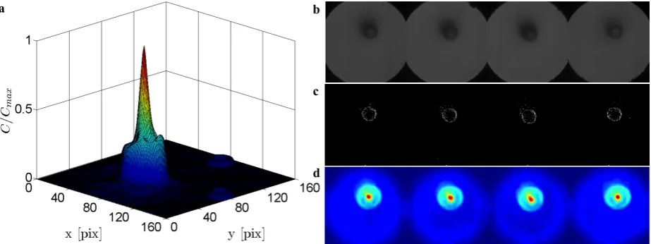
The resulting 2d-correlation distribution is visualized in Figure 4 (a) and shows a clear peak, which indicates the position of the best fit. By means of that, the center point of the sample is shifted to obtain the micro-pillar position of zero deflection in the calibration. This routine is repeated for all 21 lenses.
c b a
[image:5.595.69.531.151.324.2]d
Figure 4: (a) Result of the normalized 2d cross-correlation between micro-pillar sample and one filtered pillar image,
peak indicates best matching position (shift), (b)-(d) overview of 4 out of 21 stringed lens cutouts, (b) original, (c) image filtered, edges highlighted, (d) results of cross-correlation, peaks clearly visible (red spots)
For a proposed analysis at real time frame rate, this process has to be improved in order to reduce computational effort. The lens cutouts – each with the same dimensions – are stringed together to form a new image as shown in Figure 4 (b). All image filters as well as the cross-correlation are applied to this particular new image as shown in Figure 4 (c) and (d). This procedure prevents the use of loops. Instead of computing 21 small data files, only one data file, yet 21-times bigger in memory, is processed.
The main advantage of this method becomes obvious when cross-correlation is done by the GPU. For that
purpose, the image data has to be transferred from the computer memory to the memory of the GPU. By reducing the number of transfers, the operation becomes faster. However, depending on the data size of the image and the limited memory size of the GPU, the cross-correlation is not always executable in this way. After cross-correlation, a peak search is performed for each sector of a lens cutout to obtain the shift and to calculate the corresponding center position of a particular micro-pillar.
4. Results of fast image processing
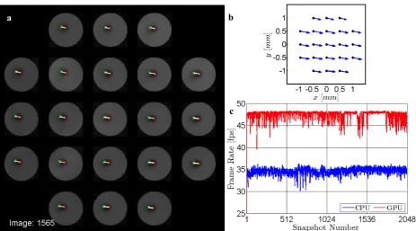
The following Figure 5 (a) presents an example of the original image footage at Re = 1290 with visualized
detection results as well as the corresponding vector plot in Figure 5 (b).
a b
c
Figure 5: (a) Example of pillar detection including pillar centroids (red dots) and calibration positions of zero
deflection (green crosses), (b) plot of corresponding vector field, (c) comparison of micro-pillar detection between CPU
and GPU, average CPU-frame rate 34.6 fps, average GPU-frame rate 47.3 fps
5. Analysis of signal quality
This section focuses on the influence of noisy data on proper orthogonal decomposition. The POD-analysis
is performed as a separate or post-processing operation, due to the limited CPU-performance. As already mentioned, the above-described algorithm is suitable for fast image processing to detect relevant data, which requires an adequate signal quality. Furthermore, it is necessary to investigate the influences of disturbed signals on the decomposition process. The main and most important source of erroneous data is the pillar detection which tends to be inaccurate in some cases, especially at high pillar deflections caused by intensified blurring at the pillar shaft. Also, relative motion caused by vibrations of the pillar field, the lens array or the camera itself influence the detection quality. All of those might be improved by detection of reference points on the wall and coating of the pillar tips with reflective material.
In order to evaluate the POD-decomposition based on varying signal quality, the original data sequence KO is smoothed by a moving average filter (MAF) to get a new signal KS, which is supposed to contain fewer disturbances. It is assumed that the larger the span of MAF, the better the signal quality, however, the reproduction of fluctuations decreases. This leads to an optimization problem of finding a threshold to distinguish disturbances (noise) from fluctuations.
The data sequence K is constructed by
{
}
11 /2, 1 /2
T M
j M M
u dx dx dy dy ×
= L L ∈£
,
(1)
which is a column vector containing the detected pillar deflections dx and dy at a specific time step j. In this case the dimension of observables M is 42. All snapshots of the time series are stacked such that follows
[
1, ,]
M N NK u u ×
= K ∈£
,
(2)
[image:6.595.67.531.68.325.2]( )
(
)
( )
( )
(
)
2 1 1 10 2 1 1 1 , 10log 1 , , M N S i j M N O S i jK i j MN
S
K i j K i j MN = = = = ⎛ ⎞ ⎜ ⎟ ⎜ ⎟ = ⎜ ⎟ − ⎜ ⎟ ⎝ ⎠
∑∑
∑∑
.
(3)
Next, different interpolation spans MAF = 1...201 are used to obtain a smoothed signal in order to determine S. Please note that this equation is analog to the calculation of the signal to noise ratio (SNR) but it does not mean the same. Here, it is used as a tool to locate the initial limits of the MAF. To identify the influence of MAF on S the partial differential
∂ ∂
S MAF
is calculated as shown in Figure 6 (a). The red line highlights the point, were the slope of the curve becomes quite linear. This point indicates the upper limit for a smoothing interpolation with MAF = 51, which stands for best signal quality. Figure 6 (b) shows an example of covered deflections of one pillar and the resulting smoothed signal with MAF = 51.a
[image:7.595.89.507.260.415.2]b a
Figure 6: (a) Signal level over interpolation span of MAF, red dotted line indicates upper limit of interpolation span, (b)
example of covered pillar deflection (blue) and its smoothed signal (red) with MAF = 51
6. Proper orthogonal decomposition and mode correlation
In the next step, the POD is applied to the original data sequence KO and the smoothed one KS (MAF = 51) in order to see the maximum influence of the filtering on the decomposition. In fluid dynamics, the POD is used to extract dominant flow characteristics by identifying coherent structures. Therefore, the mean data field 1 1 N i i u u N = =
∑
%(4)
is subtracted from each snapshot to achieve a time series of fluctuations
[
1 , ,]
M N N
K u u u u ×
= − − ∈
% %K % £
(5)
to which the decomposition is applied. Therefore, the covariance matrix C is calculated by the following equation
T N N
C K K ×
= % % ∈
.
(6)
The eigendecomposition of C leads to the eigenvectors µ and eigenvalues λas described by
Finally, the normalized POD-modes are calculated as follows
1
1
M N N
N
K µ µ
φ
λ λ
×
⎡ ⎤
= ⎢ ⎥ ∈
⎢ ⎥
⎣ ⎦
% L
.
(8)
The results of the most energetic modes of the applied POD-algorithm as well as the mean data field are shown in Figure 7. It is obvious that the shapes of the modes are nearly identical.
Figure 7: POD-results of the first three modes and the mean data field (Mode0) of the original data sequence and the
smoothed one, the numbers in brackets indicates the energy of the smoothed data, ρ denotes the correlation coefficient between original and smoothed data
In order to quantify the matching, a correlation coefficientρis introduced
,
i j
i j
i j
φ φ ρ
φ φ
= o
,
(9)
[image:8.595.118.482.211.595.2]The correlation can only be performed with normalized modes, yet the standard POD-algorithm generates orthogonal structures. Thereby the equation is simplified to
,
i j i j
ρ
=φ φ
o.
(10)
Furthermore, in case of correlating two POD-modes where ρi,j = -1, both modes describe the same orthogonal structure, however, they are in opposite direction. This statement is based on the fact that each POD-mode Φ is multiplied by a corresponding time dependent weighting factor α(t) (chrono) in order to recalculate the original data field. Thus, ifρi,j = -1, then αi(t) = -αj(t), which can be brought into the following
context
( ) ( )
i t i j t j
α
φ
=α
φ
.
(11)
By means of Figure 7, it is recognizable that the higher the energy of a mode, the better the correlation. The total sum of fluctuation energy for the three modes is 95,3% for the original and 98,3% for the smoothed case, which is a negligible difference of approximately 3%. Also, the energy distribution is remarkable. The main fluctuation energy is contained in the first and second POD-mode, whereas the third one contains only a small portion. Mode0 defines the mean data field and contains no fluctuation energy. However, it is also necessary to investigate the correlation of these data structures since they determine the sequence of fluctuations and by means of that, the POD-modes.
Based on these results, with an MAF = 51 it is possible to smooth the data without changing the structures (modes), which are responsible for the majority of energy content of the whole data sequence. The POD -algorithm ranks the structures according to their energy content, that is, this value demonstrates the occurrence of each mode in the data ensemble. In order to reduce the influence of noise, it is recommended to compare “higher” energetic modes [4]. Unfortunately, there is no fixed value for that. It depends on the dynamic data and the resulting energy distribution of the decomposition process. In the case presented here, mode one and two describe the main fluctuations. These modes show the best matching results since they are obviously not affected by noise. The smaller the energy content of a mode, the more it is influenced by disturbance and therefore not comparable. For a decomposition with a window size of N = 2048 (whole snapshot sequence), there are no notable differences in the identified structures of KO and KS.
7. Sliding window base analysis
As already mentioned, a real time POD is aimed at. Unfortunately, it turned out that the window size (number of snapshots), which the POD is applied to takes too long to handle the data amount in an adequate time interval. The idea is to reduce the window size and to make the window moveable. This means that instead of applying the POD to the whole sequence at once, the sequence is split into equidistant and overlapping time intervals (windows) on which the actual analyzing process is performed. After the analysis of the current window is finished, the window slides one time step forward, the analysis starts again and the identified structures are compared.
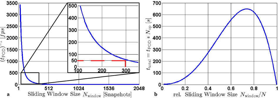
considers the processing power of the computer. The more snapshots are observed by POD, the larger the data matrices become which reduces the calculation speed immensely. Figure 8 (a) demonstrates the dependency of the POD-calculation time tpod (which is inverted to get the calculation speed in fps) over the sliding window size Nwindow for the used computer. The analysis shows an exponential decrease of the calculation speed. The red line indicates the maximum window size to ensure a calculation speed of 50 fps, which equals the processing speed of the GPU-powered pillar detection. Figure 8 (b) presents the total calculation time ttotal of the POD-analysis over the relative sliding window size Nwindow/N. With increasing Nwindow the number of POD-operations Nop decreases since N is a fixed number. The comparison presented here is only possible if the length of the whole data sequence is known (N = 2048 snapshots). The curve shape is determined by multiplying the POD-calculation time tPOD for a particular window size Nwindow by its number of POD-operations Nop, assuming the window slides one time step forward for each operation.
[image:10.595.63.538.233.401.2]a b
Figure 8: (a) Influence of the window size Nwindow on the POD-calculation time tPOD, red line in magnification cut out
highlights the calculation speed of 50 fps, which is approximately the same as in the pillar detection process (b) total calculation time ttotal (POD-calculation time tPOD multiplied by the number of POD-operations Nop) over the relative sliding windows size Nwindow/N, where N = 2048
The curve behavior indicates the fastest processing speed in range of 0.1*N. The curve reaches the maximum at 0.75*N before it decreases strongly and reaches a minimum at 1*N again. Although the total calculation time at the beginning and ending of the curve seems to be at the same level, the goal is to perform a real time observation that reacts immediately. Furthermore, in practical adaption the sequence length N will be unknown or comparatively infinite.
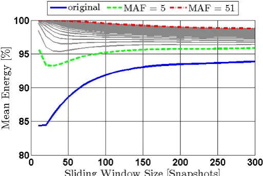
At this point the preliminary considerations lead to the following parameter limitations. The maximum moving average filter MAF = 51 in order to describe a good quality signal (nearly disturbance free signal). The main fluctuation energy (over 90%) is represented by the first three POD-modes and the maximum sliding window size Nwindow = 300. These limitations are used to find the optimal MAF and Nwindow. A new
process calculates the POD-modes by varying MAF = 1…51 and Nwindow = 25…300. The energy contents of
the first three POD-modes are summed up for each window and averaged afterwards. The results are presented in Figure 9.
As a first conclusion for all MAFs, the mean energy becomes more stable, the larger the window size. Starting at a sliding window size Nwindow = 200, the curves become clearly linear. MAF = 5 shows the strongest increase of energy, whereas larger MAF increase the energy level only barely. The value of MAF=5 lies within the range of the strongest influence of the signal (see Figure 6). Please note that MAF = 1 and MAF = 3 do not influence the signal quality and hence they share the same mean energy curve as the original data set KO.
Figure 9: Results of the mean energy distribution against sliding window size and moving average filter (MAF)
8. Decomposition of calibration data and evaluation
The upcoming section describes the analysis of the first data series (Re=1290). The analysis is performed under varying conditions. In a first instance, the sliding window POD is applied to the data sequence under differing signal conditions K1 (signal quality increases). This is called calibration process. In a second step the extracted modes are used to characterize the flow conditions of the same data sequence under similarly varying signal conditions K2. This procedure is called evaluation process. It is done to prevent the following circumstance: a system is calibrated with a special flow phenomenon that is used to observe an unknown flow structure and the same flow phenomenon occurs as in the calibration process. Now the signal quality decreases due to disturbances and the modes will not be identified as a known state.
In the calibration process, all POD-modes with energy higher than 2 % are captured and compared – if available – with prior identified ones in the POD-library. The minimum energy is defined as a threshold in order to distinguish between necessary and negligible modes and orientates on the results of the POD
-decomposition of the whole data sequence. A mode correlates when ρ≥ 0.96, where ρis chosenwith respect
to the former investigations. If ρ≥ 0.96, the mode does not need to be stored. All extracted POD-modes obtained from one signal state of K1 form the POD-library, which is used in the evaluation process to characterize the same data sequence K2 (under different signal quality) again.
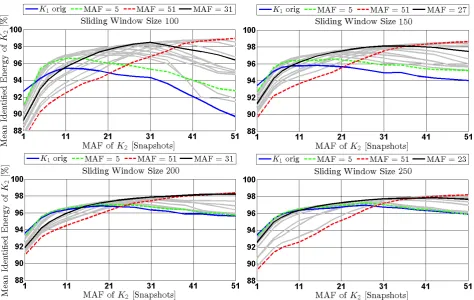
The results of the calibration evaluation can be seen in Figure 10 under four different sliding window sizes 100, 150, 200 and 250 snapshots. For better presentation, the identified energy of each sliding window for one POD-library of K1, which correlates with one sequence of K2, was averaged.
By means of the evaluation it is shown that a minimum of 90 % energy can be identified independently from the degree of disturbance of the signal. The better the signal (high MAF) of both sequences K1 and K2, the better the identified energy. Interestingly, a worse signal of K1 (low MAF), which forms the POD-library, identifies more energy on a good signal of K2 (high MAF) than vice versa (except for sliding window size 100). A black line in Figure 10 highlights the MAF-value of K1 (signal quality) that matches best with all signal states of K2. It should also be mentioned that the range of the mean identified energy for different signal states K1 has a minimum MAF = 23 of K2 for window size 200 and MAF = 29 of K2 for window size
Figure 10: Results of the evaluation process of the calibration showing the mean identified energy of the evaluation sequence K2 over varying signal quality of K2 and calibration sequence K1, black line indicates best signal quality of K1
(in terms of MAF) for correlation, analysis was performed under different sliding window sizes 100 - 250 snapshots
9. Application of identified structures to unknown data sequence
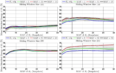
Figure 11: Results of the identification process showing the mean identified energy of the investigated sequence K2
over varying signal quality of K2 and calibration sequence K1, black line indicates best signal quality of K1 (in terms of MAF) for correlation, analysis was performed under different sliding window sizes 100 - 250 snapshots
10. Conclusion and outlook
This paper describes two methods; first, in order to obtain multiple sensor data by applying a new optical sensor and second, in order to analyze these data to characterize dominant features of the observed flow. The
optical sensor consists of a micro-pillar array and a channeling LDM (Long Distance Microscope), which is
used to magnify distributed regions of interest which would not fit on the camera chip at the same magnification level. This paper presents a method to obtain deflections from 21 pillars by using a cross-correlation approach in order to achieve fast image processing.
The developed algorithm is applied to two time series (2048 images each) of an unsteady wall shear stress field, which were captured under Re = 1090 and Re = 1290. Furthermore, a benchmark test of the algorithm was performed on CPU (34,4 fps) and GPU (47,3 fps),where GPU turned out to be faster. However, the GPU-process is slowed down by data transfer of the memory. For future studies, the implementation and
modification of the algorithm on an FPGA (Field Programmable Gate Array) is aimed at. These FPGAs are
designed for fast logical operations. Particularly image processing and cross-correlation, both significant
steps, can be performed well and much faster on an FPGA-board compared to a computer running MatLab.
In this upcoming step, the camera is connected directly to the FPGA-board to guarantee a fast data transfer and to prevent disturbing delays in the processing pipeline. This device combination will allow increasing the presented algorithm up to the projected limit of 500 fps.
[image:13.595.59.539.71.374.2]10. References
[1] Brücker C, Spatz J, Schröder W (2005), Feasability study of wall shear stress imaging using microstructured surfaces with flexible micropillars, Exp. Fluids 39: 464-474
[2] Brücker C, Bauer D and Chaves H (2007): Dynamic response of micro-pillar sensors measuring fluctuating wall-shear-stress, Exp. Fluids 42, 737-749
[3] Case L., and McClain S. (2013), Image analysis to determine the response of passive surface hairs,
51st AIAA Aerospace Science Meeting including the New Horizons Forum and Aerospace
Exposition, 07 – 10 January, 2013, Grapevine, Dallas, Texas
[4] Raben S., Charonko J., and Vlachos P. (2012): Adaptive gappy proper orthogonal decomposition
for particle image velocimetry data reconstruction, Measurement Science and Technology 23, 025303, DOI: 10.1088/0957-0233/23/2/025303
[5] Skupsch C., Klotz T., Chaves H., and Brücker C. (2012): Channelling optics for high quality imaging of sensory hair, Review of Scientific Instruments 83, 045001, DOI: 10.1063/1.3697997
![Figure 1: left: schematic drawing of the channeling long distance microscope (LDM) to magnify regions (pillars) of interest [5], right: applied channeling LDM in an experimental setup for wall shear stress measurements [5]](https://thumb-us.123doks.com/thumbv2/123dok_us/1524982.105066/3.595.99.506.298.465/figure-schematic-channeling-distance-microscope-channeling-experimental-measurements.webp)