MAXIMUM NON-EXTENSIVE ENTROPY BLOCK BOOTSTRAP FOR NON-STATIONARY PROCESSES

(1)

City, University of London Institutional Repository

Citation

: Bergamelli, M., Novotny, J. & Urga, G. (2015). MAXIMUM NON-EXTENSIVE

ENTROPY BLOCK BOOTSTRAP FOR NON-STATIONARY PROCESSES. L'Actualité Economique, 91(1-2), pp. 115-139.

This is the accepted version of the paper.

This version of the publication may differ from the final published

version.

Permanent repository link:

http://openaccess.city.ac.uk/14897/

Link to published version

:

Copyright and reuse:

City Research Online aims to make research

outputs of City, University of London available to a wider audience.

Copyright and Moral Rights remain with the author(s) and/or copyright

holders. URLs from City Research Online may be freely distributed and

linked to.

(2)

Maximum Non-Extensive Entropy Block Bootstrap for

Non-stationary Processes

I

Michele Bergamellia,1_{, Jan Novotn´}_yb,2_{, Giovanni Urga}c,3

a_{Cass Business School, City University London, UK}

b_{Cass Business School, City University London, UK and CERGE-EI, CZ} c_{Cass Business School, City University London, UK and Bergamo University, Italy}

Abstract

In this paper, we propose a novel entropy-based resampling scheme valid for non-stationary

data. In particular, we identify the reason for the failure of the original entropy-based

algorithm of Vinod and L´opez-de Lacalle (2009) to be the perfect rank correlation

be-tween the actual and bootstrapped time series. We propose the Maximum Entropy Block

Bootstrap which preserves the rank correlation locally. Further, we also introduce the

Maximum non-extensive Entropy Block Bootstrap to allow for fat tail behaviour in time

series. Finally, we show the optimal finite sample properties of the proposed methods via

a Monte Carlo analysis where we bootstrap the distribution of the Dickey-Fuller test.

Keywords: Maximum Entropy; Bootstrap; Monte Carlo Simulations.

J.E.L. Classification Numbers: C12, C14, C15, C46, C63.

Current version: 18/10/2014

I_{We wish to thank participants in the 15th OxMetrics Conference (Cass Business School, 4-5}

Septem-ber, 2014), in particular to Guillaume Chevillon for useful comments. Special thanks to Russell Davidson and Lynda Khalaf for very useful comments on a previous version of the paper. We are greatly in debt with the Editor, Marie-Claude Beaulieu, and an anonymous referee for providing us with very insight-ful comments and suggestions that greatly helped to improve the paper. The usual disclaimer applies. Michele Bergamelli acknowledges financial support from the ”PhD Scholarship in Memory of Ana Tim-berlake”, while Jan Novotny acknowledges financial support from the Centre for Econometric Analysis and GA ˇCR grant 14-27047S.

1_{Centre for Econometric Analysis, Faculty of Finance, Cass Business School, City University London,}

106 Bunhill Row, London, EC1Y 8TZ, UK. [email protected], Tel: +44 (0)20 7040 8089, Fax: +44 (0)20 7040 8881.

2_{Centre for Econometric Analysis, Faculty of Finance, Cass Business School, City University London,}

106 Bunhill Row, London, EC1Y 8TZ, UK and CERGE-EI, CZ. [email protected], Tel: +44 (0)20 7040 8089, Fax: +44 (0)20 7040 8881.

(3)

Maximum Non-Extensive Entropy Block Bootstrap

for Non-stationary Processes

In this paper, we propose a novel entropy-based resampling scheme valid for

non-stationary data. In particular, we identify the reason for the failure of the original

entropy-based algorithm of Vinod and L´opez-de Lacalle (2009) to be the perfect rank correlation

between the actual and bootstrapped time series. We propose the Maximum Entropy

Block Bootstrap which preserves the rank correlation locally. Further, we also introduce

the Maximum non-extensive Entropy Block Bootstrap to allow for fat tail behaviour in

time series. Finally, we show the optimal finite sample properties of the proposed methods

via a Monte Carlo analysis where we bootstrap the distribution of the Dickey-Fuller test.

Keywords: Maximum Entropy; Bootstrap; Monte Carlo Simulations.

(4)

1. Introduction

Since the seminal contribution of Efron (1979) for identically and independent

dis-tributed (i.i.d.) data, the bootstrap method has been extended to handle more complex

data structures. In particular, time-series data fail to satisfy the i.i.d. assumption because

both the data distribution might well change over time and the observations are far from

being independent. In order to preserve the dependence structure, K¨unsch (1989)

pro-poses the non-parametric block bootstrap technique which involves re-sampling blocks of

data rather than individual observations. In the same spirit, Buhlmann (1997) develops a

parametric alternative usually called sieve bootstrap which circumvents the dependence

structure in the data by first fitting an AR(p) process – where p grows with the sample

sizeT – and then resampling from supposedly i.i.d. residuals. Finally, another widely

em-ployed resampling scheme, aimed at dealing with heteroskedasticity, is thewild bootstrap

method developed by Wu (1986) (see also Mammen, 1993). Other resampling schemes, or

variations on the above mentioned ones, are however available and we refer the interested

reader to Politis, Romano, and Wolf (1999) for an overview.

The above methods are designed to work with dependence structures that die away

over time, i.e. with stationary processes. Yet, in economics and finance, we frequently

study relationships that involve integrated processes and most typically integrated

pro-cesses of order one. In this case, we are interested in bootstrapping the distribution of

the statistical test to assess the unit root hypothesis. To this purpose, it is possible to

follow two approaches: the first one consists in resampling the first differences of the data

(which can exhibit their own dependence structure), the second one consists of

resam-pling directly from the original non-differenced data. The first approach is by far the most

widespread as after first-differencing it is possible to apply resampling schemes valid for

stationary data (see Palm, Smeekes, and Urbain, 2007 for an overview of the alternative

methods). On the contrary, resampling directly from non-stationary data seems to be

still rather uncommon practice as it requires resampling schemes designed to mimic the

(5)

first differences. The only valid method providing consistency of the bootstrap procedure

available in the statistical literature is the Continuous Path Block Bootstrap of

Paparo-ditis and Politis (2001). In the econometric literature, the method is largely unexplored

and although we have a theoretical validation of its consistency (Phillips, 2010), its finite

sample behaviour has not been explored yet.

Recently, Vinod and L´opez-de Lacalle (2009) have proposed a new bootstrap method

based on the entropy concept allowing for any degree of persistence in the time series,

including the unit root case. As pointed out for instance by Davidson and Monticini

(2014), however, this resampling scheme has internal flaws, which cause significant size

distortions.

In this paper, we show that this resampling scheme has significant size distortions

when used to bootstrap the distribution of a test statistic under the null of unit root and

we propose a correct entropy-based resampling scheme valid for non-stationary data. In

particular, we identify the reason for the failure of the original entropy-based algorithm

of Vinod and L´opez-de Lacalle (2009) to be the perfect rank correlation. We therefore

relax the rank constraint and preserve the rank correlation locally; this is our proposed

Maximum Entropy Block Bootstrap. Further, we employ the notion of non-extensive

entropy allowing for power-law behaviour leading to the general Maximum non-extensive

Entropy Block Bootstrap. Finally, we compare the finite sample properties of our proposed

methods with respect to the existing ones via a Monte Carlo analysis where we bootstrap

the distribution of the Dickey-Fuller test.

The remainder of the paper is organized as follows: In Section 2, we briefly introduce

the Maximum Entropy Bootstrap and explore the reasons beyond its failure. In Section

3, we propose a correction and introduce the notion of the Maximum Entropy Block

Bootstrap. In Section 4, we evaluate its finite sample properties for the unit root test

case via an extensive Monte Carlo simulation. In Section 5, we generalize the concept

of entropy to non-extensive one providing the definition of the Maximum non-extensive

(6)

2. Maximum Entropy Bootstrap

The Maximum Entropy Bootstrap (MEB), introduced by Vinod and L´opez-de Lacalle

(2009), is a fully non-parametric bootstrap technique designed to resample from time series

with any level of persistence. The method is based on the maximum information entropy

principle, which works as follows: the probability distribution to find a system in a given

state conditional on the prior data is such that the information entropy is maximized. This

principle allows one to avoid any functional assumptions on the probability distribution

function.

Let f(x) be a probability density function to find the system in a state x, then the

Shannon entropy, HS, is defined as:

HS =E[−log (f(x))] . (1)

The maximum entropy principle leads to a probability distribution function which

satisfies the following optimization problem

f = arg max

f0 E[−log (f

0

(x))]. (2)

There are several solutions to (2). First, for the system with finite and bounded

support, the probability density function is the uniform distribution. Second, for the

system with half-infinite support and finite means, the probability density function is the

exponential distribution. Third, for the system with infinite support and given mean and

standard deviation, the normal distribution is the one which maximizes the entropy.

In order to use the Maximum Entropy principle to construct a bootstrap method valid

for time series with any level of persistence, we have to ensure that the full set of prior

information is correctly taken into account, and that persistence is preserved. Vinod

and L´opez-de Lacalle (2009) propose the MEB procedure as a solution to address both

points; they suggest to impose the mass preserving and the mean preserving constraints

to incorporate all the prior information, and to impose the perfect rank correlation to

(7)

2.1. The MEB Algorithm

Let us consider an observed time series X = x1, . . . , xT and denote the associated

order statistics as x(t). Further, let us assume we know the support of the order statistics

x(t)∈

h

x(0), x(T+1)

i

. We define the midpoints zt as

zt =

1 2

x(t)+x(t+1)

, t∈ {1, . . . , T −1} ,

z0 = x(0),

zT = x(T+1).

Using the midpoints, we define T half-open intervals It = (zt−1, zt] around each

observa-tion. The maximum entropy density function is the solution to (2) with two additional

constraints:

a. The mass preserving constraint imposed on the density function states that, on

average, 1/T of the mass of the density function lies in each of the intervals It.

b. Themean preserving constraint states that

T

X

t=1

xt=

T

X

t=1

x(t) =

T

X

t=1

mt,

where mt is the mean off over the interval It.

The constrained solutions are given by the following choice of the density function

f(x) = 1

z1−z0

, x∈I1, m1 =

3x(1)

4 +

x(2)

4 (3)

f(x) = 1

zk−zk−1

, x∈Ikk ∈ {2, . . . , T −1} , mk =

x(k−1)

4 +

x(k)

2 +

x(k+1)

4 (4)

f(x) = 1

zT −zT−1

, x∈IT , mT =

x(T−1)

4 +

3x(T)

4 . (5)

The mass of the distribution f over the intervals I1 and IT depends on the choice of

the x(0) and x(T+1), respectively. We can therefore impose the alternative constraints to

the one in (4), which would in fact define the x(0) and x(T+1), respectively. On the other

(8)

distributional properties of the sample path. Thenm1 andmT are implied by this choice.

To create a single realizationX →X∗, the MEB is based on the following algorithm:

Step 1. We create the order statistics x(t) based on the empirical data set xt and define

the support of the order statistics hx(0), x(T+1) i

where:

x(0) = x(1)−dtrm,

x(T+1) = x(T)+dtrm,

with dtrm = Etrim

h

x(t)−x(t−1)

i

being the trimmed mean of the distances between the

consecutive sorted observations.

Step 2. We define a (T ×2) sorting matrix, S1, and place the index set t={1, . . . , T} in

the first column and the observed time series xt in the second column.

Step 3. We sort the matrixS1 with respect to the second column,xt, and define the order

statistics x(t). We then define the midpoints zt and the half-open intervals It.

Step 4. We draw T uniform pseudo-random numbers ps ∼ U[0,1], with s ∈ {1, . . . , T}

and assign the range Rt=

t T,

t+1

T

i

fort ∈ {0, T −1}wherein each ps falls.

Step 5. We match each Rt with It and using the density function defined in (3)-(5), we

draw the new set ˜x∗_t.

Step 6. We define a corresponding (T ×2) sorting matrix S2, analogous to S1. We sort

the T elements ˜x∗_t in an increasing order of the magnitude to form the ordering statistics

x∗₍_t₎.

Step 7. We replace the second column ofS1, the order statisticsx(t), by the second column

ofS2, the order statisticsx∗(t)of the newly generated set. We sort thex

∗

(t)based on the first

column of S1, and thus recover x∗t. The set x∗t represents a resampled set of observations

(9)

Figure 1: The MEB sample path replication.

xt x*t

0 10 20 30 40 50 60 70 80 90 100

-10.0 -7.5 -5.0 -2.5 0.0 2.5 5.0

xt x*t

Note: The figure reports the sample path of X and its bootstrapped counterpart X∗ obtained using the MEB algorithm. The true data generating process is given as xt =

xt−1+εt, with εt∼N(0,1), x0 = 0, and T = 100.

The MEB algorithm can be iteratively employed to approximate the distribution of

the desired statistic. The method thus combines the maximum entropy principle with the

perfect rank correlation to resample from the observed data.

2.2. The Maximum Entropy Bootstrap to Assess the Unit Root Hypothesis

Let us consider a standard AR(1) process frequently used in the econometric analysis

xt=ρ·xt−1+εt t = 1, . . . , T, (6)

where εt ∼i.i.d.N(0,1). In this paper we focus on the unit root case, i.e., ρ= 1.

Figure 1 reports the plot of the sample path generated by (6) with ρ = 1 and the

bootstrapped path obtained using the Maximum Entropy algorithm proposed above. The

figure shows that the MEB algorithm provides a close replication of the original time series.

We employ the MEB to assess the rejection frequency of the test with null hypothesis

ρ= 1 in (6) against the alternative of|ρ|<1. In Figure 2, we plot the empirical rejection

frequencies to assess the quantile of the bootstrap distribution of the t-statistic. We

[image:9.595.119.465.105.333.2]

(10)

Figure 2: Empirical rejection frequencies of the MEB.

45 Line MEB

0.0 0.1 0.2 0.3 0.4 0.5 0.6 0.7 0.8 0.9 1.0

0.1 0.2 0.3 0.4 0.5 0.6 0.7 0.8 0.9

1.0 45 Line MEB

Note: The figure reports the empirical rejection frequencies against the nominal levels of the test H0 : ρ= 1 against HA: |ρ|<1 with distribution approximated by MEB .

create 299 bootstrap samples. We consider T = 100 and initial point to be set atx0 = 0.

We report the Q-Q plot for the MEB of the test under the null H0 : ρ = 1 against

the alternative HA: |ρ| <1. In our case, the Q-Q plot deviates from the 450 line, where

the MEB has very low size and thus suggests the presence of significant flaws in the MEB

suggested by Vinod and L´opez-de Lacalle (2009).

2.2.1. Why the Maximum Entropy Bootstrap Fails?

The MEB test may fail for two main reasons, as suggested by Davidson and Monticini

(2014):

1. The distribution of the MEB statistic is on average more dispersed than that of

the statistic itself. Thus, the mass of the bootstrap distribution to the right of the

statistic is too large and so the p-value. Analogously, when the t-statistics is small,

the p-value is small.

2. For each replication, the bootstrap statistics are positively correlated with the

orig-inal statistic meaning that the bootstrap does not provide an independent draw of

(11)

In order to identify the cause of the MEB failure, we first plot the distribution of the t

-statistic using the same setup we employ to generate the sample path. Figure 3 reports the

plot of the distribution of the original t-statistic for 1000 replications under H0 : ρ = 1.

Further, for each realization of the data generating process, we store the value of one

boostrapped statistic to obtain the following series {τ_i∗}1000

i=1 and we plot its distribution.

The figure shows that the two distributions are very close to each other and hence the

first explanation does not apply. Therefore, we check whether the second one may explain

the MEB failure. In order to study the relationship between the two statistics, we regress

the bootstrapped t-statistics obtained using the MEB algorithm, τ_i∗, onto the t-statistics

obtained simulating from the data generating process. The resulting estimates are

τ_i∗ = − 0.2452

(0.00326)

+ 0.8728

(0.00299)

τi i= 1, . . . ,1000.

(7)

with an adjusted R2 _{= 0}_._{9445, suggesting that the samples obtained using the MEB}

mimics too closely the sample they are drawn from, as Figure 1 also shows. Thus, there is a

strong positive correlation between the twot-statistics which explains the severe undersize

of the unit-root test when bootstrapping its distribution using the MEB algorithm.

Another way to visualize why things go wrong is to plot the joint density of the Monte

Carlo statistic and the bootstrapped counterpart. Figure 4 reports the kernel based joint

density of (τi, τj∗) (gaussian kernel) and the related contour plot which resembles an ellipse

with the semi-major axis sloping upwards. This is symptomatic of the high correlation

between the bootstrapped statistics and the corresponding Monte Carlo draws.

It is worth stressing that the maximum entropy principle itself is not the cause of

the MEB failure. Rather, the perfect rank correlation between the true data and the

bootstrapped draws is causing the problems. In the next section, we propose a novel

procedure to overcome the issue with the perfect rank correlation.

3. A New Procedure: The Maximum Entropy Block Bootstrap

We introduce the Maximum Entropy Block Bootstrap (MEBB), which preserves the

(12)

Figure 3: Distribution of the MEB statistic underH0: ρ= 1.

τ τ*

-4 -3 -2 -1 0 1 2 3 4

0.05 0.10 0.15 0.20 0.25 0.30 0.35 0.40

τ τ*

Note: The figure reports the distribution of the original t-statistic and one corresponding bootstrapped replication under H0 : ρ= 1.

Figure 4: Joint Kernel Density

(a) Gaussian Kernel pdf (b) Contour

-3 -2 -1 0 1 2

(13)

path. In order to ensure consistency of the bootstrap procedure, we apply the algorithm

on the time series obtained as a partial sum of the demeaned residuals as in Paparoditis

and Politis (2001)4_{. In addition, it is free of tail trimmings.}

3.1. The MEBB Algorithm

We propose to break the perfect rank correlation locally such that the MEB algorithm

is employed block-wise. In each block, the perfect rank correlation is preserved, while over

the entire sample path, the rank correlation between the entire data generating process

and the bootstrapped sample is unrestricted. We define the MEBB algorithm as follows:

Step A. We choose the block length ` < T and let i0, i1, . . . , ik−1 i.i.d. uniform random

numbers on the set [1,2, . . . , T −`] wherek =bT /`c, (number of blocks).

Step B. For each ij, with j = 0, . . . , k−1, we get the subset of the original time series

X(j) ₌n_x

ij, xij+1, . . . , xij+`−1

o .

Step C. We apply the MEB algorithm corresponding to Steps 1-7 in Section 2 for each

subset X(j) _{separately and generate} _X∗(j) ₌n_x∗ ij, x

∗

ij+1, . . . , x

∗ ij+`−1

o .

Step D. We recover the bootstrapped sample path by sewing the X∗(1)_{, . . . , X}∗(k) _such

that x∗_i

j+1 −x ∗

ij+`−1 is set in a way to correspond to the difference xij₊₁ −xij+`−1.

Step E. If the length of the bootstrapped sample path is exceeding T, we take the first

T values.

In addition, when employing the MEB, we omit the trimming in the algorithm. In

such a case, Step 1 in the MEB algorithm is modified as follows:

Step 1*. We create an order statistics x(t) based on the empirical data set xt and define

the support of the empirical data to be [−∞,∞].

The constrained solution for the maximum entropy distribution on the half-open

in-terval [0,∞) is given by f = λe−λx with mass at 1/λ. Therefore, the solution analogous

to (3) and (5) for the intervals I1 ≡(−∞, z1] and IT ≡[zT,∞), respectively, is given by

4_{Phillips (2010) shows that this initial step is not needed to achieve consistency under the null}

(14)

fI1(x) =β1λ1e

−λ1(z1−x)_, _x_∈_I1_, _m1 ₌ 3x(1)

4 +

x(2)

4 (8)

fIT(x) = βTλTe

−λT(x−zT)_{, x}_∈_I

T , mT =

x(T−1)

4 +

3x(T)

4 , (9)

where the parametersλ1 andλT are set such that the mean preserving constraints imposed

onm1 andmT are satisfied, respectively, whileβ1 andβT assures that the mass preserving

constraints hold. Namely,

β1 =βT =

1

T , (10)

and

λ1 :

3x(1)

4 +

x(2)

4 =

ˆ x₍₁₎₊x₍₂₎

2

−∞

dx xλ1e

−λ1

x₍₁₎₊x₍₂₎

2 −x

(11)

λT :

x(T−1)

4 +

3x(T)

4 =

ˆ ∞

x₍_T₋₁₎₊x₍_T₎

2

dx xλTe

−λT

x−x(T−1)+x(T) 2

(12)

giving λ1 = _x 4

(2)−x(1) and λT =

4

x(T)−x(T−1), respectively.

Finally, Steps 2-7 of the MEBB algorithm for a given subsetX∗ are the same as for the

MEB. To draw an observation from I1 and IT, we employ the knowledge of the analytic

solution to the cdf offI1 and fIT, respectively. The advantage is that the mean preserving

constraint is by construction satisfied for the tails, as opposed to use the trimmed values.

Such a modified algorithm forms the basis of the MEBB for the non-stationary time

series, it preserves the perfect rank correlation locally and uses the proper form of the

tails in the maximum entropy distribution function.5

3.2. A Numerical Illustration

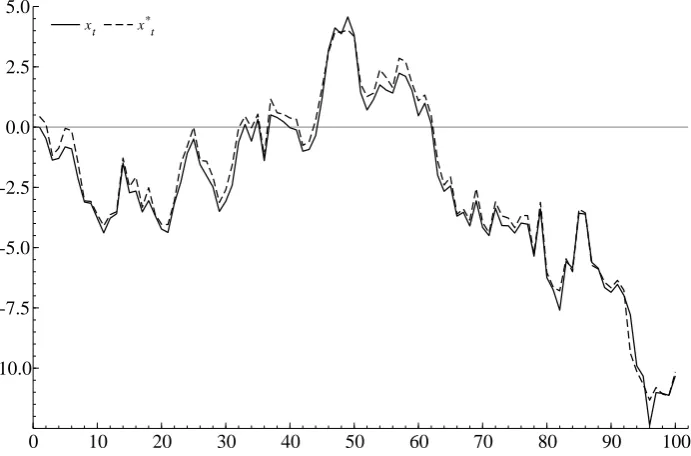
In Figure 5, we report a bootstrap sample path based on the new MEBB algorithm.

We use the same setup as in Section 2 with T = 100 and x0 = 0. The original sample

path and the bootstrap one are different and thus the new algorithm does not mimic the

5_{The tails are of the exponential form, which advocates the use of the trimming algorithm. On the}

(15)

Figure 5: MEBB sample path replication.

xt x*t

0 10 20 30 40 50 60 70 80 90 100

-10.0 -7.5 -5.0 -2.5 0.0 2.5 5.0

xt x*t

Note: The figure reports the sample path xt and the replicated path x∗t by the MEBB.

The true data generating process is given as xt=xt−1+εt, with εt∼N(0,1), x0 = 0, and T = 100.

sample data too closely.

In order to provide evidence that our proposed method works, we report in the left

panel of Figure 6 the empirical rejection frequency of thet-statistic to test forρ= 1 using

the same design as in the previous section. The MEBB rejection frequencies coincide

with the nominal values as required. In the right panel of Figure 6, we present the

distribution of the t-statistic based on the simulated series as well as the distribution of

the corresponding bootstrapped t-statistic based on the MEBB . The two distributions

coincides in the same manner as for the original MEB algorithm, see Figure 3.

By comparing Figure 6 with Figure 2, it is evident that our proposed procedure allows

us to restore the correct size. Indeed, a regression similar to that in (7) gives

τ_i∗ = −0.4541

(0.0354)

− 0.005663

(0.0323)

τi i= 1, . . . ,1000

, (13)

with the adjusted R2 _{= 0}_._{00097. As a further evidence that the MEBB works properly,}

we report in Figure 7 the counterpart of Figure 4. As expected, the absence of correlation

(16)

Figure 6: The MEBB.

(a) Empirical rejection frequencies.

45 Line MEBB

0.0 0.1 0.2 0.3 0.4 0.5 0.6 0.7 0.8 0.9 1.0

0.1 0.2 0.3 0.4 0.5 0.6 0.7 0.8 0.9 1.0

45 Line MEBB

(b) Distribution of the bootstrapped statistic under H0: ρ= 1.

τ τ*

-4 -3 -2 -1 0 1 2 3 4

0.05 0.10 0.15 0.20 0.25 0.30 0.35 0.40

τ τ*

Note: The left panel reports the plot of the empirical rejection frequencies against the nominal levels of the test under H0 : ρ = 1 against HA : |ρ| < 1 with the distribution

approximated by the MEBB. The right panel depicts the distribution of the original t -statistic and the distribution of thet-statistic obtained by bootstrapping underH0 : ρ= 1.

Figure 7: Joint Kernel Density

(a) Gaussian Kernel pdf (b) Contour

-3 -2 -1 0 1 2

(17)

The link between the data generating process and the MEBB draws are weak in this

case and therefore our method is able to preserve the perfect rank correlation locally for

each block and it provides a truly viable and working entropy-based bootstrap algorithm.

4. Simulation Study of the MEBB

In this section, we carry out a comprehensive Monte Carlo simulation study to evaluate

the finite sample properties of the MEBB. We compare the entropy-based resampling

schemes with standard bootstrap approaches, i.e. residual-based bootstrap and

non-parametric block-bootstrapping techniques. The comparison is based on the bootstrapped

empirical rejection frequencies of the t-statistics for testing that the value of the AR(1)

coefficient, ρ, estimated by OLS, equals unity (Dickey-Fuller test). The unit-root set-up

is of particular interest as bootstrapping directly a non-stationary series is not common

practice in the econometric literature. In particular, for non-stationary time series there

exists in the literature only the Continuous Path Block Bootstrap (CPBB) developed by

Paparoditis and Politis (2001) and studied also by Phillips (2010).

Bootstrapping unit-root tests is thus one of the potentially most interesting application

of the entropy-based bootstrap method constituting an alternative to standard

residual-based bootstrapped unit-root tests (see Palm et al. 2007 for a review) which are not easy

to apply when the dependence structure of the residuals is difficult to ascertain.

4.1. Monte Carlo Design

We consider approximating by bootstrapping thet-statistic distribution for the AR(1)

coefficient. As benchmark, we consider the empirical rejection frequencies based on the

standard residuals-based bootstrap (RB) and CPBB. Then, we compute empirical

rejec-tion frequencies for the MEBB.

In particular, we generate a time series according to the following data generating

process

xm,t =ρ0xm,t−1+ηm,t

(18)

where m = 1, . . . , M denotes a realizations of the sample path. Further, we consider

different sample sizes T = {50,100,300} and we set ρ0 = 1 in order to assess the

size, while we consider progressive deviations from the unit root hypothesis, specifically

ρ0 ={0.99 ,0.95,0.90,0.80,0.70,0.60, 0.5}, in order to assess the power.

Moreover, we generate the{ηm,t} series allowing for “progressive” fat-tails by

consid-ering in turn the following distributions

ηt

iid

∼        

      

N(0,1)

T(5)

T(3) ,

with T(k) denoting the standard t-distribution with k degrees of freedom. Next, we fit

an AR(1) model and compute the t-statistic

τm =

ˆ

ρm−1

ˆ

σηm(

PT

t=1x2m,t−1)−1/2

, for testing    

  

H0 : ρ= 1

H1 : |ρ|<1

(14)

where ˆρm=

PT

t=1x2m,t−1

−1

PT

t=1xm,t−1xm,t

is the least squares estimator of the

autore-gressive coefficient and ˆσηm = (T−1)

−1/2₍PT

t=1ηˆm,t2 )1/2 is the residuals standard deviation.

To compute the empirical rejection frequencies, we draw b = 1, . . . , B bootstrapped

samples under H0 denoted{x∗b,m,t}Tt=1 either by resampling from the residuals when using

the RB approach or by resampling directly from levels {xm,t} when using both MEBB

and CPBB.

4.1.1. Residuals Bootstrap

x∗_b,m,₀ =xm,0

x∗_b,m,t =ρ0x∗b,m,t−1 +η

∗

b,m,t t = 1, . . . , T

where η_b,m,t∗ are drawn from the centred residuals nηˆm,t− _T1 PTt=1ηˆm,t

oT

t=1 obtained from the residuals of the regression of xb,m,t on its first lag either parametrically or

(19)

4.1.2. Continuous Path Block Bootstrap

Following Paparoditis and Politis (2001), we implement the CPBB procedure as

fol-lows:

1. We compute the centred residuals

ˆ

um,t =xm,t−xm,t−1−

1

T −1

T

X

t=1

(xm,t−xm,t−1)

and define

˜

xm,t =

   

  

xm,1 t = 1

xm,1+Ptj=2uˆm,j t = 2, . . . , T.

The null is imposed by building the intermediate time-series{˜xm,t}generated through

{ˆum,t}.

2. We choose the block length ` < T and let i0, i1, . . . , iu−1 i.i.d. uniform random

numbers on the set [1,2, . . . , T −`], where u=bT /`c (number of blocks).

3. We build the bootstrapped series of length l =u·` as

x∗_b,m,j =xm,1+ [˜xi0+j−1 −x˜i0] first block

x∗_b,m,rs₊_j =x∗_b,m,r`+ [˜xim+j−x˜ir] (r+ 1)

th _block

for j = 1, . . . , `and r = 1, . . . , u−1.

4.2. Simulation Results

We then use{x∗_b,m,t}T

t=1 to compute the bootstrapped counterpart of (14),

τ_m,b∗ = ρˆ

∗ m,b−1

ˆ

σ∗

ηm,b(

PT

t=1x∗m,b,t−12)−1/2

b = 1, . . . , B (15)

and we select the α-quantile τ_m∗(α) of the distribution of the bootstrapped statistic (at

the mth _{iteration) such that} _B−1PB

b=1I(τ

∗

m,b ≤ τ

∗

m(α)) ≈ α. The empirical rejection

frequencies are computed as

1 M

M

X

m=1

I(τm ≤τm∗(α)), (16)

being a one-sided test with rejection to the left.

To compare the size of the different approaches, we compute (16) forα ∈[0.01 , 0.025,

(20)

works well, as we are simulating under H0, we should observe a graph close to the 450

line.

Figure 8 reports the rejection frequencies under H0 (size) for the bootstrap methods

introduced in the previous paragraphs. For the CPBB and MEBB, the block length is set

to u=bT1/3_{c. Overall, the figures suggest that even for small samples with} _T _{= 50, our}

proposed MEBB provides rejection frequencies close to the nominal level, outperforming

the original MEB.

Figure 9 reports the power curves for the alternative bootstrap procedures. The closest

method to the MEBB is the CPBB, which shows also very similar power to our proposed

method. In conclusion, the MEBB provides a valid alternative to the (unique) existing

bootstrap method, which allows to replicate the levels for non-stationary time series.

In the next section, we extend the MEBB and introduce the Maximum non-extensive

Entropy Block Bootstrap, which is based on the generalization of the non-extensive

en-tropy.

5. Beyond the Shannon Entropy: The Maximum non-extensive Entropy Block Bootstrap

We extend the Maximum Entropy Block Bootstrap to the case when the underlying

principle is driven by maximization of the non-extensive entropy and define the Maximum

non-extensive Entropy Block Bootstrap (MnEBB).6

The key concept of our framework is the generalized Tsallis (1988) entropy defined in

the discrete form as

Hq=−

1

1−q 1−

N

X

i=1 (pi)

q

! ,

and in the continuous form as

6_{The MEBB presented in Section 3 is based on the Shannon entropy. Such an entropy is suitable for}

(21)

Figure 8: Emp irical reje ction freque ncies. (a) T = 50 N (0 , 1)

45 Line PRB ME (Vinod) MEBB Asym NPRB CPBB

0 0.1 0.2 0.3 0.4 0.5 0.6 0.7 0.8 0.9 1 0.1 0.2 0.3 0.4 0.5 0.6 0.7 0.8 0.9 1.0

(b) T = 100 N (0 , 1)

0 0.1 0.2 0.3 0.4 0.5 0.6 0.7 0.8 0.9 1 0.1 0.2 0.3 0.4 0.5 0.6 0.7 0.8 0.9 1.0

(c) T = 300 N (0 , 1)

0 0.1 0.2 0.3 0.4 0.5 0.6 0.7 0.8 0.9 1 0.1 0.2 0.3 0.4 0.5 0.6 0.7 0.8 0.9 1.0

(d) T = 50 T (3)

0 0.1 0.2 0.3 0.4 0.5 0.6 0.7 0.8 0.9 1 0.1 0.2 0.3 0.4 0.5 0.6 0.7 0.8 0.9 1.0

(e) T = 100 T (3)

0 0.1 0.2 0.3 0.4 0.5 0.6 0.7 0.8 0.9 1 0.1 0.2 0.3 0.4 0.5 0.6 0.7 0.8 0.9 1.0

(f ) T = 300 T (3)

45 Line RPB ME (Vinod) MEBB Asym NPRB CPBB

0 0.1 0.2 0.3 0.4 0.5 0.6 0.7 0.8 0.9 1 0.1 0.2 0.3 0.4 0.5 0.6 0.7 0.8 0.9 1.0

(g) T = 50 T (5)

0 0.1 0.2 0.3 0.4 0.5 0.6 0.7 0.8 0.9 1 0.1 0.2 0.3 0.4 0.5 0.6 0.7 0.8 0.9 1.0

(h) T = 100 T (5)

0 0.1 0.2 0.3 0.4 0.5 0.6 0.7 0.8 0.9 1 0.1 0.2 0.3 0.4 0.5 0.6 0.7 0.8 0.9 1.0

(i) T = 300 T (5)

0 0.1 0.2 0.3 0.4 0.5 0.6 0.7 0.8 0.9 1 0.1 0.2 0.3 0.4 0.5 0.6 0.7 0.8 0.9 1.0

Note: The figure rep orts the empirical rejection frequencies for sev eral b o otstrap metho ds. The data generating pro cess is giv en as xt =

xt−

(22)

Figure 9: P o w er of the tests. (a) T = 50 N (0 , 1)

Asym NPRB CPBB PRB ME (Vinod) MEBB

0.5 0.55 0.6 0.65 0.7 0.75 0.8 0.85 0.9 0.95 0.1 0.2 0.3 0.4 0.5 0.6 0.7 0.8 0.9 1.0

(b) T = 100 N (0 , 1)

0.5 0.55 0.6 0.65 0.7 0.75 0.8 0.85 0.9 0.95 0.1 0.2 0.3 0.4 0.5 0.6 0.7 0.8 0.9 1.0

(c) T = 300 N (0 , 1)

0.5 0.55 0.6 0.65 0.7 0.75 0.8 0.85 0.9 0.95 0.1 0.2 0.3 0.4 0.5 0.6 0.7 0.8 0.9 1.0

(d) T = 50 T (3)

0.5 0.55 0.6 0.65 0.7 0.75 0.8 0.85 0.9 0.95 0.1 0.2 0.3 0.4 0.5 0.6 0.7 0.8 0.9 1.0

(e) T = 100 T (3)

0.5 0.55 0.6 0.65 0.7 0.75 0.8 0.85 0.9 0.95 0.1 0.2 0.3 0.4 0.5 0.6 0.7 0.8 0.9 1.0

(f ) T = 300 T (3)

0.5 0.55 0.6 0.65 0.7 0.75 0.8 0.85 0.9 0.95 0.1 0.2 0.3 0.4 0.5 0.6 0.7 0.8 0.9 1.0

(g) T = 50 T (5)

0.5 0.55 0.6 0.65 0.7 0.75 0.8 0.85 0.9 0.95 0.1 0.2 0.3 0.4 0.5 0.6 0.7 0.8 0.9 1.0

(h) T = 100 T (5)

0.5 0.55 0.6 0.65 0.7 0.75 0.8 0.85 0.9 0.95 0.1 0.2 0.3 0.4 0.5 0.6 0.7 0.8 0.9 1.0

(i) T = 300 T (5)

0.5 0.55 0.6 0.65 0.7 0.75 0.8 0.85 0.9 0.95 0.1 0.2 0.3 0.4 0.5 0.6 0.7 0.8 0.9 1.0

The figure depicts the p o w er of the test for sev eral b o otstrap metho ds. The data generating pro cess is giv en as xt =

xt−

(23)

Hq=−

1

1−q 1−

ˆ

dx(p(x))q

! ,

where the parameter q governs the non-extensiveness of the system. The Tsallis entropy

converges to the Shannon entropy in the limit when q →1.

For a given q, the density function fq is given as

fq(x) =

[1−β(1−q)x]1/(1−q)

Zq

, (17)

with normalization constant

Zq =

ˆ

dx[1−β(1−q)x]1/(1−q) .

The non-extensiveness of the system can be expressed for two systemsA and B as

Hq(A+B) = Hq(A) +Hq(B) + (1−q)Hq(A)Hq(B) .

The density function resulting from the optimization of the Tsallis entropy has a finite

integral over the semi-definite interval forq∈(1,2). The limit of this distribution function

is exponential function for q → 1. For q ∈ (1,2), we get power law behaviour and thus

fatter tails for the distribution. For q < 1, we get a non-standard behaviour of the

distribution function as it is infinite over the semi-definite interval and thus it requires

a normalization by an infinite normalization factor. This still allows for a comparison

between the two draws as ∞/∞ ∼ c, but it provides unnecessary complications. As

q → 0, we get uniform distribution, or, fq→0(x) = c/∞, where c does not depend on x.

For q >5/3, we get a distribution with non-existing second moment, or E[x2] =∞.7 _At

q = 2, the first moment cease to exist. In this paper, we explicitly consider q ∈ [1,5/3),

which covers a broad range specifications ranging from the standard Shannon entropy to

cases with non-existent second moments and fat tails.

7_{In general, it would be more appropriate to deal with the} _q_{-expectations, which remain finite and}

(24)

5.1. The MnEBB Algorithm

The MnEBB algorithm is defined as follows. First, the mass preserving constraint

states that, on average, 1/T of the mass of the density function lies in each of the intervals

It. This is achieved by bootstrapping the set xt as a T draws, each from the different

interval It. Second, the mean preserving constraint says that

T

X

t=1

xt=

T

X

t=1

x(t) =

T

X

t=1

mt,

where mt is the mean off(x) over the interval It.

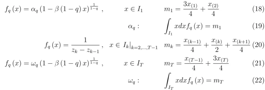
The new framework thus leads to the following choice of the density functions

fq(x) =αq(1−β(1−q)x)

1

1−q _, _x∈_I1 _m1 = 3x(1)

4 +

x(2)

4 (18)

αq:

ˆ

I1

xdxfq(x) =m1 (19)

fq(x) =

1

zk−zk−1

, x∈ Ik|_k₌₂_,...,T−1 mk =

x(k−1)

4 +

x(k)

2 +

x(k+1)

4 (20)

fq(x) =ωq(1−β(1−q)x)

1

1−q , x∈I

T mT =

x(T−1)

4 +

3x(T)

4 (21)

ωq :

ˆ

IT

xdxfq(x) = mT (22)

The remaining structure of the MnEBB algorithm is just as defined for the MEBB.

The choice of q >1 suggests using the distribution with fatter tails than implied by the

standard entropy.

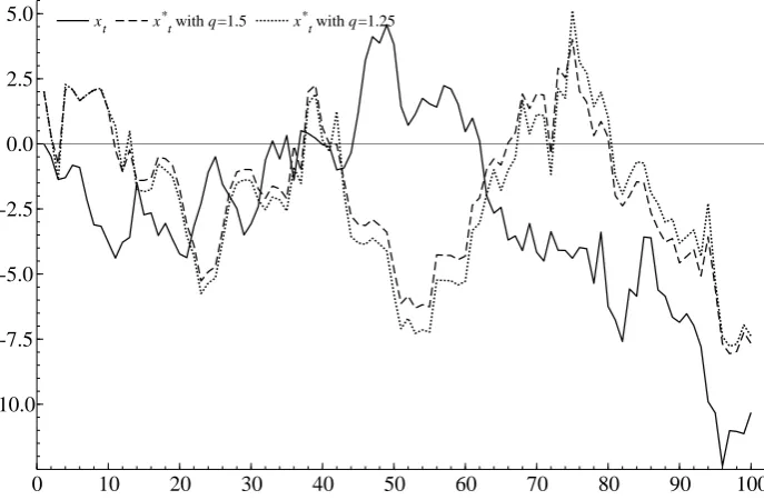
Figure 10 reports a bootstrap sample path based on the new MnEBB algorithm. We

use the same setup as in the previous section with T = 100, y0 = 0 and two values of

non-extensiveness parameter: q = 1.25 and q = 1.5. The figure supports the intuition

that more the non-extensive the system is, the more variation in the replication sample

is present.

5.2. Simulation Results

We replicate the extensive simulation analysis as in Section 4 and focus on the

[image:24.595.86.525.325.475.2]

(25)

Figure 10: MnEBB sample path replication.

xt x*t with q=1.5 x*t with q=1.25

0 10 20 30 40 50 60 70 80 90 100

-10.0 -7.5 -5.0 -2.5 0.0 2.5

5.0 _x_t _x_*t_{with q=1.5} _x_*t_{with q=1.25}

Note: The figure reports the sample path xt and the replicated path x∗t by the MnEBB.

The short-dash line corresponds to MnEBB with q = 1.25 and dot line corresponds to MnEBB with q = 1.5. The true data generating process is given as xt =xt−1 +εt, with

εt∼N(0,1), x0 = 0, and T = 100.

Figure 11 reports the rejection frequencies for three MnEBB methods withq= 1, 1.25,

and 1.5, respectively, introduced in the previous paragraphs. The data generating process

is given as xt = xt−1 +εt, with εt ∼N(0,1), T (3) and T (5), respectively, with x0 = 0,

and T = 100. Overall, the figures suggest that for q = 1.25, the MnEBB underperforms

in terms of size the MEBB. However, with increasing q, the MEBB and MnEBB are

becoming indistinguishable.

Figure 12 reports the power of the alternative bootstrap procedures. The power

sup-ports the inferiority of MnEBB with q = 1.25 to the original MEBB, while the MnEBB

with q = 1.5 is dominating in terms of the power. Therefore, the MnEBB method with

fatter tails provides a significant improvement to the entropy based algorithm even for

the data generating process based on the Gaussian distribution.

6. Conclusions

In this paper, we proposed the Maximum Entropy Block Bootstrap, a fully

[image:25.595.119.463.108.333.2]

(26)

Figure 11: Non-exte nsiv e size. (a) N (0 , 1) q = 1 . 25

45 Line MNEBB

References

Buhlmann, P. (1997). Sieve Bootstrap for Time Series. Bernoulli 3, 123–148.
Davidson, R. and A. Monticini (2014). Heteroskedasticity-and-autocorrelation-consistent
bootstrapping. Technical report, Universit`a Cattolica del Sacro Cuore, Dipartimenti e
Istituti di Scienze Economiche (DISCE).
Efron, B. (1979). Bootstrap Methods: Another Look at the Jackknife. Annals of
Statis-tics 7, 1–26.
K¨unsch, H. (1989). The Jack-knife and the Bootstrap for General Stationary Observations.
Annals of Statistics 17, 1217–1241.
Mammen, E. (1993). Bootstrap and Wild Bootstrap for High Dimensional Linear Models.
Annals of Statistics 21, 255–285.
Palm, F. C., S. Smeekes, and J.-P. Urbain (2007). Bootstrap Unit-Root Tests:
Compar-isons and Extensions. Journal of Time Series Analysis 29, 371–401.
Paparoditis, E. and D. Politis (2001). The Continuous Path Block-Bootstrap. In M. Puri
(Ed.), Asymptotics in Statistics and Probability, pp. 305–320. VSP Publications.
Phillips, P. C. B. (2010). BootstrappingI(1) Data.Journal of Econometrics 158, 280–284.
Politis, D., J. Romano, and M. Wolf (1999). Subsampling. Springer Series in Statistics.
Springer New York.
Tsallis, C. (1988). Possible Generalization of Boltzmann-Gibbs Statistics. Journal of
Statistical Physics 52(1-2), 479–487.
Vinod, H. D. and J. L´opez-de Lacalle (2009). Maximum Entropy Bootstrap for Time
Series: the meboot R Package. Journal of Statistical Software 29, 1–19.
Wu, C.-F. J. (1986). Jackknife, Bootstrap and Other Resampling Methods in Regression