Determination of image quality for added noise as a function of spatial frequency

(1)

Rochester Institute of Technology

RIT Scholar Works

Theses

Thesis/Dissertation Collections

7-1-1989

Determination of image quality for added noise as a

function of spatial frequency

Yun-Ching Kuo

Follow this and additional works at:

http://scholarworks.rit.edu/theses

This Thesis is brought to you for free and open access by the Thesis/Dissertation Collections at RIT Scholar Works. It has been accepted for inclusion

in Theses by an authorized administrator of RIT Scholar Works. For more information, please contact

[email protected]

.

Recommended Citation

(2)

DETERMINATION OF IMAGE OUALITY

FOR ADDED NOISE AS A FUNCTION OF SPATIAL FREOUENCY

by

Yun-Ching Kuo

A.A.

World College of Journalism

(1981)

A thesis submitted in partial fulfillment of the requirements for

the degree of Master of Science in the Center for Imaging science

of Rochester Institute of Technology

July 1989

Signature of the Author

Oenter for Imaging Science

Accepted by

Name Illegible

(3)

Center for imaging Science

Rochester Institute of Technology

Rochester,

New York

CERTIFICATE OF APPROVAL

M.S. DEGREE THESIS

The M.S. Degree Thesis of Yun-Ching Kuo has been examined and

approved by the thesis Committee as satisfactory for the

thesis requirement for the Master of Science degree.

Dr. E.M.

Granger,

Thesis Advisor

Dr. R.L.Easton

Dr. D. Marsh

(4)

THESIS RELEASE PERMISSION FORM

CENTER FOR IMAGING SCIENCE

ROCHESTER INSTITUTE OF TECHNOLOGY

Title of Thesis

: Determination of Image Quality for Added Noise

as a Function of Spatial Frequency

I,

Yun-Ching

Kuo,

hereby

grant

permission

to

the

Wallace Memorial Library of Rochester Institute of Technology to

produce my thesis in whole or in part. Any reproduction will not

be of commerical use or for profit.

Signature

Date

(5)

Determination

of

Image

Quality

for

Added

Noise

as a

Function

of

Spatial

Frequency

by

Yun-Ching

Kuo

Submitted

to

the

Center

for

Imaging

Science

in

partial

fulfillment

of

the

requirements

for

the

Master

of

Science

Degree

at

the

Rochester

Institute

of

Technology

ABSTRACT

The

noise

in

color

images

which

is

referred

to

as

chromatic

noise represents a

distribution

within

three

spectral

bands

and

contributes

to

chromatic

and

achromatic

visual

effects.

The

chromatic

noise

depends

very

strongly

on

the

spatial

frequency

response of

the

visual

system.

Therefore,

this

study

characterizes

the

variation

in

perceived

chromatic

noise

level

and

generates

the

noise

field

to

add

to

the

color

image

samples.

From

these

degraded

images,

we

found

that

noise

in

low

spatial

frequencies

is

much more

disturbing

than

in

the

medium

and

high

spatial

frequency

regions.

The

perceived

quality

scales

of

the

modulated

chromatic

noise

images

were

compared

to

the

subjective

quality

factor

(S.Q.F.)

scales.

By

using

category

analysis,

this

quality

scale

yields

the

S.Q.F.

rating,

and

determines

the

dependence

of

the

spatial

frequency

content

of

chromatic

noise

(6)

TABLE

OF

CONTENTS

I

INTRODUCTION

1

II

BACKGROUND

STUDIES

3

1.

Literature

Review

3

A.

The

MacAdam-Friele

Study

3

B.

Implication

of

the

MacAdam

Data

4

C.

MTF

of

Achromaticity

and

chromaticity

5

2.

Visual

System

8

3.

Image

Quality

and

S.Q.F.

12

4.

Psychophysical

Evaluation

Method

18

5.

Colored

Noise

22

A.

Image

Signal

22

B.

Random

Noise

22

III

OBJECTIVE

25

IV

EXPERIMENTAL

28

1.

Image

Scanning

28

A.

Scanning

Process

28

B.

Image

Size

and

Sampling

33

2.

Random

Noise

Generation

35

3.

Gaussian

Bandpass

Filter

36

4.

Noise

Scaling

40

V

DESIGN

AND

ANALYSIS

61

1.

The

TABLES

TABLE

4

.

1

TABLE

5.1

TABLE

5.2

TABLE

5.3

TABLE

5.4

TABLE

5.5

TABLE

5.6

TABLE

5.7

TABLE

5.8

TABLE

5

.

9

TABLE

5.10

TABLE

6.1

Mean

and

Variance

of

the

Passband

Noise

53

Analysis

of

Variance

for

Rating

Data

67

Comparison

on

the

Rating

Data

68

Observed

Frequencies

72

Observed

Cumulative

Frequencies

73

Observed

Cumulative

Proportions

74

Normal

Deviates

75

Boundary

Mean

Values

Vs.

SQF

Values

78

Regression

Analysis

on

Girl

Imagery

80

Regression

Analysis

on

Mask

Imagery

81

Regression

Analysis

on

Two

Images

82

Analysis

Results

83

(9)

LIST

OF

FIGURES

FIGURE

2.1

FIGURE

2.2

FIGURE

2.3

FIGURE

2.4

FIGURE

2.5

FIGURE

2.6

FIGURE

3.1

FIGURE

3.2

FIGURE

Figure

FIGURE

4.1

4.2

4.3

4.4

4.5

4.6

7

8

.9 .10 .11 ,12 ,13 ,14 .15 ,16 ,17 ,18 ,19

4.20

MTF

of

Visual

Achromaticity

and

Chromaticity

7

MTF

of

Human

Observer

8

Predicted Versus

Observed

Brightness

Distribution

9

Spectral

Luminous

Efficiency

for

Normal

Observers

11

Subjective

Quality

Factor

Passband

16

Magnification

Comparison

17

Noise

Distribution

on

Visual

Transfer

Function

26

Noise

Distribution

vs.

Subjective

Quality

Scales

26

Girl

Image

28

Mask

Image

29

Comparison

of

Two

Images

-I

30

Comparison

of

Two

Images

-II

31

Imaging Scanning

and

Process

Sequence

32

Low

Frequency

Gaussian

Filter

37

Medium

Frequency

Gaussian

Filter

38

High

Frequency

Gaussian

Filter

39

Noise

Scaling

Process

42

Low

Frequency

Noise

44

Medium

Frequency

Noise

45

High

Frequency

Noise

46

Comparison

of

Girl

Images

-

I

47

Comparison

of

Girl

Images

-II

48

Comparison

of

Girl

Images

-III

49

Comparison

of

Mask

Images

-IV

50

Comparison

of

Mask

Images

-V

51

Comparison

of

Mask

Images

-VI

52

(10)

FIGURE

4.21

FIGURE

4.22

FIGURE

4.23

FIGURE

4.2 4

FIGURE

5.1

FIGURE

6.1

FIGURE

6.2

FIGURE

6.3

FIGURE

6.4

High

Frequency

Noise

Girl

Image

57

Low

Frequency

Noise

Mask

Image

58

Medium

Frequency

Noise

Mask

Image

5 9

High

Frequency

Noise

Mask

Image

60

Average

Rating

vs.

Noise

Levels

69

Spatial

Frequency

Response

vs .

SQF

-I

85

Spatial

Frequency

Response

vs.

SQF

-

II

85

Noise

Distribution

on

Visual

Transfer

Function

86

Comparison

of

Hypothesis

and

Experiment

result

(11)

I.

INTRODUCTION

The

questions

of

how

to

characterize

image

quality

and

what

constitute

optimum

visual

quality

are common

to

many

applications.

This

study

is

concerned

with

characterizing

perceived

quality

of

images

with noise and

developing

a

technology-independent

method

for

predicting

image

quality.

The

principal

source

of

noise

will

be

regarded as

the

random

noise

of

the

system.

In

the

study

of color

image

quality,

the

most

important

factor

is

the

luminance

effect.

The

noise of color

images

is

a

distribution

in

three

spectral

bands:

red,

green,

and

blue.

By

varying

the

noise

level,

the

effective noise

in

these

frequency

regions will contribute

to

chromatic

and

achromatic

visual

effects.

The

report

investigates

the

image

quality

for

added

noise

as

a

function

of spatial

frequency.

This

study

will show

that

the

visual effect of

the

noise

exhibits

a

very

powerful

dependence

on

the

spatial

frequency.

If

one

is

to

relate subjective and

objective

quality

in

absolute

terms,

it

is

necessary

to

account

for

the

various

functional

properties

of

the

human

visual system.

The

visual

system

is

known

to

be

complex

in

its

behavior,

for

example,

it

often

appears

to

have

non-linear response

to

complex

stimulus

patterns,

(e.g.

the

(12)

various

brightness

illusions1

and

the

receptive

field

characteristics2).

Thus

a visual model

for

image

quality

perception

must

accomodate

a

linear

objective

relationship

with a

nonlinear

subjective

relationship.

An

image

quality

merit

function

(Subjective

Quality

Factor)

has

been

proposed as an objective

figure

of merit which

can

be

easily

calculated and

directly

measured

in

practice and

which will correlate with subjective rank3.

The

results

have

shown

that

the

image

quality

merit

function

is

able

to

predict

image

guality

within normal reader

error and

is

linearly

correlated with

the

measured

data.

In

this

study,

we used

the

SQF

to

define

the

quality

of

the

images

and

demonstrated

a correlation of

96%

with

the

measured

data.

The

visual

efficiency

for

noise perception exhibits a

linear

objective

relationship

in

this

study.

The

variation of

the

perceived color

image

in

different

noise

levels

were correlated

with

the

subject's perception of

image

guality.

(13)

II.

BACKGROUND

STUDIES

1

.

LITERATURE

REVIEW

A.

The

MacAdam-Friele

Study

-In

1942,

MacAdam

published

results of

experiments

in

which a single observer

made

25,000

observations

of color

differences

from

25

selected

points

in

the

x-y

chromaticity

diagram4.

These

experiments were carried

out

by having

observers view a pair of visual

fields

to

determine

the

point at which one

field

became

visually

different

from

the

other.

The

experiment5

was

designed

to

"measure"

the

distance

shift

in

each

direction

in

the

x-y

diagram

that

would produce a

just-noticeable,

or

threshold,

color

difference.

Because

of

the

dependence

of such experiments on

the

level

of

illumination

and

adaptation of

the

eye,

MacAdam

surrounded

the

test

fields

with a

neutral

gray

field

to

stimulate

the

object mode without

dis

tracting

from

the

visual

task.

The

results of

his

experiments show

that

the

eye can

discriminate

between

small changes

in

x-y

coordinates

in

the

violet

region,

while

the

eye

is

least

sensitive

to

chromaticity

changes

in

the

green region of

the

diagram.

Friele

(1961)6 used

the

Muller

(1930)7

theory

of color

(14)

seeking.

He

used

MacAdam

's

data

on

equally

perceptible

intervals

to

guide

the

selection

of

tristimulus

response

functions.

Friele

followed

the

Muller

theory

in

proposing

that

the

lightness-response

function

L

is

the

sum of red-receptor and green-receptor

signals

(R+G)

.

The

redness-greenness

_response

function

A

results

is

the

difference

between

the

same

two

signals

(R-G)

.

The

yellowness-blueness

response

function

B

is

the

difference

between

the

blue-receptor

signal and

the

red-plus-green average :

R+G

Z

B

]

.

B

.

Implication

of

the

MacAdam

Data

-The

threshold

ellipsoids

of

MacAdam

are

transformed

to

a coordinate system of

fundamental

primaries.

The

thresholds

of color

discrimination

can ft

be

described

as a Weber-Fechnerian

differential

sensitivity

in

the

fundamental

process,

i.e.

equal stimulus ratios are predicted

to

elicit equal

sensory

differences.

This

is

combined with one

summation process

(lightness)

and

two

chromatic

processes

(red-green,

yellow-blue)

.

When

a small signal

is

combined with a

large

signal,

the

threshold

of

the

small signal

is

enhanced

to

overcome

the

"noise"

of

the

larger.

If

a small signal

from

one receptor

is

combined

with a

large

signal

from

another

receptor,

the

effective

threshold

for

the

first

receptor

is

limited

by

the

"noise" of

the

second.

The

brightness

of

the

surrounding

field

also

limits

the

thresholds

.

(15)

-4-The

problems

of visual adaption of

the

eye and

the

spatial

frequency

suggested

a

further

study

which varys

the

brightness

(amplitude

of

the

noise)

of

the

subject

to

produce a new color

perception

formed

by

the

three

spectral

bands.

Also,

the

variations of

the

noise

amplitude

can

be

the

human

color vision

perception.

Therefore,

the

relationship

of spatial

frequency

and

image

quality

will also

be

examined

in

this

study.

C.

MTF

of

Achromaticity

and

Chromaticity

-Many

studies

in

the

field

of

image

quality

definition

have

noticed

that

a

perceptible

difference

in

image

quality

can

be

obtained

by

changing

the

scale of either

the

point spread

function

or

the

modulation

transfer.

This

tells

us

that

image

quality

is

logarithmic

spatial

frequency

weighting

of

the

system optical

transfer

function

(OTF)

.

Specifically,

image

quality

correlates

with

the

area under

the

system

OTF

when

displayed

on a

log

spatial

frequency

scale.

The

quality

of a visual

image

is

the

scale

of

the

image

on

the

retina.

The

human

visual system

has

a

modulation

transfer

function

(MTF)

with

broad

peak response at

6

cycles

per

degree

(cpd)

.

The

eye response can

be

correlated

with

quality

rank

and

computed rank

if

the

"true"

eye

MTF

is

used

in

the

calculation of

quality

rank.

In

fact,

computations

that

use

only

the

one-dimensional

MTF

have

proven quite

successful

in

predicting

quality

rank

for

two-dimensional

image

structure.

(16)

includes

the

proper

weighting

function

to

describe

the

two-dimensional

visual

properties

of

the

image.

The

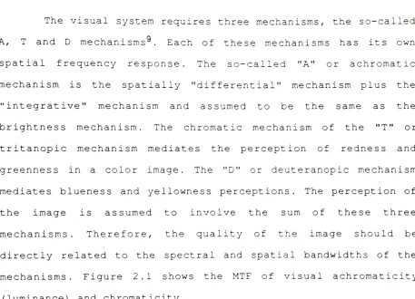
visual system

requires

three

mechanisms,

the

so-called

A,

T

and

D

mechanisms9.

Each

of

these

mechanisms

has

its

own

spatial

frequency

response.

The

so-called "A" or achromatic

mechanism

is

the

spatially

"differential"

mechanism plus

the

"integrative"

mechanism and assumed

to

be

the

same as

the

brightness

mechanism.

The

chromatic mechanism of

the

"T" or

tritanopic

mechanism mediates

the

perception of redness and

greenness

in

a color

image.

The

"D"

or

deuteranopic

mechanism

mediates

blueness

and yellowness perceptions.

The

perception of

the

image

is

assumed

to

involve

the

sum of

these

three

mechanisms.

Therefore,

the

quality

of

the

image

should

be

directly

the

spectral and spatial

bandwidths

of

the

mechanisms.

Figure

2.1

shows

the

MTF

of visual

achromaticity

(luminance)

and chromaticity. [image:16.553.48.505.121.451.2]

(17)

-6-0.3

1.0

3.0

10.0

Spatial

Frequency

-cpd

30.0

[image:17.553.69.387.78.317.2]

(18)

2.

VISUAL

SYSTEM

Studies

of

the

modulation

transfer

characteristics of

the

visual system show

that

the

visual system's response

to

luminous

sine-waves

defines

a visual system modulation

transfer

function

(MTF)10

which

has

a

very

broad

peak with maximum response at

6

cycles per

degree

(cpd)

.

A

typically

observed

MTF

is

shown

in

Figure

2.2

Measurements

down

to

very

low

spatial

frequencies

show

that

the

MTF

continues

to

decrease

in

linear

fashion.

From

the

measurement of

the

visual system's response

to

the

modulus of

the

sine-wave,

a

Image

Quality

Merit

Function

(IQMF)

c can

be

derived

.

0.1

1.0

10.0

100.0

Spatial

Frequency

-

Cycles/Degree

Figure

2.2

MTF

OF

HUMAN

OBSERVER

Studies13

of

the

visual

field

demonstrate

a

linear

organization of

inhibitory

and

excitatory

regions of

the

field.

The

response of

the

elementary

visual

fields

is

turned

to

respond

(19)

-8-to

lines

of a given

orientation

that

traverse

a given

locality

on

the

retina.

The

action of

the

visual

fields

suggests

that

the

visual

information

is

collected

in

one

dimension

by

the

spatial

differencing

mechanism.

Cornsweet

performed

a

Fourier

analysis of a

bar

of

light

and

calculated

its

hypothetical

appearance after

processing

by

the

measured system

MTF.

The

results of

his

analysis are shown

in

Figure

2.3.

Note

the

large

difference

between

the

calculated

appearance

(Figure

2.3b)

and

the

appearance of a

bar

as perceived

by

human

observer

(Figure

2.3c)

.

:*7>

(a)

j|

timul

=

5

*

S

J3

(b)

cSo

>

r

Computed Response

<u > f>

(c)

t?

.a s O O

Observed

Response

Figure

2.3

PERDICTED

VERSUS

OBSERVED

BRIGHTNESS

DISTRIBUTION

(20)

perception of

the

object

indicates

that

higher-order

processes

in

the

brain

are

performing

something

analogous

to

_an

integration

of

the

differential

spatial

information

derived

from

the

early

visual

processing

stage.

Without

the

"integration"

process,

the

observer would report

the

bar

as calculated

by

Cornsweet

(Figure

2.3b)

.

From

these

studies,

we can assume

that

the

spatial action

of

the

visual system can

be

modeled

in

two

stages;

the

first

is

spatially

differential

and orientation selective.

This

stage

is

followed

by

an

integrative

process which sums

the

contributions

of

the

differential

stages

to

produce

the

visual

field.

The

second stage

is

assumed

to

be

non-directional

in

nature.

This

model of visual system

is

called subjective

quality

factor.

To

model

the

color vision

system,

we need

to

consider

the

spectral response of

the

system.

Color

vision requires at

least

three

mechanisms .

Experience

with color

television

indicates

that

the

luminance

(black-and-white)

component of color vision

is

most

important

in

maintaining

picture

quality

and

that

two

chromatic

components

play

a much smaller role.

In

these

studies of color

image

quality, we

found

that

the

luminance

component was

the

only

significant contributor

to

image

quality

except

for

some cases

with extreme chromatic aberration.

Therefore,

for

a color

image

which

is

good color

balance

only

the

luminance

mechanism

contributes

significantly

to

image

quality

considerations.

The

sp<

2.4

.

10

jectral

luminosity

response15

(21)

1.0,

400

500

600

Wavelength

-nm

700

Figure

2

.

4

SPECTRAL

LUMINOUS

EFFICIENCY

FOR

NORMAL

OBSERVERS

(22)

3.

IMAGE

QUALITY

AND

S.Q.F.

Images

are

produced

for

viewing

by

humans

or

for

inter

pretation

by

computers.

The

viewing

situation

is

either

a

"performance"

or a

"non-performance

"

situation

depending

on

whether an

immediate

active

response

to

the

image

is

expected.

Computer

vision

applications

always

have

the

character of

performance

situations.

Image

in

graphic

arts

technology

are

viewed

for

information

and

pleasure

in

a

non-performance

manner.

Because

image

quality

is

instrumental

in

determining

the

magnitude

of

information

which can

be

extracted

from

an

image

as

well as

image

outlook.

It

important

in

both

types

of

viewing

situtions

.

From

the

standpoint of

research,

image

quality

consitutes

a research

area

of

its

own.

This

is

because

the

problems

of

image

quality

in

different

applications

have

many

common

features.

The

topics

of

study

in

the

area of

quality

can

be

roughly

divided

to

three

categories:

-

image

quality

components and measurement of

quality,

relationships

between

process

physics,

chemistry,

process

parameters or

image

processing

algorithms and

image

quality

and

- _{relationships}

between

human

visual

performance

and

image

quality

.

(23)

Our

prime

interest

in

this

study

is

the

specification of

color

image

quality;

therefore

we will use

the

Subjective

Quality

Factor

(S.Q.F.)

to

define

image

quality.

SQF

was

introduced

by

Granger

and

Cupery17,

and

incorporates

a

weighting

function

to

simulate

the

visual

process

outlined

in

the

last

section.

The

integration

performed

by

the

higher

process

is

simulated

by

weighting

the

visual system

MTF

by

a

1/f

factor

where

f

is

the

spatial

frequency.

Application

of

this

factor

in

the

frequency

domain

is

equivalent

to

performing

an

integration

in

the

spatial

domain.

The

weight

factor

can

be

converted

to

a convenient

form

by

noting,

that;

df

d

(

In

f

)

=

.

Thus,

a

logarithmic

spatial

frequency

weight

function

also

simulates

the

assumed spatial

integration.

The

image

quality

merit

function

can

be

obtained

for

a

two-dimensional

optical

system

OTF

by

describing

the

system

OTF

in

polar

coordinates

and

performing

the

following

integration

to

simulate

the

assumed

action of

the

visual system:

SQF

=

K

J

|

|T

(lnf,6)

I

T

e

(Inf)

!

d9

d(lnf)

,

In

a

0

where

%

(ln

f,

8

)

is

the

system

OTF

expressed

in

polar

coordinates and

log-spatial-frequency

coordinates.

T

(In

f)

is

the

one-dimensional visual system

MTF,

is

the

azimuth

angle,

and

(24)

f

is

the

spatial

frequency

in

_cycles _per

degree.

The

normalizing

constant

K

is

the

inverse

of

the

above equation with

the

system

OTF

set

to

unity.

The

lower

limit

of spatial

frequency

in

the

integration,

a,

is

chosen as

the

limit

of

the

range of

image

quality

to

be

considered.

Since

spatial

frequency

is

expressed

in

cycles per

degree

of visual

angle,

this

form

of

the

integral

takes

into

account

the

scale of

the

image

on

the

retina.

Therefore,

by

definition,

SQF

includes

the

system magnification .

The

eye

response,

T

(f

)

_,

has

c

a

broad

bandpass

structure

in

the

spatial

frequency

domain

as

illustrated

in

Figure

2.2.

This

response can

be

approximated

by

a

retangular spatial

frequency

response

between

the

limits

of

3

cpd and

12

cpd.

This

approximation eliminates

the

one-dimensional

visual system

MTF

and allows

this

simplification:

In 12

2

71

SQF

=

K

J

I

(lnf.9

)

I

d8

d(lnf)

.

In3

0

The

SQF

merit

function

can

be

extended

to

color

images

by

using

a spectral weight which

includes

the

spectral response of

the

visual system and

that

of

the

transparancy

or print material.

Therefore,

the

image

quality

of an optical system

is

given

by:

In 12 2n

700

SQF

=

kJ

J J

I

T(Inf,9,X)

Sxvxdx

I

d6

d(lnf)

In

3

0

400

where

T

(In

f,

8,

X)

is

the

spectral

OTF

in

polar

coordinates,

[image:24.553.56.508.71.400.2]

(25)

14-S

X

is

the

sPectral

transmittance

or

reflectance

of a neutral

(white)

reproduced

in

the

print

or

transparency,

and

V.

is

the

spectral

luminosity

response

of

the

visual system.

The

wavelength

X

is

measured

in

nanometers

and

the

spatial

frequency

f

in

cycles

per

degree

.

One

convenience

offered

by

this

equation

is

that

the

given

value of

SQF

is

easily

evaluated

graphically.

The

eye response

has

a

broad bandpass

structure

in

the

spatial

frequency

domain

as

illustrated

in

Figure

2.2.

This

response can

be

approximated

by

a

rectangular spatial

frequency

response

between

the

limits

of

3

cpd

and

12

cpd.

The

SQF

merit

function

can

be

extended

to

color

images

by

using

a spectral weight which

includes

the

spectral

response of

the

visual system and

that

of

the

transparency

or

print material.

The

given value of

the

SQF

is

easily

evaluated

graphically.

The

quality

rank

is

simply

the

area under

the

MTF

between

the

two

spatial

frequency

limits

as

shown

in

Figure

2.5.

S.Q.F.

was

defined

to

duplicate

the

operation of

the

human

visual system

as

shown

in

Figure

2.5,

which

shows

that

human

are

able

to

utilize

only

a small

band

of spatial

frequencies.

The

position of

the

SQF

passband on

the

linear

spatial

frequency

axis

can

be

readily

located

in

the

following

manner.

A

viewing

distance

of

34

cm will

define

unit magnification.

This

viewing

condition places

the

center of

the

SQF

passband

conveniently

at

a

spatial

frequency

of

1

cycle per mm

at

the

image

plane.

Using

(26)

mm

is

just

equal

to

the

magnification

used

to

view

the

image

PASSBAND

APPROXIMATION

VISUAL SYSTEM

<>

34 CM VIEWING

DISTANCE

3

6

12

Spatial

Frequency

-cycles/mm

Figure

2.5

SUBJECTIVE

QUALITY

FACTOR

PASSBAND

Therefore,

at a normal

viewing

distance

of

34

cm,

this

region of

sharp

visual response corresponds

to

a spatial

frequency

region

of

0.5

to

2.0

lines

per mm.

We

have

found

that

we can

predict

with excellent

accuracy

the

quality

name response of

a

human

observer

to

the

information

available

in

this

spatial

frequency

region.

Figure

2.6

illustrates

another

advantage

of

the

log

frequency

weighting.

Two

separate

S.Q.F.

regions

(Ml

and

M2)

are

shown.

These

represent

the

change

in

visual response

to

a given

image

as

a

function

of magnification.

Greater

magnification

pushes

the

passband

to

higher

spatial

frequencies.

Two

systems

can

also

be

evaluated at

a

variety

of

magnifications

by

converting

the

angular spatial

frequency

coordinates

to

linear

coordinates.

(27)

-16-SQF(A)>SQF(B)

SQF(A)<SQF(B)

1.0

1

<L)

V

lens

A

o*>

c

\

Ni

CO k_ 1 ez o CD

15

~^T"

^-^^

T3

O

lens

B

z

M 1

M2

^

\

1

w

Log

Spatial

Frequency

Figure

2.6

MAGNIFICATION

COMPARISON

(28)

4

.PSYCHOPHYSICAL

EVALUATION

METHOD

In

studies

of

color

reproduction,

it

is

usually

desirable

to

scale

the

"quality"

of

images

to

predict

the

subjective effect

of

variations

in

the

physical

parameters

of

the

reproduction

system.

In

this

study,

observers

are

required

to

indicate

their

relative

preferences

for

the

individual

members of

a

group

of

dissimilar

color

images.

When

the

number of stimuli are

fixed

and

their

characteristics are

invariant,

there

are a number of

tasks

that

observers

may

perform

to

derive

the

data

from

which a

quality

scale

may

be

constructed.

Instructions

for

performing

such

tasks

are :

1)

Rate

each stimulus on

a

scale

of n equal

steps.

2)

Sort

the

stimuli

into

n

piles

or groups so

that

the

intervals

between

the

piles are

subjectively

equal.

3)

Given

that

stimulus

A

has

a value of

R

units,

report

the

value of stimulus

B.

These

tasks

are quantitative

judgement

methods;

that

is,

the

unit of measurement

is

obtained

directly

from

quantitative

judgements

of stimuli with respect

to

the

attribute.

The

task

set

for

the

observer always requires more

than

the

ability

to

differentiate

stimuli on

the

basis

of

their

order.

(29)

There

are

a number of

methods

to

perform

the

multiple

presentation

for

quantitative-judgement

tasks.

The

method used

for

this

study

recognizes

as

successive

categories or categorical

judgment.

The

scheme

requires

an observer

to

make an absolute or

direct

estimate

of

the

magnitude

of

quality

differences

among

stimuli and

to

classify

each

stimulus

in

one of several

category

boundaries

as

if

they

exhibited

the

dispersion

characteristics

associated

with

stimulus

order

in

comparative

judgment.

The

Law

of

Categorical

Judgment19

assumes

that

the

response continuum

may

be

divided

into

a specified number of

ordered categories or steps.

Owing

to

various

factors,

a given

category

boundary

is

not

always

located

at a

particular

point,

but

rather over a range of position

described

by

an

associated

normal

distribution.

The

observer

then

classifies

a

given

stimulus

below

a

given

category

boundary

whenever

the

value

of

the

stimulus

on

the

response continuum

is

less

than

that

of

the

category

boundary.

Essentially,

this

amounts

to

assuming

that

the

boundaries

between

adjacent categories

behave

like

stimuli,

and

it

is

possible

by

alternative

data-reduction

techniques

to

scale

either on

the

basis

of

the

category

limits

or

on

the

central

(30)

Procedures

directly

analogous

to

those

used

in

deriving

the

Law

of

Comparative

judgement

lead

to

a

formal

expression of

the

law

of

categorical

judgement,

tg

-Rj

=

Zjg

(Sj

2

+

sg

2

-2rjg

Sj sg

)

1/2

,

where

g

= _mean

location

of

the

g

th

category

boundary;

sg

=

dispersion

of

the

g

th

category

boundary;

rjg

=

the

correlation

between

position

of

stimulus

j

and

category

boundary

g

;

Zjg

=

the

standard

normal

deviate

corresponding

to

the

proportion

of

times

that

stimulus

j

is

sorted

below

boundary

g.

In

this

study,

we

make

simplifying

assumptions

that

the

covariance

between

stimuli

is

constant

and

that

the

variance

of

the

distribution

of

discriminal

difference

is

constant20.

This

leads

to

a simplified statement:

t

g

R

j

-

Z

jg

K'

where

K

is

a constant.

It

is,

then,

to

derive

an

interval

scale

of subjective

quality

by

this

method.

(31)

The

categorical

judgement

provides

a psychophysical method

for

evaluating

color

images

that

is

most economical of

equipment,

experimental

labor,

and observer skill.

In

other

words,

the

psychophysical method

for

evaluating

the

quality

of color

images

(32)

5.

COLORED

NOISE

A

.

Image

Signal

-A

two-dimensional

chromatic

image

can

be

defined

in

terms

of

the

image

signal

S

which represents

it.

S

is

a

function

of

wavelength

and

spatial coordinates.

This

is

to

say

that

image

signal

can

be

written

as

follows:

image

signal

=

S

[

>,

,

x,

y

]

,

where

X

is

the

spectral

luminance

from

400

to

700

nanometers

and

x

and

y

are spatial

coordinates.

In

a

digital

reproduction

process,

an original

image

(called

input)

undergoes several process steps

before

the

final

print

is

obtained.

These

steps

include

sampling

and

digitiza

tion,

halftoning,

and output

imaging

(printing)

and

modify

the

image

signal

(e.g.

they

add

noise)

.

Apart

from

halftoning,

the

process

steps

can

be

approximately

depicted

as

spatially

linear

operations

.

B

.

Random

Noise

-There

is

always some

level

of

noise

in

an

image

from

scattering

of

the

light,

the

imaging

electronics,

the

formation

of

image

itself.

This

noise

interferes

with

the

color

and

luminance

of

the

image.

The

analysis of noise

in

recorded

images

has

been

extensively

described

in

the

literature.

Particular

interests

(33)

-22-have

included

Fourier

analysis

and

micro-densitometry,

mathe

matical

models

of

image-structure

statistics,

and

the

psycho

physical

attributes

of

image

noise,

i.e.

graininess .

In

this

study,

the

system

noise

will

be

investigated

as a random

variable,

termed

"colored

random noise"

to

describe

an unknown

contaminating

signals.

When

a signal

is

recorded,

an undesired

contaminating

random signal will

be

superimposed

upon

the

desired

signal.

The

functional

form

of

this

noise

is

not

easy

to

express,

even

if

its

origin

is

known.

By

observing

the

noise

for

a period of

time,

we

can

develop

some

knowledge

of

its

characteristics

though

it

can

never

be

predicted

in

detail.

Thus

the

concept of a random

variable

may

be

a useful

tool

in

dealing

with noise .

When

we refer

to

a random

variable,

we mean

that

it

is

an

unknown

function

with a

known

autocorrelation.

Since

the

auto

correlation

function

of

this

random variable can

be

estimated,

so

can

its

power spectrum.

The

phase spectrum cannot

be

determined

Indeed,

the

ensemble

is

composed of

infinitely

many

functions

that

differ

only

in

their

phase spectra.

The

contrast of color

images

may

be

disturbed

in

brightness

or chromaticity.

In

addition,

the

spatial

frequency

character of

the

noise must also

be

investigated.

The

effect

of

colored noise

depends

on

the

response

properties

of

the

human

(34)

may

not

affect

our

ability

to

evaluate

the

performance of

the

image.

In

a medical

imaging

context,

for

example,

there

may

be

high-frequency

"noise".

If

the

object

to

be

detected

has

mainly

low

spatial

frequency

components,

the

"noise"

may

not affect

the

detectability

of

the

"signal".

That

is,

we could

very

well see

the

graininess of an

image

without

having

it

affect our

ability

to

make out

the

signal.

(35)

24-III.

OB.-rEr.TTVR

In

studies

of color

reproduction,

it

is

necessary

to

scale

the

"quality"

of

images

to

predict

the

subjective effect of

variations

in

the

physical

parameters

of

the

reproduction

systems.

The

effect

of

chromatic

noise modulation will

degrade

the

perception on

the

images.

The

object

for

this

experiment

is

to

find

the

effect

of

noise

on

image

quality.

Studies

of

unsharp

masking

indicate

that

the

bandpass

filter

should

be

located

within

the

medium spatial

frequency

band

where

the

visual

response

is

most

sensitive

to

maximize

image

quality.

This

would

suggest

that

noise

is

most

disruptive

at medium

frequencies.

A

diagram

of

the

spatial

frequency

distribution

of

the

noise

vs.

the

luminance

transfer

function

of

human

visual system

is

shown on

Figure

3.1.

Three

narrow

noise

bands

will

be

used

in

this

study

of

image

quality.

The

hypothesis

of

this

study

is

that

there

will

be

a

much greater

sensitivity

to

chromatic

noise

in

the

medium

frequency

region.

The

expected

trend

for

noise perception

in

different

spatial

frequency

regions versus subjective

image

quality

is

(36)

0.1

"Ol

i~0

To"

Spatial

Frequency

-cpd

Figure

3

.

1

NOISE

DISTRIBUTION

ON

VISUAL

TRANSFER

FUNCTION

Low

Medium

High

Spatial

Frequency

Regions

Figure

3.2

NOISE

DISTRIBUTION

VS.

SUBJECTIVE

QUALITY

SCALES

This

figure

suggest

that

noise

in

the

medium

frequency

region

would

be

most

destructive

to

image

quality.

The

different

noise

levels

for

the

image

indicates

the

noise

perception

trend

in

the

three

spatial

frequency

regions.

The

standard

deviation

of

[image:36.553.64.474.60.700.2]

(37)

-26-the

noise

level

will

be

converted

to

digital

count.

We

expect

that

the

reduction

in

image

quality

would

have

a expected

diagram

as shown

in

this

figure

.

The

objective

of

this

study

is

to

add noise

to

an

image

in

three

distinct

narrow spatial

frequency

regions and

to

study

the

loss

of

image

quality

as a

function

of noise

level

and noise

frequency

location.

The

method of

category

scaling

will

be

used

to

scale

the

subjective evaluation of

image

quality.

The

subjective

quality

factor

will

be

used

to

correlate

the

(38)

IV.

EXPERTMT.NT&T.

1

.

IMAGE

SCANNING

A.

Scanning

Process

-Two

continuous-tone color

images

which contain

low,

medium,

and

high

spatial

frequency

information

are used

in

this

study.

The

images

are

denoted

"Girl"

and "Mask"

and

are

shown

in

Figures

4.1

and

4.2.

These

two

images

were

compared

by

analyzing

their

radial power

spectra,

i.e.

the

power

spectrum

integrated

over

2

radians.

Figure

4.1

GIRL

IMAGE

[image:38.553.153.420.371.643.2]

(39)

Figure

4

.

2

MASK

IMAGE

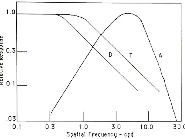
The

radial spatial

frequency

tells

the

image

signals

vary

as

a

function

of spatial

coordinates.

Images

with

slowly

varying

patterns

have

predominantly

low

spatial

frequencies,

and

those

with much

detail

and

sharp

edges

have

high

spatial

frequencies.

Figure

4.3

shows

the

radial power

spectrum

of

these

two

images.

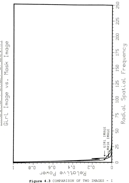
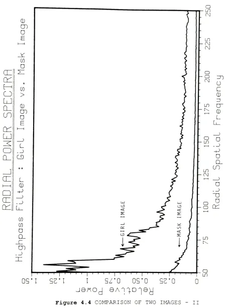
Figure

4.4

shows

the

differences

between

the

Girl

image

and

the

Mask

image

after

highpass

filtering.

It

proves

that

the

Girl

image

has

more

high

frequency

information.

The

Mask

image

(40)

CT

CD

C

o

F

E-<

CJ

i i

ri i

CL_

CO

o

CO

^

(H

LJ

a

CO

^

>

o

n

CD

_j

a

F

en

1 1

CE

L

QZ

CD

CD UJ

s: <c

I

' r

t r

o

-m

.

CM

"

m

-oo

.

CM

a

-a

.

CM

=n

in

u

-1\

L_

- ^

CD

Z5

o~ "

o

CD

-LT)

L

L_

"

LO

n

-CM

t __> +>

a

o

Q_

-a

U )

r 1

a

LO

..j t\

u

D

Lr^

O

LO

CM

a

8'0

9'0

fr'O

Z'O

J8AOJ

9An^D^|9y

Figure

4.3

COMPARISON

OF

TWO

IMAGES

-I

[image:40.553.73.503.58.666.2]

(41)

CD

en

0

F

J

CO

0

en

JZ

(H

E--CO

CJ

>

LjJ

ci_

CO

CD

0

F

ct:

i

LJ

^

(

LJ

-_J>

Q_

CD

_J aa

CE

L

1 i

CD

Q

-H>

CE

-_)

or

Li_

CO

O

D_

._)

HI

~

I T i i i

o

Lfl

CM

0

OS"

I

SZ"I

I

SZ'O

0S"0

Sc"0

Figure

4.4

COMPARISON

OF

TWO

IMAGES

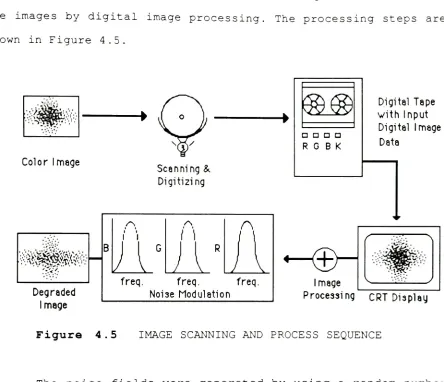
[image:41.553.52.500.60.674.2]

(42)

The

two

images

were

scanned

and

digitized

by

scanner

into

a

magnetic

tape

file.

The

different

noise

samples were added

to

the

images

by

digital

image

processing.

The

processing

steps are

shown

in

Figure

4.5.

Color Image

Digital Tape

with

Input

Digital Image

Data

Scanning

&

Digitizing

Degraded

Image

i i

i

j \

B

11'

){

{

freq.

Noise

Modulation

Processing

CRT

Display

Figure

4

.

5

IMAGE

SCANNING

AND

PROCESS

SEQUENCE

The

noise

fields

were generated

by

using

a random

number

generator

to

create

the

random noise with zero

mean,

uncorrelated

feature,

and unit variance.

This

random

noise

field

can

produce

a

salt-and-pepper effect

particularly

visible

in

flat

(uniformly

gray)

fields.

The

images

were

digitized

by

HELL

Chromagraph

DC-300

scanner

into

a

512

x

512

array

at

8

bits/pixel.

Image

processing

steps

were performed on

the

VAX-8600

computer

system.

[image:42.553.61.505.102.484.2]

(43)

32-Random

noise

was

added

to

the

images,

which were

then

displayed

on and

photographed

off a color

CRT

monitor.

B.

Image

Size

and

Sampling

-The

sampling

theorem

states

that

any

band-limited

function

can

be

specified

exactly

by

its

sampled

values

at regular

intervals,

provided

that

the

intervals

are

smaller

than

specified

by

the

Nyquist

criterion,

i.e.,

the

sampling

rate

must

be

twice

that

of

the

highest

spatial

frequency

to

be

resolved

in

the

constructed

image.

To

obtain

512

x

512

pixels

for

images

of

width,

the

Girl

and

Mask

images

are

91.5

mm and

88.0

mm,

then

the

sampling

interval

(Ax)

is

91.5/512

(mm/pixel)

and

88.0/512

(mm/pixel)

for

the

Girl

image

and

the

Mask

image.

The

sampling

increments

in

the

spatial and

frequency

domains

are related

by:

N

*

^x

*

^F

=

1

and

thus

A

f

=

1/91.5

(line/mm)

for

the

Girl

image

_and

A

f

=

1/88.0

(line/mm)

for

the

Mask

image.

These

scaling

factors

were

used

to

design

Gaussian

filters

in

three

frequency

regions.

The

maximum

frequency

1

f

max

2 Ax

'

therefore,

f

=

2.7978

line/mm

for

the

Girl

image

and

2.9091

line/mm

for

the

Mask

image.

(44)

calculate

that

the

low

spatial

frequency

regions are centered at

0.46

line/mm

and

0.48

line/mm,

the

medium spatial

frequency

regions at

1.39

line/mm

and

1.45

line/mm,

and

the

high

spatial

frequency

regions at

2.32

line/mm

and

2.42

line/mm

for

the

Girl

and

the

Mask

images

.

(45)

2.

RANDOM

NOISE

GENERATION

The

different

levels

of

the

noise

were added

to

the

binary

gray

values

of

the

originals

with

a

random number generator

program.

The

program

is

shown

in

the

subroutine

RANDOM. FOR

in

Appendix-I.

The

random

number

generator adds

20

uniformly

distributed

random

variables

to

obtain

the

random variables with

a

Gaussian

distribution.

A

Gaussian

distribution

is

commonly

called a "normal"

distribution,

and

its

graph

is

frequently

referred

to

as

a

"bell-shaped

curve".

A

rather

fundamental

theorem

of

mathematical

probability,

the

"Central-Limit

Theorem",

explains

why

Gaussian

distribution

is

the

resulting

distribution.

The

theorem

states

that

the

sum of random variables

tends

to

give

an

average

outcome

that

follows

the

Gaussian

bell-shaped

curve.

The

random number generator

is

important

because

it

can

simulate

the

uncorrelated system noise with values chosen

moment-by-moment

from

a

Gaussian

distribution.

From

the

convolution

relation with

the

random

input

of

the

numerical values of

the

noise,

the

numerical values

may

be

established

directly

by

carrying

out

the

successive convolutions.

When

a random

noise

input

is

passed

through

a smooth

bandpass

Gaussian

filter,

the

output

is

a

sum of successive

input

values,

duly

weighted,

and

so

we

expect a normal

probability

distribution

of

the

amplitude

of

(46)

3.

GAUSSIAN

BANDPASS

FILTER

The

two-dimensional

radially

symmetric

Gaussian

function

can

be

written

in

polar

coordinates

as;

2 n (r rO)

2

r d

Gaus

[

]

= e

d

where

(r

- rO)2

is

the

center of

the

Gaussian

function,

and

d

is

the

area under

this

Gaussian

function.

The

Gaussian

function

is

frequently

encountered

in

statistics and

is

a

very

useful

function

for

studying

linear

systems.

It

is

a smooth

function

(i.e.

all of

its

derivatives

are

continuous),

and

its

Fourier

transform

is

another

Gaussian

function

.

The

three

Gaussian

filters

for

different

spatial

frequency

region are shown on

Figure

4.6,

4.7,

and

4.8.

The

chosen

filters

have

peaks at

three

different

spatial

freguencies:

low

(0.46

line/mm

and

0.48

line/mm),

medium

(1.39

line/mm

and

1.45

line/mm),

and

high

(2.32

line/mm

and

2.42

line/mm)

frequencies.

(47)

36-LOW

FREQUENCY

FILTER

[image:47.553.34.518.106.599.2]

(48)

EDIUM

FREQUENCY

R

Figure

4.7

MEDIUM

FREQUENCY

GAUSSIAN

FILTER

[image:48.553.32.521.104.595.2]

(49)

[image:49.553.32.518.101.591.2]

(50)

4.

NOISE

SCALING

Noise

scaling

was

used

to

create

a

random noise

array

in

the

spatial

domain.

The

uncorrelated

noise

array

has

zero mean

and unit

variance.

The

mathematical

processes

for

scaling

the

noise

are

:

1)

generate

a

Gaussian

distributed

noise

array

in

the

spatial

domain

and

Fourier

transform

it

to

frequency

domain,

n

(i, j)

;-r

Nf

(i, j)

where --^

is

the

Fourier

transform

operation.

2)

filter

the

noise

array

with

the

desired

Gaussian

filter

then

inverse

transform

to

yield a

filtered

noise

array

Nr(i,

j)

,

{

Nf

(i,

j)

Gaus

(i, j)

}

N.

(i,

j)

3)

filtered

noise

has

standard

deviation

of

Sn

equal

to

C

(the

noise

array

of random variables with

standard

deviation

of

20)

.

The

scaling

factor

k

for

scaling

the

filtered

noise variance can

be

found

by,

for

example,

Nr

(i, j)

=

C

_n

(i,

j)

where

n(i,j)

is

the

unsealed

noise,

but

(51)

40-- i

m n

for

the

variance

of

n(i,

j)

.

4)

If

the

variance of

Nr(i,j)

is

to

be

equal

to

C,

and

standard

deviation

n =

Sn

,

then

the

scaling

constant

k

must

be

C

k

=

and

C

=

k

S

,

n

S

n

5)

the

filtered

noise

array

with standard

deviation

is

20

by,

N

(i, j)

=

k

_n

(i, j)

.

r

In

general,

C

Nr

(i, j)

= _n

(i, j)

.

n

The

colored noise

images

were produced

by

adding

the