City, University of London Institutional Repository
Citation
: Nielsen, J. P., Young, K., Mammen, E. and Byeong, U. P (2015). Asymptotics for
In-Sample Density Forecasting. Annals of Statistics, 43(2), pp. 620-651. doi: 10.1214/14-AOS1288This is the accepted version of the paper.
This version of the publication may differ from the final published
version.
Permanent repository link:
http://openaccess.city.ac.uk/4960/Link to published version
: http://dx.doi.org/10.1214/14-AOS1288
Copyright and reuse:
City Research Online aims to make research
outputs of City, University of London available to a wider audience.
Copyright and Moral Rights remain with the author(s) and/or copyright
holders. URLs from City Research Online may be freely distributed and
linked to.
Asymptotics for In-Sample Density
Forecasting
Young K. Lee
1, Enno Mammen
2, Jens P. Nielsen
3and Byeong U. Park
4Kangwon National University1, Universit¨at Heidelberg & Higher School of Economics,
Moscow2, Cass Business School, City University London3 and Seoul National University4
September 13, 2014
Abstract
This paper generalizes recent proposals of density forecasting models and it
develops theory for this class of models. In density forecasting the density of
obser-vations is estimated in regions where the density is not observed. Identification of
the density in such regions is guaranteed by structural assumptions on the density
that allows exact extrapolation. In this paper the structural assumption is made
that the density is a product of one-dimensional functions. The theory is quite
general in assuming the shape of the region where the density is observed. Such
models naturally arise when the time point of an observation can be written as the
sum of two terms (e.g. onset and incubation period of a disease). The developed
theory also allows for a multiplicative factor of seasonal effects. Seasonal effects
are present in many actuarial, biostatistical, econometric and statistical studies.
Smoothing estimators are proposed that are based on backfitting. Full asymptotic
theory is derived for them. A practical example from the insurance business is given
producing a within year budget of reported insurance claims. A small sample study
supports the theoretical results.
AMS 2000 subject classifications: 62G07; 62G20
Key Words: Density estimation; kernel smoothing; backfitting; Chain Ladder.
1Research of Young K. Lee was supported by the NRF Grant funded by the Korea government (MEST)
(No. 2010-0021396).
2Research of Enno Mammen was supported by the Collaborative Research Center SFB 884 “Political
Economy of Reforms”, financed by the German Science Foundation (DFG).
3Research of Jens P. Nielsen was supported by the Institute and Faculty of Actuaries, London, UK. 4Research of B. U. Park was supported by the NRF Grant funded by the Korea government (MEST)
1
Introduction
In-sample density forecasting is in this paper defined as forecasting a structured density in
regions where the density is not observed. This is possible when the density is structured
in such a way that all entering components are estimable in-sample. Let us for example
assume that we have one covariateXrepresenting the start of something; it could be onset
of some infection, underwriting of an insurance contract or the reporting of an insurance
claim, birth of a new member of a cohort or an employee losing his job in the labour
market. Let then Y represent the development or delay to some event from this starting
point. It could be incubation period of some disease, development of an insurance claim,
age of a cohort member or time spend looking for a new job. Then,X+Y is the calendar
time of the relevant event. This event is observed if and only if it has already happened
until a calendar time, say t0. The forecasting exercise is about predicting the density of
future events in calendar times after t0.
The most typical example of a structured density is a simple multiplicative form
stud-ied by Mammen, Mart´ınez-Miranda and Nielsen (2013). The multiplicative density model
assumes that X and Y are independent with smooth densities f and g. When f and g
are estimated by histograms, our in-sample forecasting approach could be formulated via
a parametric model. This version of in-sample density forecasting is omnipresent in
aca-demic studies as well as in business forecasting, see Mart´ınez-Miranda, Nielsen, Sperlich,
Verrall (2013) for more details and references in insurance and in statistics of cohort
mod-els. Extensions of such parametric histogram type of models can often be understood as
structured density models modelled via histograms. A structured density is defined as
a known function of lower-dimensional unknown underlying functions, see Mammen and
Nielsen (2003) for a formal definition of generalised structured models. Under the
as-sumption that the model is true, our forecasts do not extrapolate any parameters or time
series into the future. We therefore call our methodology “in-sample density
forecast-ing”: a structured density estimator forecasting the future without further assumptions
or approximate extrapolations.
model one observes not onlyX+Y but also the summands X andY. Secondly,X andY
are only observed if their sum lies in a certain set, e.g., in an interval (0, t0]. This destroys
independence of X and Y and makes the estimation problem be an inverse problem.
We will see below that the first difference leads to rates of convergence that coincide
with rates for the estimation of one-dimensional functions in the classical nonparametric
regression and density settings. The reason is that our model consists in a well-posed
inverse problem. In contrast, deconvolution is an ill-posed inverse problem and allows
only poorer rates of convergence.
This paper adds three new contributions to the literature on in-sample density
fore-casting. First of all, we define smoothing estimators based on backfitting and we develop
a complete asymptotic distribution theory for these estimators. Secondly, we allow for
a general class of regions for which the density is observed. The leading example is a
triangle. A triangle arises in the above examples where the sum of two covariates is
bounded by calendar time. The theoretical discussion in Mammen, Mart´ınez-Miranda
and Nielsen (2013) were restricted to this case. But there exist many other important
support sets, see e.g. Kuang, Nielsen and Nielsen (2008) for a detailed discussion. Thirdly,
we generalize the forecasting model by modelling a seasonal component. This is done by
introducing an additional multiplicative seasonal factor into the model. Then we have
three one-dimensional density functions that enter the model and that can be estimated
in sample. Seasonal effects are omnipresent: onset of some disease could be more likely in
the winter than in the summer; new jobs might be less likely during the summer or they
may depend on the business cycle; more auto insurance claims are reported during the
winter, but they might be bigger on average in the summer; cold winters or hot summers
affect mortality. When a study is running over a few years only and one or two of those
years are not fully observed, data might be too sparse to leave these two years out of
the study. Leaving them in might however generate bias. The inclusion of seasonality in
this paper solves this type of problems and allow us in general to do well when years are
not fully observed. An illustration producing a within-year budget of insurance claims is
given in the application section.
nor-mally carried out manually by highly paid actuaries. The automatic adjustment of
sea-sonal effects offered by this paper is therefore potentially cost saving. Insurance companies
currently use the classical chain ladder technique when forecasting future claims.
Classi-cal chain ladder has recently been identified as being the above mentioned multiplicative
histogram in-sample forecasting approach, see Mart´ınez-Miranda, Nielsen, Sperlich,
Ver-rall (2013). The seasonal adjustment suggested in this paper is therefore directly
imple-mentable to working routines and processes used by today’s non-life insurance companies.
Recent updates of classical chain ladder include Kuang, Nielsen and Nielsen (2009),
Verrall, Nielsen and Jessen (2010), Mart´ınez-Miranda, Nielsen, Nielsen and Verrall (2011)
and Mart´ınez-Miranda, Nielsen and Verrall (2012). These papers re-interpreted
classi-cal chain ladder in modern mathematiclassi-cal statisticlassi-cal terms. The generalised structured
nonparametric model of this paper is a multiplicative density with three effects. The
third seasonal effect is a function of the covariates of the first two effects. Estimation is
carried out by projecting an unstructured local linear density estimator (Nielsen, 1999)
down on the structure of interest. The seasonal addition to the multiplicative density
model of Mammen, Mart´ınez-Miranda and Nielsen (2013) is still a generalised additive
structure, a simple special case of generalised structured models. Generalised structured
models have historically been more studied in regression than in density estimation.
Fu-ture developments of our in-sample density approach will therefore naturally be related
to fundamental regression models, see Linton and Nielsen (1995), Nielsen and Linton
(1998), Opsomer and Ruppert (1997), Mammen, Linton and Nielsen (1999), Jiang, Fan
and Fan (2010), Mammen and Park (2005, 2006), Nielsen and Sperlich (2005), Mammen
and Nielsen (2003), Yu, Park and Mammen (2008), Lee, Mammen and Park (2010, 2012,
2013), Zhang, Park and Wang (2013), among others.
The paper is structured as follows. Section 2 describes our structured in-sample
den-sity forecasting model, and show that the model is identifiable (estimable) under weak
conditions. Section 3 explains a new approach to the estimation of the model. Here, it
is assumed that the data are observed in continuous time and non-parametric smoothing
methods are applied. Section 4 contains the theoretical properties of our method and
The Appendix contains technical details.
2
The Model
We observe a random sample {(Xi, Yi) : 1 ≤ i ≤ n} from a density f supported on a
subset I of a rectangle [0,1]2. The density f(x, y) of (X
i, Yi) is a multiplicative function
of three univariate components, where the first two are a function of the coordinatexand
y, respectively, and the third is a function of the sum of the two coordinates, x+y, and
is periodic. Specifically, we consider the following multiplicative model:
f(x, y) = f1(x)f2(y)f3(mJ(x+y)), (x, y)∈ I, (2.1)
where mJ(t) = JmodJ(t), modJ(t) = t modulo 1/J for some J > 0, i.e., mJ(t) = J(t−
l/J) for l/J ≤t < (l+ 1)/J, j = 0,1,2. . .. Here, fj are unknown nonnegative functions
supported and bounded away from zero on their supports. We note that mJ(t) always
takes values in [0,1) as t varies on R+, and that the third component f
3(mJ(·)) is a
periodic function with period J−1.
We will prove the identifiability of the functions f1, f2 and f3 under the constraints
that R1
0 f1(x)dx = R1
0 f2(y)dy = 1. We will do this for two scenarios. In the first case we assume that f1, f2 and f3 are smooth functions. Then identification follows by a
simple argument. Our second result does not make use of smoothness conditions of the
component functions. It only requires conditions on the shape of the set I. The second
result is important for an understanding of our estimation procedure that is based on a
projection onto the model (2.1) without using a smoothing procedure for the component
functions.
Our first identifiability result makes use of the following conditions:
(A1) The projections of the setI onto the x- andy-axis equal [0,1].
(A2) For every z ∈ [0,1) there exists (x, y) in the interior of I with mJ(x+y) = z.
Furthermore, for every x, y ∈ (0,1) there exist x0 and y0 with (x, y0) and (x0, y) in
(A3) The functions f1, f2, f3 are bounded away from zero and infinity on their supports.
(A4) The functionsf1 and f2 are differentiable on [0,1]. The function f3 is twice
differ-entiable on [0,1).
(A5) There exist sequences x0 = 0 < x1 < ... < xk = 1 and y0 = 1 > y1 > ... > yk = 0
with (x, yj)∈ I for xj ≤x≤xj+1.
Theorem 1 Assume that model (2.1) holds with (A1)–(A5). Then the functionsf1, f2, f3
are identifiable.
Remark 1 Let T = max{x+y : (x, y) ∈ I}. We note that the functions fj are not
identifiable in case J <1/T. To see this, we take f1(u) = f2(u) = c1eu, f3(u) = eu with
the constant c1 >0 chosen forf1 =f2 to satisfy the constraint R1
0 fj(u)du= 1. Consider
also g1(u) =g2(u) =c2e(J+1)u, g3(u) = c21/c22 with the constants c2 >0 chosen for g1 =g2
to satisfy the constraint R01gj(u)du= 1. In case J <1/T, we have mJ(x+y) =J(x+y)
for all (x, y)∈ I. This implies that(f1, f2, f3) and(g1, g2, g3) give the same multiplicative
density. In fact, if J <1/T, then the assumption (A2) is not fulfilled.
We now come to our second identifiability result that does not require smoothness
conditions for the functions f1, f2 and f3. This makes use of the following conditions on
the shape of the support setI. To introduce conditions on the support setI, we letI1(y) =
{x: (x, y)∈ I}, I2(x) ={y: (x, y)∈ I} and I3l(z) = {x∈[0,1] : (x,(z+l)/J −x)∈ I}.
Below, we assume that these sets change smoothly as y, x and z, respectively, move.
Here, A4B denotes the symmetric difference of two setsA and B inR, and mes(A) the
Lebesgue measure of a setA ⊂R. Recall the definition T = max{x+y: (x, y)∈ I}, and
with this define L(J) be the largest integer that is less than or equal to T J.
(A6) For j ∈ {1,2,3} there exist partitions 0 = aj0 < ... < ajL
j = 1 of [0,1] and a
function κ : [0,1] → R+ with κ(x) → 0 for x → 0 such that (i) for all u
1, u2 ∈ (ajl−1, ajl), mes[Ij(u1)4Ij(u2)] ≤ κ(|u1 − u2|), l = 1, ..., Lj;j = 1,2; (ii) for all
u1, u2 ∈ (a3l−1, a3l),
PL(J)
k=0 mes[I3k(u1)4I3k(u2)] ≤ κ(|u1 −u2|), l = 1, ..., L3. Fur-thermore, it holds that mes(I2(x)) > 0, mes(I1(y)) > 0 and
PL(J)
l=0 mes[I3l(z)] > 0
Assumption (A6) will be used to prove the continuity of some relevant functions that
appear in the technical arguments. The continuity of a function γ implies that γ(x) = 0
for all x if it is zero almost all x. The assumption allows a finite number of jumps in
Ij(u) for j = 1,2 and I3k(u) as u moves. For example, suppose that I = {(x, y) :
0 ≤ x ≤ 1, 0 ≤ y ≤ 1, x+y ≤ 5/4} and J = 2. In this case, L(J) = 2, and for
k = 0,1 we have I3k(z) = [0,(z +k)/2] for all z ∈ [0,1), so that I3k changes smoothly
as z varies on [0,1). However, for k = 2 we get that I3k(z) = [z/2,1] for z ∈ [0,1/2]
and I3k(z) is empty for z ∈ (1/2,1), thus it changes drastically at z = 1/2. In fact,
limh→0 PL(J)
k=0 mes[I3k(z+h)4, I3k(z −h)] 6= 0 for z = 1/2. We note that in this case
Assumption (A6) holds if we split [0,1) into two partitions, [0,1/2) and (1/2,1).
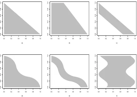
The assumptions (A1), (A2), (A5) and (A6) accommodate a variety of sets I that
arise in real applications. Figure 1 depicts some realistic examples of the set I that
satisfy the assumptions. In particular, those sets of the type in the panels (c) and (e)
satisfy (A2) and (A6) if the maximal vertical or horizontal thickness of the stripe is larger
than the period 1/J of the third component function f3(mJ(·)). In the interpretation
of the examples in Figure 1, we follow the equivalent discussion from Keiding(1990) and
Kuang et al.(2008). The triangle in Figure 1a is typical for insurance or mortality when
none of the underwriting years or cohorts are fully run-off. The standard actuarial term
“fully run-off” means that all events from that underwriting year or cohort have been
observed. In almost all practical cases of estimating outstanding liabilities, actuaries stick
to the triangle format leaving out fully run-off underwriting years. While the triangle also
appears in mortality studies, it is common here to leave the fully run-off cohorts in the
study resulting in the support shape given in Figure 1b. The support in Figure 1c arises
when the data analyst only considers observations from the most recent calendar years.
While this approach is omnipresent in practical actuarial science, there is no formal theory
or mathematical models behind these procedures in the actuarial literature. This paper is
therefore an important step towards formalising mathematically actuarial practise while
at the same time improving it. The support given in Figure 1d and Figure 1e arises
when there is a known time transformation such that time is running at another pace for
well known in mortality studies often coined as versions of accelerated failure time models.
Time transformations are also well known in actuarial science coined as operational time.
However, the academic literature of actuarial science is still struggling to find a formal
definition of what operational time is. This paper offers one potential solution to this
outstanding and important issue. The last Figure 1f is included to give an impression of
the generality of support structures one could deal with inside our model approach. Data
is missing in the beginning and end of the delay period, but the model is still valid and
in-sample forecasts can be constructed.
0.0 0.2 0.4 0.6 0.8 1.0
0.0
0.2
0.4
0.6
0.8
1.0
(a)
0.0 0.2 0.4 0.6 0.8 1.0
0.0
0.2
0.4
0.6
0.8
1.0
(b)
0.0 0.2 0.4 0.6 0.8 1.0
0.0
0.2
0.4
0.6
0.8
1.0
(c)
0.0 0.2 0.4 0.6 0.8 1.0
0.0
0.2
0.4
0.6
0.8
1.0
(d)
0.0 0.2 0.4 0.6 0.8 1.0
0.0
0.2
0.4
0.6
0.8
1.0
(e)
0.0 0.2 0.4 0.6 0.8 1.0
0.0
0.2
0.4
0.6
0.8
1.0
[image:9.612.81.519.295.607.2](f)
Figure 1: Shapes of possible support sets. The horizontal axis indicates the onset (X) and the vertical the development (Y).
the simple multiplicative model. Iff3 above was constant (and therefore not in the model)
then our model reduces to the simple multiplicative model analysed in Mart´ınez-Miranda,
Nielsen, Sperlich and Verrall (2013) and Mammen, Mart´ınez-Miranda and Nielsen (2013).
These two papers point out that the simple multiplicative density forecasting model is a
continuous version of a widely used parametric approach corresponding to a structured
his-togram version of in-sample density forecasting based on the simple multiplicative model.
The in-sample density forecasting model under investigation in this paper generalizes the
simple multiplicative approach in an intuitive and simple way including seasonal effects.
In the following theorem, we show that, if there are two multiplicative representations
of the joint densityf that agree on almost all points inI, then the component functions
also agree on almost all points in [0,1]. We will use this result later in the asymptotic
analysis of our estimation procedure.
Theorem 2 Assume that model (2.1) holds with (A1)–(A3), (A5), (A6). Suppose that
(g1, g2, g3) is a tuple of functions that are bounded away from zero and infinity with R1
0 g1(x)dx = R1
0 g2(y)dy = 1. Let µj = logfj −loggj. Assume that µ1(x) +µ2(y) +
µ3(mJ(x+y)) = 0 a.e. on I. Then µj ≡0 a.e. on [0,1].
3
Methodology
We describe the estimation method for the model (2.1). We first note that the marginal
densities of X, Y and mJ(X +Y) may be zero even if we assume that the joint density
is bounded away from zero. For example, the marginal densities of X and Y at the point
u = 1 are zero for the support set I given in Figure 1a. We estimate the multiplicative
density model on a region where we observe sufficient data. This means that we exclude
the points (1,0) and (0,1) in the estimation in the case of Figure 1a, and the point (1,0)
in the case of Figure 1b. Formally, for a set S ⊂ I, let J1 and J2 denote versions of I1
and I2, respectively, defined byJ1(y) = {x: (x, y)∈S}and J2(x) ={y: (x, y)∈S}, and
and find the largest set S such that
mes(J2(x))≥δ, mes(J1(y))≥δ,
L(J)
X
l=0
mes(J3l(mJ(x+y)))≥δ for all (x, y)∈S,
where mes(A) for a set Adenotes its length. Such a set is given by S ={(x, y) : 0≤x≤
1−δ, 0≤y≤1−δ, x+y≤1}in the case of Figure 1a, andS ={(x, y)∈ I : 0≤x≤1−δ}
in the case of Figure 1b, for example.
We estimate fj on S. Let S1 and S2 be the projections of S onto x- and y-axis,
i.e., S1 = {x ∈ [0,1] : (x, y) ∈ S for some y ∈ [0,1]}, S2 = {y ∈ [0,1] : (x, y) ∈
S for some x ∈ [0,1]}, and S3 = {mJ(x+y) : (x, y) ∈ S}. In the case of Figure 1a,
S1 =S2 = [0,1−δ], S3 = [0,1), but in the case of Figure 1b, S1 = [0,1−δ], S2 = [0,1],
S3 = [0,1). We put the following constraints on fj:
Z
S1
f1(x)dx= Z
S2
f2(y) = 1.
This is only for convenience. Now, we definefw,1(x) = R
J2(x)f(x, y)dy, fw,2(y) =
R
J1(y)f(x, y)dx
andfw,3(z) =
PL(J)
l=0
R
J3l(z)f(x,(z+l)/J−x)dx. Then, the model (2.1) gives the following
integral equations:
fw,1(x) = f1(x) Z
J2(x)
f2(y)f3(mJ(x+y))dy, x∈S1
fw,2(y) = f2(y) Z
J1(y)
f1(x)f3(mJ(x+y))dx, y∈S2
fw,3(z) = f3(z)
L(J)
X
l=0
Z
J3l(z)
f1(x)f2((z+l)/J −x)dx, z ∈S3.
(3.1)
We note that the marginal functions on the left hand sides of the above equations are
bounded away from zero on Sj. Specifically, infu∈Sjfw,j(u) ≥ δinf(x,y)∈If(x, y) > 0 so
that fj in the equations are well-defined.
Suppose that we are given a preliminary estimator of the joint density f. Call it ˆf.
We estimate fw,j by ˆfw,j that are defined as fw,j, respectively, with f being replaced by
the preliminary estimator ˆf. Our proposed estimators of fj, for j = 1,2,3, are obtained
by replacing fw,j in the integral equations (3.1) by ˆfw,j, respectively, and solving the
resulting equations for the multiplicative components. Let ϑ=R
its estimator defined by ˆϑ =n−1Pn
i=1I[(Xi, Yi)∈S]. Putting the constraints
Z
S1
ˆ
f1(x)dx= Z
S2
ˆ
f2(y)dy= 1, Z
S
ˆ
f1(x) ˆf2(y) ˆf3(mJ(x+y))dx dy= ˆϑ, (3.2)
they are given as the solution of the following backfitting equations:
ˆ
f1(x) = ˆθ1·
ˆ
fw,1(x) R
J2(x)
ˆ
f2(y) ˆf3(mJ(x+y))dy
,
ˆ
f2(y) = ˆθ2·
ˆ
fw,2(y) R
J1(y)
ˆ
f1(x) ˆf3(mJ(x+y))dx
,
ˆ
f3(z) = ˆθ3·
ˆ
fw,3(z)
PL(J)
l=0
R
J3l(z)
ˆ
f1(x) ˆf2((z+l)/J −x)dx
,
(3.3)
where ˆθj are chosen so that ˆfj satisfy (3.2).
The solution of (3.3) is not given explicitly. The estimates are calculated by an iterative
algorithm with a starting set of function estimates ˆf1[0] and ˆf2[0] that satisfy the constraints
(3.2). With the initial estimates, we compute ˆf3[0] from the third equation at (3.3). Then,
we update ˆfj[k−1] consecutively forj = 1,2,3 and fork≥1 by the equations at (3.3) until
convergence. Specifically, we compute at the kth cycle (k ≥1) of the iteration
ˆ
f1[k](x) = ˆθ1[k]· fˆw,1(x)
R
J2(x)
ˆ
f2[k−1](y) ˆf3[k−1](mJ(x+y))dy
,
ˆ
f2[k](y) = ˆθ2[k]· fˆw,2(y)
R
J1(y)
ˆ
f1[k](x) ˆf3[k−1](mJ(x+y))dx
,
ˆ
f3[k](z) = ˆθ3[k]· fˆw,3(z)
PL(J)
l=0
R
J3l(z)
ˆ
f1[k](x) ˆf2[k]((z+l)/J −x)dx,
(3.4)
where ˆθ[jk] are chosen so that the resulting ˆfj[k] satisfy (3.2).
We note that the naive two-dimensional kernel density estimator is not consistent near
the boundary region, which jeopardizes the properties of the solution of the backfitting
equation (3.3) at boundaries. For a preliminary estimator ˆf of the joint densityf, we take
local linear estimation technique. The local linear estimator ˆf we consider here is similar
in spirit to the proposal of Cheng (1997). Let a(u, v;x, y) = (1,(u−x)/h1,(v −y)/h2)>
and define
A(x, y) =
Z
S
a(u, v;x, y)a(u, v;x, y)>h−11h−21K
u−x
h1
K
v−y
h2
where (h1, h2) is the bandwidth vector andK is a symmetric univariate probability density
function. Also, define
ˆ
b(x, y) =n−1
n
X
i=1
a(Xi, Yi;x, y)h−11h
−1 2 K
Xi−x
h1
K
Yi−y
h2
Wi,
where Wi = 1 if (Xi, Yi) ∈ S and 0 otherwise. The local linear density estimator ˆf we
consider in this paper is defined by ˆη0, where ˆη = (ˆη0,ηˆ1,ηˆ2) is given by
ˆ
η(x, y) =A(x, y)−1bˆ(x, y). (3.5)
It is alternatively defined as
ˆ
η(x, y) = arg minη lim
b1,b2→0
Z
S
h ˆ
fb1,b2(u, v)−a(u, v;x, y)
>
η(x, y) i2
×K
u−x
h1
K
v−y
h2
du dv,
where ˆfb1,b2 be the standard two-dimensional kernel density estimator defined by
ˆ
fb1,b2(x, y) =n
−1
n
X
i=1
b−11b−21K
x−Xi
b1
K
y−Yi
b2
Wi
for a bandwidth vector (b1, b2).
Before we close this section, we give two remarks. One is that, instead of
integrat-ing the two-dimensional estimator ˆf, one may estimate fw,j directly from the data. In
particular, one may estimatefw,j by the one-dimensional kernel density estimators
˜
fw,1(x) = n−1h−11
n
X
i=1
K
Xi−x
h1
Wi,
˜
fw,2(y) = n−1h−21
n
X
i=1
K
Yi−y
h2
Wi,
˜
fw,3(z) = n−1h−31
n
X
i=1
K
mJ(Xi+Yi)−z
h3
Wi.
Our theory that we present in the next section is valid for this alternative estimation
procedure. The other thing we would like to remark is that one may be also interested in an
extension of the model (2.1) that arises when one observes a covariateUi ∈Rdalong with
of (X, Y) given U=u has the form f(x, y|u) =f1(x,u)f2(y,u)f3(mJ(x+y),u), (x, y)∈
I, where the constraints (B1) now applies to f1(·,z) and f2(·,z) for each z. The method
and theory for this extended model are easy to derive from those we present here.
4
Theoretical Properties
LetS denote the space of function tuplesg = (g1, g2, g3) with square integrable univariate
functions gj in the spaceL2[0,1]. Define nonlinear functionals Fj for 1≤j ≤3 on S by
F1(g) = 1− Z
S1
g1(x)dx,
F2(g) = 1− Z
S2
g2(y)dy,
F3(g) = ϑ− Z
S
g1(x)g2(y)g3(mJ(x+y))dx dy.
Also, define nonlinear functionals Fj for 4≤j ≤6, now onR3× S, by
F4(θ,g)(x) = Z
J2(x)
[θ1f(x, y)−g1(x)g2(y)g3(mJ(x+y))] dy,
F5(θ,g)(y) = Z
J1(y)
[θ2f(x, y)−g1(x)g2(y)g3(mJ(x+y))]dx,
F6(θ,g)(z) =
L(J)
X
l=0
Z
J3l(z)
[θ3f(x,(z+l)/J −x)−g1(x)g2((z+l)/J −x)g3(z)]dx,
where θ = (θ1, θ2, θ3)>. Then, we define a nonlinear operator F : R3× S 7→ R3 × S by
F(θ,g)(x, y, z) = (F1(g),F2(g),F3(g),F4(θ,g)(x),F5(θ,g)(y),F6(θ,g)(z))>.
Now, we define nonlinear functionals ˆFj for 1 ≤ j ≤ 3 on S and ˆFj for 4 ≤ j ≤ 6
on R3 × S as F
j in the above, with the joint density f being replaced by its
estima-tor ˆf and ϑ by ˆϑ. Let ˆF : R3 × S 7→ R3 × S be the nonlinear operator defined by ˆ
F(θ,g)(x, y, z) = ( ˆF1(g),Fˆ2(g),Fˆ3(g),Fˆ4(θ,g)(x),Fˆ5(θ,g)(y),Fˆ6(θ,g)(z))>. Our
esti-mators ˆf = ( ˆf1,fˆ2,fˆ3) along with ˆθ = (ˆθ1,θˆ2,θˆ3) are given as the solution of the equation
ˆ
F( ˆθ,ˆf) = 0. (4.1)
From the definition of the nonlinear operator F, we also get F(1,f) = 0, where 1 =
We consider a theoretical approximation of ˆf. Define a nonlinear operator byG(θ,g) =
F(1+θ,f◦(1+g)), whereg1◦g2 denotes the entry-wise multiplication of the two function
vectors g1 and g2. Then, G(0,0) = 0. Let G0(d,δ) denote the derivative of G(θ,g) at
(θ,g) = (0,0) to the direction (d,δ). We write fw(x, y, z) = (fw,1(x), fw,2(y), fw,3(z))>
and ˆµ(x, y, z) = (ˆµ1(x),µˆ2(y),µˆ3(z))>, where
ˆ
µ1(x) =fw,1(x)−1 Z
J2(x)
h ˆ
f(x, y)−f(x, y) i
dy,
ˆ
µ2(y) =fw,2(y)−1 Z
J1(y)
h ˆ
f(x, y)−f(x, y)i dx,
ˆ
µ3(z) =fw,3(z)−1
L(J)
X
l=0
Z
J3l(z)
h ˆ
f(x,(z+l)/J −x)−f(x,(z+l)/J −x)i dx.
(4.2)
LetG0−1 :
R3× S 7→R3× S denote the inverse ofG0, whose existence we will prove in the
Appendix. We define ¯f = ( ¯f1,f¯2,f¯3) along with ¯θ = (¯θ1,θ¯2,θ¯3) by
¯
θ−1
(¯f −f)/f
=G0−1
0
−fw◦µˆ
, (4.3)
where g1/g2 denotes the entrywise division of the function g1 byg2.
It can be seen that δ = (δ1, δ2, δ3)> = (( ¯f1−f1)/f1,( ¯f2−f2)/f2,( ¯f3−f3)/f3)> along
with d= (d1, d2, d3)>= (¯θ1−1,θ¯2−1,θ¯3−1)> are given as the solution of the following
system of integral equations.
δ1(x) =d1+ ˆµ1(x)− Z
J2(x)
δ2(y)
f(x, y)
fw,1(x)
dy−
Z
J2(x)
δ3(mJ(x+y))
f(x, y)
fw,1(x)
dy, x∈S1
δ2(y) =d2+ ˆµ2(y)− Z
J1(y)
δ1(x)
f(x, y)
fw,2(y)
dx−
Z
J1(y)
δ3(mJ(x+y))
f(x, y)
fw,2(y)
dx, y ∈S2
δ3(z) =d3+ ˆµ3(z)−
L(J)
X
l=0
Z
J3l(z)
δ1(x)
f(x,(z+l)/J −x)
fw,3(z)
dx
−
L(J)
X
l=0
Z
J3l(z)
δ2((z+l)/J −x)
f(x,(z+l)/J −x)
fw,3(z)
subject to the constraints
0 = Z
S1
f1(x)δ1(x)dx
0 = Z
S2
f2(y)δ2(y)dy
0 = Z
S
f(x, y) [δ1(x) +δ2(y) +δ3(mJ(x+y))]dx dy.
(4.5)
In the following theorem, we show that the approximation of ˆf by ¯f is good enough.
In the theorem, we assume that ˆf(x, y) −f(x, y) = Op(εn) uniformly on S for some
nonnegative sequence {εn} that converges to zero as n tends to infinity. For the local
linear estimator ˆf defined by (3.5) with h1 ∼ h2 ∼ n−1/5, we have εn = n−3/10
√
logn.
The theorem tells that the approximation errors of ¯fj for ˆfj are of order Op(n−3/5logn).
In Theorem 4 below, we will show that ¯fj −fj have magnitude of order Op(n−2/5
√
logn)
uniformly onSj. This means that the first-order properties of ˆfj are the same as those of
¯
fj.
Theorem 3 Assume that the conditions of Theorem 2 hold, and that the joint density f
is bounded away from zero and infinity on its supportS with continuous partial derivatives on the interior of S. If fˆ(x, y)−f(x, y) =Op(εn) uniformly for (x, y)∈S, then it holds
that |θˆj −θ¯j|=Op(ε2n) and supu∈Sj|
ˆ
fj(u)−f¯j(u)|=Op(ε2n).
Next, we present the limit distribution of (¯f −f)/f. In the next theorem, we assume
that h1 ∼ c1n−1/5 and h2 ∼ c2n−1/5 for some constants c1, c2 > 0. For such constants,
define
˜
fB(x, y) = 1 2
Z
u2K(u)du
c21 ∂
2
∂x2f(x, y) +c 2 2
∂2
∂y2f(x, y)
. (4.6)
Also, define ˜µBj forj = 1,2,3 as ˆµj at (4.2) with the local linear estimator ˆf being replaced
by ˜fB. In the Appendix, we will show that the asymptotic mean of ( ¯f
j −fj)/fj equals
n−2/5βj, where β = (β1, β2, β3) is the solution of the backfitting equation (4.4) with ˆµ
being replaced by ˜µB. Let ˜fA denote the centered version of the naive two-dimensional
kernel density estimator. Specifically,
˜
fA(x, y) =n−1
n
X
i=1
Here and below, we write Kh(u) = K(u/h)/h. Define ˜µjA for j = 1,2,3 as ˜µBj with ˜fA
taking the role of ˜fB. We will also show that the asymptotic variances of ( ¯f
j −fj)/fj
equal those of ˜µAj, respectively, and that they are given by n−4/5σj2, where
σ12(x) =c1−1fw,1(x)−1 Z
K2(u)du,
σ22(y) =c2−1fw,2(y)−1 Z
K2(u)du,
σ32(z) =c2−1fw,3(z)−1 Z
[K∗K(u)][K ∗K(c1u/c2)]du
=c−11fw,3(z)−1 Z
[K∗K(u)][K ∗K(c2u/c1)]du,
where K∗K denotes the two-fold convolution of the kernel K.
In the discussion of Assumption (A6) in Section 2, we note that (A6) allows a finite
number of jumps in Ij(u) for j = 1,2 and I3l(u) as u changes. These jump points are
actually those where the marginal densities fw,j are discontinuous. At these discontinuity
points the expression of the asymptotic distributions of the estimators is complicate. For
this reason, we consider only those points in the partitions (ajk−1, ajk), 1≤k ≤Lj, for the
asymptotic distribution of ˆfj, where ajk are the points that appear in Assumption (A6).
We denote by Sj,c the resulting subset of Sj after deleting all akj, 1 ≤ k ≤ Lj −1. Note
that fw,j is continuous on Sj,c due to (A6). In the theorem below we also denote by Sjo
the interiors of Sj, j = 1,2,3.
For the limit distribution of ˆfj, we put an additional condition on the support set. To
state the condition, let Jo
2(u1;h2) be a subset of J2(u1) such that v ∈ J2o(u1;h2) if and only if v −h2t ∈ J2(u1) for all t ∈[−1,1]. The set J2o(u1;h2) is inside J2(u1) at a depth
h2. In the following assumption, ajk and κ are the points and the function that appear in
Assumption (A6).
(A7) There exist constants C > 0 and α > 1/2 such that the following statements
hold: (i) for any sequence of positive numbers n, J2o(u1;Cαn) ⊂ J2(u2) for all
u1, u2 ∈(a1k−1, ak1)∩S1 with |u1−u2| ≤n, 1≤k ≤L1;J1o(u1;Cαn)⊂J1(u2) for all
u1, u2 ∈(a2k−1, a 2
k)∩S2 with |u1−u2| ≤n, 1≤k ≤L2; (ii) κ(t)≤C|t|α.
Theorem 4 Assume that (A7) and the conditions of Theorem 3 hold, and that the joint
[−1,1], symmetric and Lipschitz continuous. Let the bandwidths hj satisfy n1/5hj → cj
for some constants cj >0. Then, for fixed pointsuj ∈Sjo∩Sj,c, it holds that n2/5( ¯fj(uj)−
fj(uj))/fj(uj) are jointly asymptotically normal with mean(βj(uj) : 1 ≤j ≤3)and
vari-ance diag(σj(uj) : 1 ≤j ≤ 3). Furthermore, ( ¯fj(uj)−fj(uj))/fj(uj) = Op(n−2/5
√
logn)
uniformly for uj ∈Sj.
Remark 2 In the case where the third component function f3 is constant, i.e., there is
no periodic component, the above theorem continue to hold for the component f1 and f2
without those conditions that pertain to the set S3 and the function f3.
5
Numerical Properties
5.1
Simulation studies
We considered two densities on I = {(x, y) : 0 ≤ x, y ≤ 1, x+y ≤ 1}. Model 1 has
the components f1 ≡ f2 ≡ 1 on [0,1], and f3(u) = c1(sin(2πu) + 3/2), u ∈ [0,1], where
c1 > 0 is chosen to make f(x, y) = f1(x)f2(y)f3(mJ(x+y)) be a density on I. Model
2 has f1(u) = 3/2−u, f2(u) = 5/4−3u2/4 and f3(u) = c2(u3 −3u2/2 +u/2 + 1/2)
for some constant c2 > 0. We took J = 2. We computed our estimates on a grid of
bandwidth choice h1 = h2. For Model 1, we took {0.070 + 0.001×j : 0 ≤ j ≤ 30} in
the range [0.070,0.100], and for Model 2 we chose {0.40 + 0.02×j : 0 ≤ j ≤ 20} in
the range [0.40,0.80]. In both cases, the ranges covered the optimal bandwidths. We
obtained MISEj = E
R1
0[ ˆfj(u)− fj(u)]
2du, ISB
j =
R1
0[Efˆj(u)− fj(u)]
2du and IV
j =
ER1
0[ ˆfj(u)−Efˆj(u)]
2du, for 1 ≤j ≤ 3, based on 100 pseudo samples. The sample sizes
were n = 400 and 1,000, but only the results for n = 400 are reported since the lessons
are the same.
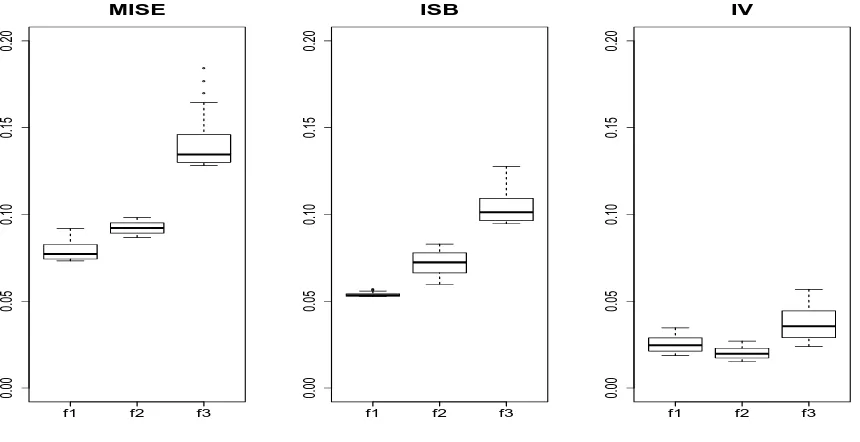
Figure 2 is for Model 1. It shows the boxplots of the values of MISEj, ISBj and
IVj computed using the bandwidths on the grid specified above, and thus gives some
indication of how sensitive our estimators are to the choice of bandwidth. The bandwidth
that gave the minimal value of MISE1+ MISE2+ MISE3 wash1 =h2 = 0.089 in Model 1,
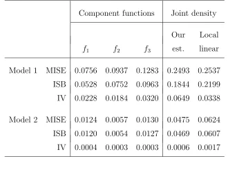
with ISBj and IVj for these optimal bandwidths are reported in Table 1. Although our
primary concern is the estimation of the component functions, it is also of interest to
see how good the produced two-dimensional density estimator ˆf1(x) ˆf2(y) ˆf3(mJ(x+y))
behaves. For this we include in the table the values of MISE, ISB and IV of the
two-dimensional estimates computed using the optimal bandwidthh1 =h2 = 0.089 in Model 1,
and h1 =h2 = 0.64 in Model 2. For comparison, we also report the results for the
two-dimensional local linear estimates defined at (3.5). For the local linear estimator, we used
its optimal choices h1 = h2 = 0.085 in Model 1, and h1 = h2 = 0.48 in Model 2. We
found that the initial local linear estimates had a large portion of mass outsideIand thus
behaved very poorly if they were not re-scaled to be integrated to one onI. The reported
values in Table 1 are for the adjusted local linear estimates. Overall, our two-dimensional
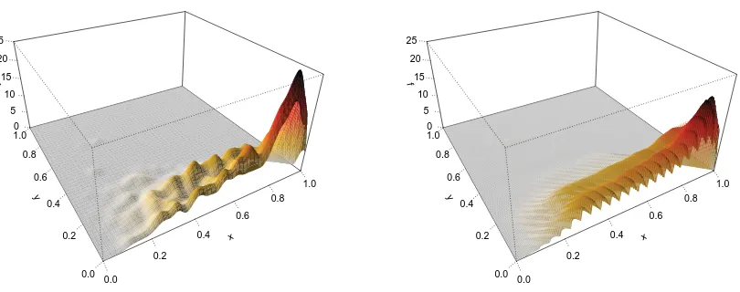
[image:19.612.86.516.402.623.2]estimator has better performance than the local linear estimator, especially in Model 2.
Figure 3 depicts the true density of Model 1 and our two-dimensional estimate that has
the median performance in terms of ISE.
● ● ●
f1 f2 f3
0.00
0.05
0.10
0.15
0.20
MISE
● ●
f1 f2 f3
0.00
0.05
0.10
0.15
0.20
ISB
f1 f2 f3
0.00
0.05
0.10
0.15
0.20
IV
Figure 2: Boxplots for the values of MISE, ISB and IV of our estimates fj computed
Table 1: Mean integrated squared errors (MISE), integrated squared biases (ISB) and integrated
vari-ance (IV) of the estimators.
Component functions Joint density
Our Local
f1 f2 f3 est. linear
Model 1 MISE 0.0756 0.0937 0.1283 0.2493 0.2537
ISB 0.0528 0.0752 0.0963 0.1844 0.2199
IV 0.0228 0.0184 0.0320 0.0649 0.0338
Model 2 MISE 0.0124 0.0057 0.0130 0.0475 0.0624
ISB 0.0120 0.0054 0.0127 0.0469 0.0607
IV 0.0004 0.0003 0.0003 0.0006 0.0017
x
0.0
0.2
0.4
0.6
0.8
y
0.0 0.2
0.4 0.6
0.8
f
0 1 2 3 4 5
x
0.0
0.2
0.4
0.6
0.8
y
0.0 0.2
0.4 0.6
0.8
f
[image:20.612.133.463.149.399.2]0 1 2 3 4 5
Figure 3: The true density (left) and our estimated two-dimensional density function (right) computed from the pseudo sample that gives the median performance in terms of ISE, for Model 1 and n= 400.
5.2
Data examples
[image:20.612.93.502.435.587.2]– and more details about it – is publicly available via the Cass Business School web
site together with the paper “Double Chain Ladder” at the Cass knowledge site. The
observations were the incurred counts of large claims aggregated by months. During
the 264 months 1516 large claims were made. The dataset is provided in the form of a
classical run-off triangle{Nkl: 1≤k, l≤264, k+l ≤265}, whereNkl denotes the number
of large claims incurred in the kth month and reported in the (k +l −1)th month i.e.
with (l−1) months delay. Since the data are grouped monthly, we need pre-smoothing
of the data to apply the model (2.1) that is based on data recorded over a continuous
time scale. A natural way of pre-smoothing is to perturb the data by uniform random
variables. Thus, we converted each claim (k, l) on the two-dimensional discrete time scale
{(k, l) : 1≤k, l ≤264, k+l ≤265}, into (X, Y) on the two-dimensional continuous time
scale I ={(x, y) : 0≤x, y ≤1, x+y≤1}, by
X = k−1 +U1
264 , Y =
l−1 +U2
264 ,
where (U1, U2) is a two-dimensional uniform random variate on the unit square [0,1]2.
This gives a converted dataset {(Xi, Yi) : 1≤ i≤ 1516}. We applied to this dataset our
method of estimating the structured density f of (X, Y).
Since one month corresponds to an interval with length 1/264 on the [0,1] scale, one
year is equivalent to an interval with length 12/264 = 1/22 on the latter scale. We let
the periodic component f3(mJ(·)) in the model (2.1) reflect a possible seasonal effect,
so that we take one year in the real time to be the period of the function. This means
that we let the periodic component f3(mJ(·)) have 1/22 as its period, and thus take
J = 22. For the bandwidth we took h1 = h2 = 0.01. The chosen bandwidth may be
considered to be too small for the estimation off1 andf2. However, we took such a small
bandwidth to detect possible seasonality. Note that the bandwidth size 0.01 corresponds
to 0.01×12×22 = 2.64 months. We found that even with this small bandwidth the
estimated curve ˆf3 was nearly a constant function, which suggests that the large claim
data do not have a seasonal effect.
the dataset by adding a certain level of seasonal effect as follows. We computed
Nkl0 = 2Nkl if k+l = 12mfor somem= 1,2, . . . ,
Nkl0 = 3Nkl if k+l = 12m+ 1 for some m= 1,2, . . . ,
Nkl0 = 5Nkl if k+l = 12m+ 2 for some m= 0,1, . . . ,
Nkl0 = 3Nkl if k+l = 12m+ 3 for some m= 0,1, . . . ,
Nkl0 =Nkl otherwise.
Since (k +l−1 modulo 12) is the actual month of the claims reported, the augmented
dataset has added claims in November, December, January and February. The
augmen-tation resulted in increasing the total number of claims to 2606 from 1516. The increased
counts of reported claims were 252 from 126 for November, 600 from 200 for December,
455 from 91 for January, and 300 from 100 for February.
In our estimation procedure, the bandwidths h1 and h2 control the smoothness of the
local linear estimate ˆf along the x- andy-axis, respectively. Consequently, choosing small
values forh1andh2would result in non-smooth estimates of the functionsf1andf2, which
we observed in the pilot study with h1 =h2 = 0.01. Nevertheless, in some cases setting
these bandwidths to be small, relative to the scales of X and Y, might be preferred when
one needs to detect possible seasonality, as is the case with the current dataset. In our
dataset the bandwidth size 1/264 = 0.0038 on the scale of [0,1] corresponds to one month
in real time. Thus, taking the bandwidths to be 0.015, for example, that corresponds to
a period of four months, forces the seasonal effect to almost vanish in the estimate of f3.
To achieve both aims of producing smooth estimates of f1 and f2, and of detecting
possible seasonal effect, we applied to the augmented dataset a two-stage procedure that
is based on our estimation method described in Section 3. In the first stage, we got a local
linear estimate ˆf with h1 = h2 = 0.01, and found an estimate of f3 using the iteration
scheme at (3.4). In the second stage, we recomputed a local linear estimate ˆf with larger
bandwidths h1 = h2 = 0.05, and found estimates of f1 and f2 using only the first two
updating equations at (3.4) with ˆf3[k−1] being replaced by the estimate of f3 obtained in
the first stage.
pre-sented in Figure 4. Clearly, the seasonal effect of the augmented dataset was well recovered
in the estimate of f3, and at the same time smooth estimates of f1 and f2 were produced.
The augmented data set indicate an increased number of claims in the winter time. This
is clearly reflected in the estimated results, where the first part and the last part of the
estimated effect is higher than the rest of the curve. Imagine the realistic situation that
a non-life insurer on the first day of November has to produce budget expenses for the
rest of the year. The classical multiplicative methodology is not able to reflect the two
month perspective of such a budget. Therefore considerable work is being done manually
in Finance and Actuarial departments of non-life insurance companies to correct for such
effects. With our new seasonal correction costly manual procedures can be replaced by
cost saving automatic ones eventually benefitting the prices all of us as end customers
have to pay for insurance products.
Figure 5 depicts the resulting dimensional joint density. Notice that this
two-dimensional density is clearly non-multiplicative. The seasonal correction provides a
vi-sually deviation from the multiplicative shape. Also, note that while this two-dimensional
density is non-multiplicative, the nature of this deviation is not immediately clear to the
eye. Whether the deviation is pure noise, a seasonal effect or some other effect is not easy
to get from the full two-dimensional graph of the local linear density estimate which is
also presented in Figure 5. For the local linear estimate we usedh1 =h2 = 0.03. We tried
other bandwidth choices such as 0.01 and 0.05, but found that the smaller one gave too
rough estimate and the larger one produced too smooth a surface. Our two-dimensional
density estimate therefore illustrates why research into structured densities on non-trivial
supports is crucial to extract information beyond the classical and simple multiplicative
0.0 0.2 0.4 0.6 0.8 1.0
02468
x
hat f1
0.0 0.2 0.4 0.6 0.8 1.0
02468
y
hat f2
0.0 0.2 0.4 0.6 0.8 1.0
02468
z
[image:24.612.75.515.109.294.2]hat f3
Figure 4: Estimated curves fˆj for the model (2.1) obtained by applying the two-stage
procedure to the augmented large claim data.
x
0.0 0.2
0.4 0.6
0.8 1.0
y
0.0 0.2 0.4 0.6 0.8 1.0
f
0 5 10 15 20 25
x
0.0 0.2
0.4 0.6
0.8 1.0
y
0.0 0.2 0.4 0.6 0.8 1.0
f
0 5 10 15 20 25
Figure 5: Local linear joint density estimate (left) and our estimate (right) for the model (2.1) obtained by applying the two-stage procedure to the augmented large claim data
Appendix
A.1
Proof of Theorem 1
Suppose that (g1, g2, g3) is a tuple of functions that are bounded away from zero and
infinity withR01g1(x)dx= R1
[image:24.612.100.505.405.565.2]Furthermore, we assume that g1 and g2 are differentiable on [0,1] and that g3 is twice
differentiable on [0,1). For j ∈ {1,2,3} define µj = logfj −loggj. By assumption we
have
µ1(x) +µ2(y) +µ3(mJ(x+y)) = 0.
For z ∈[0,1) we choose (x, y) in the interior of I with mJ(x+y) =z. Then we have
that
0 = ∂ 2
∂x∂y[µ1(x) +µ2(y) +µ3(mJ(x+y))] =µ
00
3(z).
Thus µ3 is a linear function. Furthermore, we have that µ3(0) = µ3(1−). This follows
by noting that µ3(0) = −µ1(x)−µ2(y) for (x, y) ∈ I with mJ(x+y) = 0. Note that
mJ(x+y) = 0 if and only if x+y =l/J for some l ≥ 1, if (x, y) is in the interior of I.
After slightly decreasing x and y to x+δx and y+δy with small δx <0, δy <0 we have
thatµ3(1 +J(δx+δy)) =−µ1(x+δx)−µ2(y+δy) sincemJ(x+y+δx+δy) = 1 +J(δx+δy).
Thusµ3(0) =µ3(1−) follows from continuity of µ1 and µ2. We conclude that µ3 must be
a constant function. Thus µ1(x) +µ2(y) is a constant function.
From Assumption (A5) we get that µ1(x) is constant on the intervals [xj, xj+1].
Be-cause the union of these intervals is equal to [0,1] we conclude that µ1(x) is constant on
[0,1]. Using again (A5) we get thatµ2(y) is constant on [0,1]. Because of the assumption
that R1
0 g1(x)dx= R1
0 g2(y)dy= 1 and R1
0 f1(x)dx= R1
0 f2(y)dy = 1 we get thatf1 =g1,
f2 =g2 and f3 =g3. This concludes the proof.
A.2
Proof of Theorem 2
We first argue thatµ1,µ2 andµ3 are a.e. equal to piecewise continuous functions on (0,1),
with a finite number of pieces. To see that µ1 is a.e. equal to a piecewise continuous
function, we note that
µ1(x) =− Z
I2(x)
[µ2(y) +µ3(mJ(x+y))] dy/mes(I2(x)), a.e. x∈(0,1).
Here, because of (A3) and (A6), the right hand side is a piecewise continuous function.
Thus, µ1 is a.e. equal to a piecewise continuous function. In abuse of notation, we now
µ2, and µ3 are piecewise continuous functions (or more precisely a.e. equal to piecewise
continuous functions). This implies that
µ1(x) +µ2(y) +µ3(mJ(x+y)) = 0 (A.1)
for (x, y, mJ(x+y))6∈ {x1, ..., xr1}×(0,1)
2∪(0,1)×{y
1, ..., yr2}×(0,1)∪(0,1)
2×{z
1, ..., zr3}
for some values x1, ..., xr1, y1, ..., yr2, z1, ..., zr3 ∈(0,1).
We now argue thatµ3 is continuous on [0,1). To see thatµ3 is continuous atz0 ∈[0,1),
we choose (x0, y0) in the interior ofI such thatmJ(x0+y0) =z0. This is possible because
of Assumption (A2). We can choose x0 and y0 such that µ1 is continuous at x0 and µ2
is continuous at y0. Thus we get from (A.1) that µ3 is continuous at z0. Similarly one
shows thatµ1 and µ2 are continuous functions on [0,1]. This gives that
µ1(x) +µ2(y) +µ3(mJ(x+y)) = 0 (A.2)
for all x, y ∈(0,1).
For z0 ∈ [0,1) we choose (x0, y0) in the interior of I with mJ(x0 +y0) = z0. Note
that for δx and δy sufficiently small we get for z0 ∈ (0,1) that mJ(x0 +δx +y0 +δy) =
z0+J(δx+δy). This gives forδx and δy sufficiently small that
µ1(x0+δx) +µ2(y0+δy) +µ3(z0+J(δx+δy)) = 0.
Withδx, δ0y and δy sufficiently small we get that
µ2(y0+δy) +µ3(z0+J(δx+δy)) = µ2(y0+δy0) +µ3(z0+J(δx+δ0y)).
With the special choice δx =−δy this gives
µ2(y0+δy) +µ3(z0) =µ2(y0+δ0y) +µ3(z0+J(δ0y−δy)).
Letγ be a function defined by γ(u) = µ3(z0+J u)−µ3(z0). From the last two equations
taking u=δx+δy and v =δ0y−δy, we get
γ(u+v) =γ(u) +γ(v)
foru, v sufficiently small. This implies that, with a constantcz0 depending onz0 we have
µ3(z) = az0+bz0z with constants az0 and bz0 depending on z0 for z in a neighborhood Uz0
of z0. Because every interval [z0, z00] with 0< z0 < z00 <1 can be covered by the union of
finitely many Uz’s we get that for each such interval it holds that µ3(z) = az0,z00 +bz0,z00z
for z ∈[z0, z00] with constants az0,z00 and bz0,z00 depending on the chosen interval [z0, z00].
One can repeat the above arguments for z0 = 0. Then we have thatmJ(x0+δx+y0+
δy) = 1 +J(δx+δy) for δx+δy <0 andmJ(x0+δx+y0+δy) = J(δx+δy) for δx+δy >0.
Arguing as above with δx +δy > 0 and δy0 −δy > 0 we get that µ3(z) = a+ +b+z for
z ∈(0, z+] forz+ >0 small enough with some constants a+ and b+. Similarly we get by
choosingδx+δy <0 andδy0 −δy <0 thatµ3(z) =a−+b−z forz ∈(z−,1) forz− <1 large
enough with some constants a− and b−. Thus we get that µ3(z) = a+bz for z ∈ (0,1)
with some constants a and b.
Furthermore, using continuity of µ1, µ2 and the relation µ3(mJ(x+y)) = −µ1(x)−
µ2(y) for z = mJ(x+y) with z in (1−δ,1) and (0, δ) with δ > 0 small enough we get
thatµ3(0) =µ3(1−). Thus we haveb = 0 and we conclude thatµ3 is a constant function.
This gives
µ1(x) +µ2(y) =−a
for all (x, y)∈ I. Now arguing as in the proof of Theorem 1 we get that f1 =g1,f2 =g2
and f3 =g3. This concludes the proof.
A.3
Proof of Theorem 3
Let G0(θ,g)(d,δ) denote the derivative G, defined in Section 4, at (θ,g) to the direction
(d,δ). We note that we write G0(0,0)(d,δ) simply as G0(d,δ) in Section 4. We use the
sup-norm k(d,δ)k∞ as a metric in the space R3× S, defined by
k(d,δ)k∞= maxn|d1|,|d2|,|d3|,sup
u∈S1
|δ1(u)|,sup
u∈S2
|δ2(u)|,sup
u∈S3
|δ3(u)| o
.
Define ˆG(θ,g) = ˆF(1+θ,f ◦(1+g)), where ˆF is defined in Section 4, and let ˆG0(θ,g)
denote the derivative of ˆG at (θ,g). In the setting where ˆf(x, y) −f(x, y) = Op(εn)
uniformly for (x, y)∈ I, we claim
(i) supk(d,δ)k∞=1kGˆ0(0,0)(d,δ)− G0(0,0)(d,δ)k
(ii) The operator G0(0,0) is invertible and has bounded inverse;
(iii) The operator ˆG0 is Lipschitz continuous with probability tending to one, i.e., there
exists constants r, C >0 such that, with probability tending to one,
sup
k(d,δ)k∞=1
kGˆ0(θ1,g1)(d,δ)−Gˆ0(θ2,g2)(d,δ)k∞≤Ck(θ1,g1)−(θ2,g2)k∞
for all (θ1,g1), (θ2,g2) ∈ Br(0,0), where Br(θ,g) is a ball with radius r > 0 in
R3× S centered at (θ,g).
Theorem 3 basically follows from the above (i)–(iii). To prove the theorem using (i)–
(iii), we note that Claim (ii) with the definitions of ¯θ and ¯f at (4.3) gives ¯θ−1=Op(εn)
and (¯f −f)/f =Op(εn). With (i) and (iii), this implies that
sup
k(d,δ)k∞=1
kGˆ0( ¯θ−1,(¯f −f)/f)(d,δ)− G0(0,0)(d,δ)k=Op(εn). (A.3)
Now, from (ii) it follows that there exists a constant C > 0 such that the map ˆG0( ¯θ−
1,(¯f−f)/f) is invertible andkGˆ0( ¯θ−1,(¯f−f)/f)−1(d,δ)k∞ ≤Ck(d,δ)k∞with probability
tending to one. Also, (iii) is valid for all (θ1,g1), (θ2,g2)∈B2r( ¯θ−1,(¯f −f)/f). Then,
we can argue that the solution of the equation ˆG(θ,g) = 0, which is ( ˆθ−1,(ˆf −f)/f),
is within Cαn distance from ( ¯θ −1,(¯f −f)/f), with probability tending to one, where
C >0 is a constant and αn =kGˆ( ¯θ−1,(¯f−f)/f)k∞. This follows from an application of
Newton-Kantorovich theorem, see Deimling (1985) or Yu, Park and Mammen (2008) for
a statement of the theorem and related applications. To compute αn we note that
ˆ
G( ¯θ−1,(¯f −f)/f) = ˆG(0,0) + ˆG0(0,0)( ¯θ−1,(¯f −f)/f) +Op(ε2n)
= ˆG(0,0) +G0(0,0)( ¯θ−1,(¯f −f)/f) +Op(ε2n).
(A.4)
For the first equation of (A.4) we have used (iii) and the facts that ¯θ−1= Op(εn) and
(¯f −f)/f =Op(εn). The second equation of (A.4) follows from the inequality
kGˆ0(0,0)(d,δ)− G0(0,0)(d,δ)k∞≤C sup
x,y∈S
|fˆ(x, y)−f(x, y)| · k(d,δ)k∞
for some constantC > 0. Now, ˆG(0,0) = ˆF(1,f) = (0>,(fw◦µˆ)>)>. From the definition
(4.3), we also getG0(0,0)( ¯θ−1,(¯f−f)/f) = (0>,−(f
w◦µˆ)>)>. This provesαn =Op(ε2n),
Claim (i) follows from the uniform convergence of ˆf to f that is assumed in the
theorem: sup(x,y)∈S|fˆ(x, y)−f(x, y)|= Op(εn). Below, we give the proofs of Claims (ii)
and (iii).
Proof of Claim (ii). For this claim we first prove that the map G0(0,0) is one-to-one.
Suppose that G0(0,0)(d,δ) = 0for some d= (d
1, d2, d3)> and δ = (δ1, δ2, δ3)>. Then, by integrating the fourth component ofG0(0,0)(d,δ), we find that
0 = Z
S
f(x, y)[δ1(x) +δ2(y) +δ3(mJ(x+y))]dx dy =d1 Z
S
f(x, y)dx dy,
where the first equation holds since the right hand side equals, up to sign change, the third
component of G0(0,0)(d,δ). Similarly, we getd
2 =d3 = 0. Now, from G0(0,0)(0,δ) =0 we have
0 = Z
S1×S2×S3
(0>,δ(x, y, z)>)G0(0,δ)(x, y, z)dx dy dz
=−
Z
S
f(x, y)[δ1(x) +δ2(y) +δ3(mJ(x+y))]2dx dy.
This implies
δ1(x) +δ2(y) +δ3(mJ(x+y)) = 0 a.e. on S. (A.5)
Arguing as in the proof of Theorem 2 using the last three equations ofG0(0,0)(0,δ) =0,
we obtainδj ≡0 on Sj, 1≤j ≤3.
Next, we prove that the map G0(0,0) is onto. For a tuple (c,η) with c= (c
1, c2, c3)> and η(x, y, z) = (η1(x), η2(y), η(z))>, suppose that h(c,η),G0(0,0)(d,δ)i = 0 for all
(d,δ)∈R3× S. This implies
0 = Z
S
f(x, y)η1(x)dx dy,
0 = Z
S
f(x, y)η2(y)dx dy,
0 = Z
S
f(x, y)η3(mJ(x+y))dx dy,
0 = Z
J2(x)
f(x, y)[η1(x) +η2(y) +η3(mJ(x+y))]dy+c1f1(x) +c3fw,1(x),
0 = Z
J1(y)
f(x, y)[η1(x) +η2(y) +η3(mJ(x+y))]dx+c2f2(y) +c3fw,2(y),
0 =
L(J)
X
l=0
Z
J3l(z)
From the first three equations of (A.6), we get c1 +ϑc3 = 0 by integrating the fourth
equation. Similarly, we obtain c2 +ϑc3 = 0 and c3 = 0 by integrating the fifth and the
sixth equations. This establishes c1 =c2 =c3 = 0. Putting back these constant values to
(A.6), multiplying η1(x), η2(y) and η3(z) to the right hand sides of the fourth, fifth and
sixth equations, respectively, and then integrating them give
Z
S
f(x, y)[η1(x) +η2(y) +η3(mJ(x+y))]2dx dy= 0.
Going through the arguments in the proof ofG0(0,0) being one-to-one and now using the
first two equations of (A.6) give η1 =η2 =η3 ≡0. Note that the first two equations can
be written as RS
1fw,1(x)η1(x)dx = 0 and
R
S2fw,2(y)η2(y)dy = 0, and thus in the latter
proof fw,j for j = 1,2 take the roles of fj in the former proof. The foregoing arguments
show that (0,0) is the only tuple that is perpendicular to the range space of G0(0,0),
which implies that G0(0,0) is onto.
To verify that the inverse mapG0(0,0)−1 is bounded, it suffices to prove that the
bijec-tive linear operator G0(0,0) is bounded, owing to the bounded inverse theorem. Indeed,
it holds that there exists a constant C > 0 such that kG0(0,0)(d,δ)k∞ ≤ Ck(d,δ)k∞.
This completes the proof of Claim (ii).
Proof of Claim (iii). We first note that ˆG0(θ
1,g1)(d,δ)−Gˆ0(θ2,g2)(d,δ) = G0(θ1,g1)(d,δ)−
G0(θ
2,g2)(d,δ). From this, we get that, for each given r >0
kGˆ0(θ1,g1)(d,δ)−Gˆ0(θ2,g2)(d,δ)k∞≤6 (1 +r) max 1≤j≤3usup∈S
j
fw,j(u)kg2−g1k∞
for all (θ1,g1), (θ2,g2)∈Br(0,0) and for all (d,δ) withk(d,δ)k∞ = 1. For this, we used
the inequality
sup
(x,y,z)∈S1×S2×S3
|κ(x, y, z;g2,δ)−κ(x, y, z;g1,δ)| ≤3kδk∞(2 +kg1k∞+kg2k∞)kg2−g1k∞.
This completes the proof of (iii).
A.4
Proof of Theorem 4
Let ˆfA(x, y) be the first entry of ˆηA(x, y), where ˆηA is defined as ˆη at (3.5) with ˆb being
(f(x, y), h1∂f(x, y)/∂x, h2∂f(x, y)/∂y)>. Then, ˆf(x, y) = f(x, y) + ˆfA(x, y) + ˆfB(x, y).
Define ˆµA and ˆµB as ˆµ at (4.2) with ˆf −f being replaced by ˆfA and ˆfB, respectively,
and ¯fs/f = ( ¯f1s/f1,f¯2s/f2,f¯3s/f3) along with ¯θs−1= (¯θ1s−1,θ¯s2−1,θ¯3s−1) fors =A and
B as the solution of the backfitting equation (4.4) with ˆµ being replaced by ˆµs, subject
to the constraints (4.5). Since the backfitting equation (4.4) is linear in ˆµ, we get that
¯
f =f + ¯fA+ ¯fB and ¯θ = ¯θA−1+ ¯θB.
For simplicity, write the backfitting equation (4.4) as δ = d+ ˆµ−Tδ with an
ap-propriate definition of the linear operator T. From the definitions of ¯fA and ¯θA we have ¯
fA/f = ¯θA−1+ ˆµA−T(¯fA/f). From Lemma 2 below, we obtain
¯fA/f −µˆA = ¯θA−1−T(¯fA/f −µˆA) +o
p(n−2/5)
uniformly onS1×S2×S3. This implies ¯fA/f−µˆA=op(n−2/5) uniformly onS1×S2×S3
and ¯θA−1=o
p(n−2/5).
Now, for the deterministic part ¯fB, recall the definitions of ˜fB and ˜µB at (4.6) and
thereafter, respectively. Letrn= ˆµB−n−2/5µ˜B. According to Lemma 2,rn=o(n−2/5) on
S10 ×S20 ×S30, where Sj0 is a subset of Sj with the property that mes(Sj−Sj0) = O(n
−1/5).
We also get rn=O(n−2/5) on S1×S2×S3. This impliesT(rn) = o(n−2/5), so that
¯
fB/f −rn = ¯θB−1+n−2/5µ˜B−T(¯fB/f −rn) +op(n−2/5)
uniformly on S1 ×S2×S3. Thus, (¯fB/f,θ¯B−1) equals the solution of the backfitting
equation δ = d+n−2/5µ˜B −Tδ, up to an additive term whose jth component has a
magnitude of an order o(n−2/5) on S0
j and O(n
−2/5) on the whole setS
j.
The asymptotic distribution of ( ¯fj(uj)−fj(uj))/fj(uj) : 1≤j ≤3
for fixed uj ∈
Sj,c∩Sjo is then readily obtained from the above results. The asymptotic mean is given as
the solution (δj(uj) : 1 ≤j ≤3) of the backfitting equation (4.4) with ˆµj being replaced
by n−2/5µ˜B
those of ˜µAj, where
˜
µA1(x) = fw,1(x)−1 Z
J2(x)
˜
fA(x, y)dy,
˜
µA2(y) = fw,2(y)−1 Z
J1(y)
˜
fA(x, y)dx,
˜
µA3(z) = fw,3(z)−1
L(J)
X
l=0
Z
J3l(z)
˜
fA(x,(z+l)/J −x)dx
and ˜fA(x, y) = n−1Pn
i=1[Kh1(Xi−x)Kh2(Yi−y)Wi−E(Kh1(Xi−x)Kh2(Yi−y)Wi)].
This is due to (A.9), (A.10) and the corresponding property for ˆµA3 in the proof of Lemma 2
below.
To compute var(˜µA
1(u1)), we note that, due to the assumption (A7) and thus from Lemma 1, we may find constants C > 0 and α > 1/2 such that J2o(u;Chα1 +h2) ⊂
Jo
2(u1;h2) for alluwith|u−u1| ≤h1, ifnis sufficiently large. Note thatJ2o(u;Chα1+h2) is insideJ2o(u;h2) at a depthCh1α. Then, it can be shown that, for all (u, v) with|u−u1| ≤h1
and v ∈Jo
2(u;Chα1 +h2), the set {(v−y)/h2 :y∈J2(u1)} covers the interval [−1,1], the support of the kernelK. This implies thatKh1(u−u1)ν(u1, v) = Kh1(u−u1) for all (u, v)
with |u−u1| ≤h1 and v ∈J2o(u;Chα1 +h2), where ν(u1, v) = R
J2(u1)Kh2(v−y)dy. Using
this and the fact that the Lebesgue measure of the set difference J2(u)−J2o(u;Chα1 +h2)
has a magnitude of order n−min{1,α}/5, we get
var(˜µA1(u1)) = fw,1(u1)−2n−1h−11 Z S 1 h1 K
u−u1
h1 2
ν(u1, v)2f(u, v)du dv+O(n−1)
=fw,1(u1)−2n−1h−11 Z
|u−u1|≤h1
Z
Jo
2(u;Chα1+h2)
1
h1
K
u−u1
h1 2
ν(u1, v)2
× f(u, v)dv du+o(n−1h−1)
=fw,1(u1)−2n−1h−11 Z S 1 h1 K
u−u1
h1 2
f(u, v)du dv+o(n−1h−1)
=n−1h−11fw,1(u1)−1 Z
K2(u)du+o(n−1h−1).
The last equation holds since u1 ∈ S1,c, so that fw,1 is continuous at u1, and it is a fixed
point in the interior of S1. Similarly, we obtain
var(˜µA2(u2)) =n−1h2−1fw,2(u2)−1 Z
The calculation of the asymptotic variance of ˜µA3(u3) is more involved than those of
var(˜µA
j (uj)) for j = 1,2. For this, we observe that, ifl 6=l0, then for any given z ∈[0,1]
and (u, v)∈ I we have
πl,l0(z, u, v, x, x0)
≡Kh1(u−x)Kh2
v−z+l
J +x
Kh1(u−x
0
)Kh2
v−z+l 0
J +x
0
= 0
for all x, x0 except the case (z+l)/J −x= (z+l0)/J −x0, ifn is sufficiently large. This
implies that
var(˜µA3(u3)) =fw,3(u3)−2n−1
L(J)
X
l=0
Z
J3l(u3)
Z
J3l(u3)
Z
S
πl(u3, u, v, x, x0)f(u, v)du dv dx dx0
+O(n−1),
where πl = πl,l. From Lemma 1 again, we may find constants C > 0 and α > 1/2 such
thatJo
2(x;Chα1+h2)⊂J2o(u;h2) for allx, u∈(a1k−1, a1k)∩S1 with|u−x| ≤h1, 1 ≤k≤L1. Define a subsetJ30l(u3) of [0,1] such thatx∈J30l(u3) if and only ifx∈J3l(u3+J(h2+Chα1)t)
for all t ∈[−1,1]. Then, for a givenu∈S1,c, it follows that
[−1,1]⊂
v−(u3+l)/J +x
h2
:v ∈J2(u)
for all x ∈ J30l(u3) such that |x −u| ≤ h1 and x lies in the same partition (a1k−1, a 1
k)
as u. This holds since x ∈ J3l(z) implies (z +l)/J −x ∈ J2(x). This entails that, for
x∈J30l(u3)∩S1o,c(h1),
Z
S
πl(u3, u, v, x, x0)du dv
= Z
[−1,1]2
K(t)K(s)h−11K
t+ x−x
0
h1
h−21K
s+x
0−x
h2
dt ds
= (K∗K)h1(x−x
0
)(K∗K)h2(x−x
0
),
where K ∗K denotes the convolution of K defined by K ∗K(u) = R K(t)K(t +u)dt.
Here and below, So
j,c(h) for a small number h > 0 denotes the set of x ∈ Sj,c such that