Neural-Symbolic Monitoring and Adaptation

City, University of London Institutional Repository

Citation

:

Perotti, A., d'Avila Garcez, A. S. and Boella, G. (2015). Neural-Symbolic

Monitoring and Adaptation. In: Proceedings of the IEEE International Joint Conference on

Neural Networks (IJCNN 2015). (pp. 1-8). IEEE.

This is the accepted version of the paper.

This version of the publication may differ from the final published

version.

Permanent repository link:

http://openaccess.city.ac.uk/id/eprint/11909/

Link to published version

:

http://dx.doi.org/10.1109/IJCNN.2015.7280713

Copyright and reuse:

City Research Online aims to make research

outputs of City, University of London available to a wider audience.

Copyright and Moral Rights remain with the author(s) and/or copyright

holders. URLs from City Research Online may be freely distributed and

linked to.

City Research Online: http://openaccess.city.ac.uk/ publications@city.ac.uk

Neural-Symbolic Monitoring and Adaptation

Alan Perotti

Artur d’Avila Garcez

Guido Boella

Abstract—Runtime monitors check the execution of a system under scrutiny against a set of formal specifications describing a prescribed behaviour. The two core properties for monitoring systems are scalability and adaptability. In this paper we show how RuleRunner, our previous neural-symbolic monitoring sys-tem, can exploit learning strategies in order to integrate desired deviations with the initial set of specification. The resulting system allows for fast conformance checking and can suggest possible enhanced models when the initial set of specifications has to be adapted in order to include new patterns.

I. INTRODUCTION

The expanding capabilities of information systems and other frameworks that depend on computing resulted in a spectacular growth of the ”digital universe” (i.e., all data stored and/or exchanged electronically). It is essential to continuously monitor the execution of data-producing systems, as well-timed fault detection can prevent a number of undesired malfunctions and breakdowns.

A first requirement for runtime verification systems is scal-ability, as this guarantees efficiency when dealing with big data or systems with limited computational resources. In [13] we introduced RuleRunner, a novel rule-based runtime verification system designed to check the satisfiability of temporal properties over finite traces of events, and showed how to encode it into a standard connectionist model. The resulting neural monitors benefit from sparse form representation and parallel (GPU) computation to improve the monitoring performance.

In this paper we tackle another crucial requirement for run-time monitoring systems: adaptability. Adaptability overcomes the standard classification approach to monitoring (where the verification task simply labels a trace as complying or not) and allows a monitor to adapt to new models or include unexpected exceptions.

In the Business Process area, a more flexible approach to monitoring is offered by model enhancement, where an initial model can be refined to better suit iterative development cycles and to capture a system’sconcept drift. It may be the case that a user or domain expert would like to modify the verdict of a monitoring task.

In other scenarios, such as the implementation of directives in big companies like banks, the task execution may differ from the rigid protocol enforcement, due to obstacles (from broken printers to strikes) or by adaptations to specific needs (dynamic resources reallocation). If the actual process execution represents an improvement in terms of efficiency, it is relevant to adapt the original process model in order to capture and formalise the system’s behaviour.

We remark that this task differs frompattern discovery, as it does not infer an ex-novo model from the observed traces: the

desired feature is to be able to adapt the existing model. We therefore propose a framework (visualised in Figure 1) based on our RuleRunner system and integrating temporal logic and neural networks, for online monitoring and property adaptation.

Monitoring (Reasoning)

Adaptation (Learning)

actual != desired ? Specification

Labelled Trace Symbolic Encoding

Neural Encoding

Verdict

RuleRunner

Fig. 1: General framework

An initial temporal specification (i.e., one or more prop-erties) is provided as the expected behaviour of the system in analysis. A runtime verification system, monitoring that property, is then built. In Figure 1 we have stressed how in our case the encoding is decomposed in two steps. This is a pre-processing phase: the verification system is built once and can then be used, at run time, to monitor traces. The monitoring process determines whether the pattern of these operations violates the specified property, providing binary verdicts. The sub-workflow framed in a dashed line represents the monitoring task as performed by RuleRunner. If the domain expert deems some traces to be misclassified, the monitor enters an off-line learning phase, where it modifies the encoded property in order to modified the verdict for the traces marked as misclassified. The result of the learning process should be available both as a ready-to-use monitor and as a logical formula describing the new adapted property, thus creating an iterative development cycle.

II. TECHNICALBACKGROUND

A. Runtime Verification

The broad subject of verification comprises all techniques suitable for showing that a system satisfies its specification(s). Correctness properties in verification specify all admissible individual executions of a system and are usually formulated in some variant of linear temporal logic ([14]). LTL properties are checked against real systems through a process called model checking: more formally, given a model of a system and a formal specification, the model checking problem requires to exhaustively and automatically check whether the model meets the specification: however, software model checking is often computationally hard [7], and infeasible when the model of the observed system is not known. A practical alternative is to monitor the running program, and check on the fly whether desired temporal properties hold: Runtime Verification [12], based on the concept of execution analysis, aims to be a lightweight verification technique complementing other verifi-cation techniques such as model checking. Runtime monitoring is a valid option when the program must run in an environment that needs to keep track for violations of the specification, but the source code is unavailable for inspection for proprietary reasons or due to outsourcing. There exist several RV systems, and they can be clustered in three main approaches, based respectively on rewriting [16], [18] [10], automata [7], [6] [9] and rules [1] [13]. The aforementioned restrictions rule out several classical model-checking approaches, based on the construction of a model of the analysed system: for runtime verification, one has to rely on the analysis of the so-called

traces. Traces are streams of events, discretised according to some temporal granularity: each discrete component of a trace is called cell, and it includes a set ofevents, orobservations, occurred in a given time span.

B. Neural-symbolic Integration

(Artificial) Neural Networks [11] are computational models inspired by biological nervous systems and generally presented as systems of interconnected ‘neurons’ which can compute values from inputs. The Neural-Symbolic Integration area provides several hybrid systems that combine symbolical and sub-symbolical paradigms in an integrated effort. A milestone in neural-symbolic integration is the the Connectionist Inductive Learning and Logic Programming (CILP) system [5]. CILP’s Translation Algorithm maps a general logic programP into a single-hidden-layer neural network N such thatN computes the least fixed-point of P. In particular, rules are mapped onto hidden neurons, the preconditions of rules onto input neurons and the conclusion of the rules onto output neurons. The weights are then adjusted to express the dependence among all these elements. The obtained network implements a massively parallel model for Logic Programming, and it can perform inductive learning from examples, by means of standard learning strategies.

Borges et. al [3] proposed a new neural-symbolic system, named Sequential Connectionist Temporal Logic (SCTL) for integrating verification and adaptation of software descriptions. This framework encodes a system description into a particular kind of network, namely NARX (Nonlinear AutoRegressive with eXogenous inputs, [17]) and then a learning phase allows the integration of different knowledge sources. Properties to be

satisfied are checked by means of an external model checking tool (such as NuSMV [4]): if a property is not satisfied, the tool provides a counterexample that can be adapted with the help of an expert and be used to train the NARX network to adapt the model.

III. RULERUNNER

In a nutshell, RuleRunner [13] is a neural-symbolic system where an LTL monitor is translated in a standard, feedfor-ward neural network. The monitor is initially computed as a purely symbolic system, composed by rules encoding the LTL operators, and then encoded in a standard recurrent neural network. As a result of the neural encoding, the monitoring task corresponds to a feedforward recurrent activation of the neural network encoding the monitor.

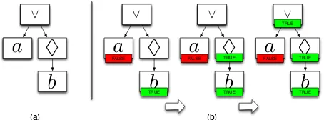
Given an LTL formula φ, RuleRunner is based on the parsing tree of φ: this is a tree where each node corresponds to an operator (or observation) in φ, and each subtree to a subformula ofφ. For instance, the initial parsing tree fora∨3b

is depicted in Figure 2(a).

⌃

_

b

_

FALSE

⌃

_

b

_

FALSE

⌃

_

b

_

FALSE

a

a

a

TRUE

⌃

_

b

⌃

_

a

(a) (b)

Fig. 2: Example of parsing tree and labelling process

The monitoring task, for this structure, corresponds to labelling the nodes with their truth values wrt. the current observations. The labelling proceeds bottom-up and it can be based on a post-order visit of the parsing tree (Figure 2(b)). For instance, if b is observed, a is false and b is true. The information that bis true can be used to infer that 3bis true, and the 3 node can therefore be labelled as true. The two labels ofa(false) and3b(true) can be combined in the root node, according to the semantics of _∨, to finally label the root node as true and produce a final verdict: a∨3b has been verified by the observations.

It is intuitive that each node in the parsing tree should encode the semantics of the corresponding operator; however, the runtime verification poses additional constraints, as the observations trace can be accessed one cell at a time, and it is not possible to peek in the future nor to go back in the past. To address the first limitation, RuleRunner assigns the

The enriched semantics of each LTL operator is stored in what we called extended truth tables. As an example, the extended truth table for disjunction is visualised in Table I.

W

B

T

?

F

T

T

T

T

?

T

?

?

F

T

?

F

W

L

T

T

?

?

F

F

W

R

T

T

?

?

F

F

TABLE I: Extended truth table for _∨

The right-hand side of Table I reports the three-valued and decorated truth value table for _∨. ?L,?R and ?B read, respectively, undecided left, right, both. For example, ?L means that the future evaluation of the formula will depend on the left disjunct only, since the right one failed. An?L truth value will force the rule system to shift from the_∨B to the

∨L operator, in the following cells: ∨L is, in fact, a unary operator. This allows the system to ‘ignore’ future evaluations of the right disjunct and it avoids the need to ‘remember’ the fact that the right disjunct failed: since that information is time-relevant (the evaluation failed at a given time, but it may succeed in another trace cell), keeping it in the system state and propagating it through time could cause inconsistencies.

The complete set of tables for logical operators is depicted in Figure 3.

!a

a ∈ state a ∉ state T

F a (observation)

a ∈ state

a ∉ state T F

^B ^L ^R

T T T T ?R T F ?L T F ?B ?L ?R T

F F F F F F F F F ? ? ? ? _R _L _B T T T T ?L T F ?R T F

?B?L

?R T T T T T F F F F F ? ? ? ? W WM ?M T ?M T F T F F ? ? ? END W X XM ?M T ?M T F F F F ? ? ? END X

UA UB UL UR

?B ?L ?R ?A T T T T T T F F F F ?R T F ?L T F

?B?B

?L

?A?A

T F F F ?B ?R ?A ?A ?A T T T F F F F

F F F

? ? ? ? ? ? END U ?K T T F F ? ? ?K F ?

⇤ END ⇤

T F F ? ? T ? ? END ⌃ ⌃

Fig. 3: Extended truth tables

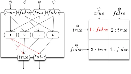
RuleRunner then translates every truth table as a small neural network, creating one input neuron for each possible truth value of the subformula(e), one hidden neuron for each cell in the truth table, and one output neuron for each possible truth value (true, false, undecided). The input-hidden connections implement the compositions of cells in the truth table, and the hidden-output connections map each cell of the truth table onto an output truth value. Figure 4 provides a visual example of the correspondence between extended truth tables and neural networks: the example is simplified to a two-valued disjunction, for the sake of visualisation.

3 4 1 2

...

...

1 :true 2 :true

3 :true 4 :f alse true f alse

f alse true

true f alse

true

true

f alse

f alse

Fig. 4: (Two-valued) disjunction as network and truth table

The weights are computed using theCILP algorithm [8], which is proven to guarantee the following conditions:

C1 the input potential of a hidden neuron h can only exceed its threshold, activatingh, when all the positive antecedents ofhare assigned the truth value true while all the negative antecedents ofhare assigned false. C2 the input potential of an output neuron o can only

exceed its threshold, activating o, when at least one hidden neuron hthat is connected too is activated.

Given an LTL formulaφ, the final output of this encoding phase is a runtime monitor structured as the parsing tree for φ (see Figure 2) where each node corresponds to an LTL operator and contains a neural network (e.g. Figure 4) computing the corresponding extended truth table from (Figure 3). When such a monitor is used to monitor a trace, the current cell’s observations are fed to the neural monitor as input, and the convergence of the feedforward-recurrent propagation in the neural monitor corresponds to the bottom-up labelling process on the formula parsing tree. In [13] we also showed how sparse form representation and parallel computation through GPU can speed up the monitoring process.

IV. LEARNING AS PROPERTY ADAPTATION

A. The Learning Problem

from Business Process Management (where it captures the idea of concept drift) to Multi-agent systems (where autonomous agents can suggest improved solutions to a given task).

As an example, consider a security system built to detect consecutiveloginoperations from the same user with nologout

in between: φ=login_⇒X(!login_∪logout). Now suppose the system detects a number of violations, in a given LAN, that the security manager judges as false positives. For instance, that LAN could be a lab where users log in from different devices, or it could be a trustable section of the network. It is reasonable that the security manager wants to maintain the security system, but also to relax the formal property in order to include logins from the given LAN, and therefore avoid false positives and improve efficiency. Reclassifying a trace means demoting the relation between the observations and the actual output while promoting the relation between observations and expected output: it is, in fact, a supervised learning task. Therefore, wrt. the general framework depicted in Figure 1, the initial property is login ⇒ X(!login∪logout) and the traces are provided by the log of network operations, including logins and logouts. the learning phase modifies the encoded property in order to classify the consecutive logins from the LAN area as non-violations: ideally, the resulting property is

login_⇒X((!login_∨LAN)_∪logout).

The learning process has to be tackled by taking into account both the temporal dimension of the monitoring and the logical structure of the monitor. The intrinsic temporal nature of the monitoring process implies that learning the correct monitoring of a trace corresponds to learning a set of classification instances, one for each cell of the trace. Furthermore, modifying the monitor when analysing a specific cell might alter the behaviour of the monitor on a previously analysed cell, and learning attempts might result in conflicting input-output pairs: we will solve this problem by considering temporary solutions as working hypotheses, and collecting set of said hypotheses before performing batch learning, so that inconsistent options are ignored.

Concerning the kind of formulae that can be learned, our neural monitors present a peculiar structure: on the one hand, we can tweak specific input-output relations within a single operator’s truth table: we are therefore able to learn non-standard logical operators, such as the three-valued correspondent of NAND. This is an interesting feature, whereas several approaches are limited to specific patterns or syntax.

On the other hand, recall that our neural monitors are based

on parsing trees, and the monitoring task correspond to leaves-to-root message passing: in functional terms, learning implies altering the (semantics of the) property encoded in the monitor; in structural terms, it corresponds to modifying the weights of some connections in the neural network. In our system, learning comes with a trade-off between preservation of the initial monitor and learning capability: the balance depends on the degree of freedom we allow during learning. On the one hand, the initial monitor includes a set of properties concerning consistence, truth-table interpretation, sparsity, and so on. On the other hand, if the network is fully connected before the application of the learning algorithm, and every connection in both IH and HO is unconstrained, the learning algorithm can rely on the full network in order to minimise the error function.

In this paper we present an approach based on locally constrained learning, which allows to capture common property modification patterns, such as constraint relaxations and exceptions (exploiting what we called contextual networks). If the exceptions in a set of traces are based on complex temporal patterns that have no common structure with the main property, it seems more reasonable to isolate those traces by standard monitoring and then use a miner to discover independent patterns, rather than trying to merge property and exceptions, when they model syntactically and semantically different patterns.

B. Monitor Structure and Local Learning

In order to describe how to apply learning strategies to our system we need to analyse the structure of its neural monitors. We have mentioned in Section III how the supporting structure for the monitors is the parsing tree of the encoded formula, where each node encodes the operational semantics of a precise operator. These subnetworks are then composed horizontally, as exemplified in Figure 5, in order to form a single-hidden-layer recurrent network (so that suites like Matlab can work with standard topologies), where the global input (resp. hidden, output) layer is the set of all input (resp. hidden, output) neurons of all single subnetworks.

In Figure 5, on the left, is depicted a parsing tree including four (numbered) nodes; the encoding process transforms each node in a single subnetwork. Leaf nodes are encoded as subnetworks that accept observations as inputs (1,3), while the root node (4) computes the final verdict. The arcs of the tree, used to propagate truth values between adjacent nodes,

4

1

2 3

...

... ...

H H H H

I I I

O O O

O

H H H H

I I I

O O O

O

1

2

... ... ...

H H H H

I I I

O O O

O

3

H H H H

I I I

O O O

O

4

... ... ... ...

... ... ...

correspond to the recurrent connections: for instance, since nodes2and3are subnodes of4, the neural network in Figure 5 includes recurrent connections from neurons in the output layers of subnetworks 2and3 to the input layer of subnetwork4.

However, for the learning process, we will consider the subnetworks as organised in the original parsing tree. Note that this double perspective does not require to rearrange the data structure: the tree-based view can be achieved indexing the subnetworks or following the recurrent connections.

It is also worth remarking how these subnetworks are independent: computing A_∨B depends on the truth values of A and B only: for instance, A and B may be complex formulae, and the process of computing their truth values does not affect the_∨ subnetwork; the final verdicts ofAandB are computed independently and propagated from the output layers of A andB to the input layer ofA_∨B.

This structure is ideal for learning small adjustments to the encoded property. For instance, if the encoded property is

XXa∧32(b U c) and the goal is to learn traces generated from XXa_∨32(b U c), the only node in which learning is performed is the one encoding the conjunction. In particular, switching from conjunction to disjunction consists in modifying a few weights in the hidden-output layer in that neural network, as this corresponds to altering the truth values of some cells.

During learning, the weights (and thresholds) are modified according to the adopted learning strategies, like the perceptron adaptation algorithm or the backpropagation algorithm [15]. However, different learning strategies just define the magnitude of each weight update: the sign (increase/decrease) depends solely on the nature of the problem. As an example, consider the neural network (encoding a disjunction) depicted in Figure 4, and suppose that it is used to learn the behaviour of a set of traces. If the traces to be integrated are generated from an agent that performs exclusively φorψ, then the combination of φ

and ψwill yieldf alse: as a result, the learning algorithm will lower the weight of the1_−→trueconnection and increase the weight of the1_−→f alseconnection. After the learning, the hidden neuron 1, when firing, will propagate a signal towards thef alseoutput neuron. The resulting network and truth tables are visualised in Figure 6.

3 4

1 2

...

...

1 :f alse 2 :true

3 :true 4 :f alse true f alse

f alse true

true f alse

true

true

f alse

f alse

Fig. 6: Network and truth table after the learning

Neurons and truth table can be easily re-labelled consulting

a library of stored patterns: in the previous example, the learned operator is an exclusive or (_⊕). Restricting the learning to the hidden-output weight matrix corresponds to training one-layer networks (e.g. a layer of perceptrons), but we do not incur in the theoretical limits of linear separability, as every output neuron implements a disjunction among the connected hidden neurons (representing the cells in the truth table). For instance,

A_⊕B is not linearly separable, buth2_∨h3is: and since the hidden neuronsh2 andh3 correspond, respectively, toA∧!B

and !A_∧B, we obtain (A_⊕B) _≡ ((A_∧!B)_∨(!A_∧B)), which is a valid reformulation of the exclusive disjunction.

C. The Learning Approach

In this subsection we propose a particular learning frame-work - it is worth stressing that the kind of learning we want to implement is aimed at preserving the initially encoded property while including/excluding new patterns: our final goal is to generate adapted monitors that, given a formulaφand a set of labelled traces T, provide the minimal modification of φthat maximises the number of correctly classified traces in T.

For this reason, we restrict the learning to single nodes of the parsing tree, corresponding to precise sets of rules (one operator). The advantages of this approach are several: first of all, we prevent learning from disrupting the hierarchical structure of rules encoded by RuleRunner. Second, this approach preserves the sparsity of the weight matrices in the neural monitor encoding the adapted formula. Third, local learning eases the extraction process, allowing to compute a symbolic description of the learned formula(e). The disadvantage of this approach is that we are constraining the learning capabilities of the system, limiting the search space to a syntactical neighbourhood of the initial formula.

The learning approach we propose is composed by two phases: first, local training sets are collected, and subsequently a learning strategy is applied on each training set.

The starting point for learning is a monitor encoding an initial formulaφand a set of labelled traces. The labels of the traces represent the desired monitoring verdict, which might not correspond to the actual output of the monitor encoding

φ. There are two possible scenarios for the collection of these traces:

• A third-party system is observed and all of its trajec-tories are used as positive cases; the traces are then verified against the initial monitor forφ.

• The initial monitor forφlabels all traces, and a domain expert modifies the verdict for the cases that he wants the monitor to include/exclude.

... ...

...

...

...

verdict

observation observation

... ...

...

...

...

label

(a) (b)

Fig. 7: Forward/backward propagation

Once the actual output (verdict) is computed, it can be compared with the desired one, provided by the trace label. Since we are interested in modifying the highlighted node only, we need to infer the desired output for that specific node, and we compute it by a backwards propagation from the root node to the highlighted one (Figure 7(b)). So the monitor is used to propagate (forward) the actual global output and, if it differs from the expected label, to propagate (backward) the local expected output for the highlighted node. Note that the backward propagation of the expected output corresponds to abduction.

At this point, we do have the couple of actual input

and desired output for the selected node: the former was computed in the monitoring step, while the latter was obtained by backwards propagation, starting from the desired label. We store this couple of values, force the expected output in the selected node, and move to the next cell. We do so for the following reasons:

• We know that by forcing the output of the selected node to match the desired one, the remaining forward propagation will produce the expected label, thus allowing -if necessary - to proceed with the monitoring. Thus we use the input-output behaviour as aworking hypothesis

in order to proceed with the monitoring/learning.

• We store the actual input/desired output as part of the training set for the selected node. By doing so, we postpone all actual learning to a subsequent phase, where it can be applied to a whole training set (batch approach).

...

_

... ...

...

...

Input Output ... ... Input Output Input Output ... ... Input Output

Input Output ... ... Input Output Input Output

... ... Input Output Input Output ... ... Input Output

Fig. 8: Collecting local training sets

At the end of this phase, for each node in the initial monitor a training set has been built (Figure 8). Note that we simply defined each element as an input-output pair, but in fact input and output are activation patterns on the input/output layer of the selected node. In the second phase, learning strategies can be exploited to make each subnetwork match the input-output behaviour represented by the corresponding local training set; all these training tasks are independent and can be run in parallel.

At the end of this phase the best performing subtest can be selected and the corresponding operator modified accordingly; this compose a single learning step, as the resulting network can undergo another learning phase in order to modify another operator and further improve the general accuracy.

D. Contextual Subnetworks

So far we focused on learning tasks where the desired behaviour was an alteration of the encoded property, commonly by means of a relaxation of some connective. However, it may be the case that the desired behaviour depends on additional observations that do not belong to the initial formula. This happens, for instance, withexceptions, where a specific case can be isolated and exempted from a general rule.

A neural monitorN Nφ, as it is, is not suitable for learning behaviours including new observations, as everything which is not included in the original property is filtered. This is reasonable for the ‘pure monitoring’ phase, as the size of observations provided by the observed system may be arbitrarily big wrt. the few observations to be monitored. However, when adapting the monitor in order to learn to re-classify traces, taking new observations into account may be necessary. A simple example for this particular issue was provided with the example concerning the security domain: the initial property did not include details about the LAN, so that information was initially ignored by the monitor.

In structural terms, the neural monitor may lack the actual input neurons necessary to be aware of some observations. In order to overcome this limitation, the topology of the neural network has to be modified in order to detect the desired observations and be able, through learning, to connect them with the rest of the network, so that the occurrence of the new observation influence the overall semantics of the monitor. We call contextual subnetwork fora(CSa_{) the subnetwork added} to the initial neural monitor in order to take into account the occurrence of an observation a.

As a minimum requirement,CSa_{must include an input} neu-ron labelleda, so that the activation of the neuron corresponds to the occurrence ofa in the current cell. However, this is not sufficient in our convergence-based approach, as the monitoring of a subformula requires several feed-forward propagations in the neural monitor, and ahas to be ‘remembered’ throughout this phase; we therefore also introduce an hidden and output neuron.

The minimal CSa _{for an observationa is therefore} visu-alised in red in Figure 9, and it corresponds to the simple logic program:

R.. R.. x

F S ..

R.. R.. x

F S ..

a

a

N N f or N N f or

Fig. 9: Minimal contextual subnetwork fora

However, as we have observed in the previous subsections, it is often the case that the occurrence of an observation and its impact on the desired final verdict belong to two different cells; in order to satisfy this need of through-time persistence, we propose a second type of contextual subnetwork which remem-bers whether a given observation owas always/sometimes true in the past. This extended contextual subnetwork, highlighted in Figure 10, corresponds to the following logic program:

a _⇒a _| a _⇒3a _| 3a _⇒3a _| (2a _∧ a)_⇒2a

The first clause corresponds to the minimal contextual network, and it is used to link the occurrence ofawith the output pattern of the neural monitor. The second and third clauses model the existential occurrence of a: if a is observed, then 3a holds from that cell; if 3aholds, it is maintained in the future cells. The fourth clause model the universal existence ofa: as long as ais observed,2aholds.

R.. R.. x

F S ..

R.. R.. x

F S ..

a

a <>a

(or)

<>a []a

(and)

[]a

N N f or N N f or

Fig. 10: Extended contextual subnetwork fora

Specific contextual networks can be built in order to meet specific needs; for instance, delay-units can be exploited to build contextual networks that take into account exceptions that occurred in the previous cell.

Contextual networks provide additional inputs for the neural monitor, but are initially disconnected from the neural monitor and have no impact on the monitoring process; it is necessary to apply a learning strategy to connect the main neural monitor and the built contextual networks, so that the occurrence of exceptions impacts on the monitoring verdict. The general approach presented in the previous subsection can also be used to learn exceptions, e.g. unpredicted patterns that involve atoms (observations) not included in the original formula. We use precisely the same set of algorithms, with one single difference: the focus node is not selected on the tree of the original monitor, but added ex novo, connecting the neural monitor with a contextual network.

The approach is sketched in Figure 11: in any edge from a node A to a node B, a new dummy node, called Graf t

in figure, can be inserted. Initially the node computes a left-projection function, so that it simply propagates the output of theB node as input to theAnode. A contextual network is added as right subnode of theGraf t. The contextual network can store arbitrary information about a given atom, or set of atoms, not previously included in the initial formula (which the

main tree is monitoring). In the simplest case, the contextual subnetwork for a given observationxsimply detects whetherx

holds in the current trace. Using theGraf tnode asfocusnode in the learning process allows the monitor totake into account

the information computed and stored in the contextual node and to let it influence the verdict of the adapted monitor, if this improves the monitoring accuracy. The richness of symbolical information about the evaluation status of all subformulae of the currently monitored property allows us to decide where to graft the contextual node with surgical precision, measuring its impact on different nodes in independent tests.

A

B

...

... ... ...

A

B

...

... ...

... Graft

Context

Fig. 11: Grafting a contextual subnetwork to a monitoring tree

E. Example

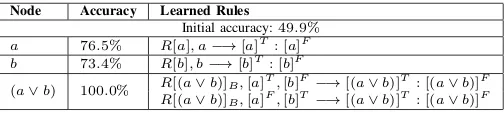
In this section we present two examples of property adaptation, measuring the accuracy of the adapted monitor and providing a qualitative analysis of the learned rules. We will use the notation Body _−→ Head1 : Head2 to indicate when the learning process modified theBody−→Head1 rule into Body _−→Head2. More practically, providing the pair

{Body, Head2}to the learning algorithm, the weight of the connection from the hidden neuron representing the current rule (let it be h) to the output neuron labelled Head1 was reduced, while the weight of the connection from h and the output neuron labelled Head2 was augmented.

The first example is the adaptation of a disjunction into a conjunction. The initial accuracy is roughly 50%. For this simple example, it is easy to see why: the cases with bothaand

bor neitheranorbare classified (respectively, asSU CCESS

and F AILU RE) by M(a∨b) in a consistent way with the expected label specified by(a∧b). The traces where exclusively

aor boccur are classified asSU CCESS against an expected

F AILU RE label.

Node Accuracy Learned Rules

Initial accuracy:49.9% a 76.5% R[a], a−→[a]T : [a]F b 73.4% R[b], b−→[b]T : [b]F

(a∨b) 100.0% R[(a∨b)]B,[a]T,[b]F −→[(a∨b)]T : [(a∨b)]F R[(a∨b)]B,[a]F,[b]T−→[(a∨b)]T : [(a∨b)]F

TABLE II: Froma_∨b toa_∧b

The nodesaandbprovide baseline-level accuracies (76.5%

the two learned rules correspond, by the way, to the different truth values between the binary truth tables of conjunction and disjunction.

As second example, we describe the adaptation of(aU b)to 3b (Table III): in this case we haven’t modified one operator, but used a different syntax to express a similar property (recall that (_>U b)_≡3b).

Node Accuracy Learned Rules

Initial accuracy:49.4% a 100.0% R[a],!a−→[a]F _{: [a]}T b 100.0% R[b],!b−→[b]F : [b]?

(aU b) 100.0%

R[(aU b)]A,[a]F,[b]F−→[(aU b)]F : [(aU b)]?_AP R[(aU b)]R,[b]F]−→[(aU b)]F : [(aU b)]?BP R[(aU b)]B,[a]F,[b]T−→[(aU b)]F : [(aU b)]T R[(aU b)]L,[a]F −→[(aU b)]F : [(aU b)]T R[(aU b)]B,[a]F,[b]F−→[(aU b)]F : [(aU b)]?_LP

TABLE III: From(aU b)to3b

In the (aU b)node, the learning algorithm adapted a set of rules (recall how rich the evaluation tables forU are). The first, second and fifth rules take into account situations where

b is false, forcing the result from false to undecided: since in fact the traces are labelled according to the formula 3b, a failure of bjust requires the whole monitoring to proceed. The second rule forces the monitor to yield a true result when b is observed, ignoring the fact that afailed: this mirrors the fact that in3b ais irrelevant. The third rule, similarly, expresses the fact that when only the monitoring of ais pending (and this means thatb already succeeded), the monitoring of theU

formula terminates with a positive verdict.

In thebnode the learning process produced a single updated rule: R[b],!b −→[b]F _{: [b]}?_{. This may look weird, as it is a} mere observation being assigned an undecided truth value. In fact, as long as b is not observed, [b]? _{is inferred, and this} causes the super-formula(aU b)to iterate on the following cell. If ais not observed, theuntilsimply switches from theA to theB sub-states (see [13]): the system has just found another way to ignorea. If eventuallybis observed,[b]T _{and[(aU b)]}T are inferred, causing the monitoring of the trace to produce a

SU CCESS verdict. Ifbis never observed, the(aU b)formula reaches the end of the trace, where theEN D rules force the undecided status of the untilto false.

In theanode, the system learned the adaptation that requires less explanations both in terms of syntax and semantics: a

becomes a constant function returning true, therefore we go from (aU b)to(>U b)≡3b.

V. CONCLUSIONS ANDFUTUREWORK

In this paper, we extend our neural monitoring system RuleRunner, equipping the framework with a learning module in order to allow a monitor to adapt to new models or include unexpected exceptions.

We suggested an original light-weight learning approach that restricts the search space to the syntactical neighbourhood of the monitored temporal formula: this allows to implement adaptation as a set of targeted, independent learning tasks in isolated subnetworks. Despite the neural encoding, we always maintain the symbolic interpretation of our monitor, even after learning, thus allowing for instantaneous symbolic extraction of

the adapted formula(e). The best performing adapted monitor can be therefore extracted as a new temporal property and used for another iteration.

The learning approach we proposed is limited to a syntac-tical neighbourhood of the encoded specification. A reasonable direction for future work would be a wider comparison of learning strategies, in terms of accuracy, performance, and quality of the extracted pattern. Once again, this depends from the desired application: if a symbolic representation of the learned patterns is required, training one layer proved to be a valid choice; on the other hand, if the user wants to use the adapted monitor as a benchmark, less structure-preserving learning strategies would make a valid option, as in that case there would be no symbolic extraction.

REFERENCES

[1] H. Barringer, D. E. Rydeheard, and K. Havelund. Rule systems for run-time monitoring: from eagle to ruler. J. Log. Comput., 20(3):675–706, 2010.

[2] A. Bauer, M. Leucker, and C. Schallhart. Monitoring of real-time properties. Lecture Notes in Computer Science, pages 260–272, 2006. [3] R. V. Borges, A. S. d’Avila Garcez, and L. C. Lamb. Learning and representing temporal knowledge in recurrent networks. IEEE Transactions on Neural Networks, 22(12):2409–2421, 2011.

[4] A. Cimatti, E. Clarke, F. Giunchiglia, and M. Roveri. Nusmv: a new symbolic model checker. International Journal on Software Tools for Technology Transfer, 2000.

[5] A. S. d’Avila Garcez and G. Zaverucha. The connectionist inductive learning and logic programming system. Appl. Intell., 11(1):59–77, 1999.

[6] D. Drusinsky. The temporal rover and the atg rover. InSPIN, volume 1885 ofLecture Notes in Computer Science, pages 323–330. Springer, 2000.

[7] B. Finkbeiner and H. Sipma. Checking finite traces using alternating automata. Electr. Notes Theor. Comput. Sci., 55(2):147–163, 2001. [8] A. S. d. Garcez, G. Zaverucha, and L. A. V. de Carvalho. Logical

inference and inductive learning in artificial neural networks.Knowledge Representation in Neural networks, pages 33–46, 1997.

[9] D. Giannakopoulou and K. Havelund. Automata-based verification of temporal properties on running programs. InProceedings of the 16th IEEE International Conference on Automated Software Engineering, ASE ’01, pages 412–. IEEE Computer Society, 2001.

[10] K. Havelund and G. Rosu. Monitoring programs using rewriting. In

Proceedings of the 16th IEEE International Conference on Automated Software Engineering, ASE ’01, pages 135–. IEEE Computer Society, 2001.

[11] S. Haykin. Neural Networks: A Comprehensive Foundation. Prentice Hall, 1999.

[12] M. Leucker and C. Schallhart. A brief account of runtime verification.

J. Log. Algebr. Program., 78(5):293–303, 2009.

[13] A. Perotti, A. S. d’Avila Garcez, and G. Boella. Neural networks for runtime verification. In2014 International Joint Conference on Neural Networks, IJCNN 2014, Beijing, China, July 6-11, 2014, pages 2637–2644. IEEE, 2014.

[14] A. Pnueli. The temporal logic of programs. InProceedings of the 18th Annual Symposium on Foundations of Computer Science, pages 46–57, Washington, DC, USA, 1977. IEEE Computer Society.

[15] F. Rosenblatt. Principles of Neurodynamics. Spartan, New York, 1962. [16] G. Rosu and K. Havelund. Rewriting-based techniques for runtime

verification. Autom. Softw. Eng., 12(2):151–197, 2005.

[17] H. T. Siegelmann, B. G. Horne, and C. L. Giles. Computational capabilities of recurrent narx neural networks. IEEE Transactions on Systems, Man, and Cybernetics, Part B, 27(2):208–215, 1997. [18] L. Zhao, T. Tang, J. Wu, and T. Xu. Runtime verification with