City, University of London Institutional Repository
Citation:
Sun, H., Xu, H., Meskarian, R. and Wang, Y. (2013). Exact penalization, level
function method, and modified cutting-plane method for stochastic programs with second
order stochastic dominance constraints. SIAM Journal on Optimization (SIOPT), 23(1), pp.
602-631. doi: 10.1137/110850815
This is the unspecified version of the paper.
This version of the publication may differ from the final published
version.
Permanent repository link:
http://openaccess.city.ac.uk/2414/
Link to published version:
http://dx.doi.org/10.1137/110850815
Copyright and reuse: City Research Online aims to make research
outputs of City, University of London available to a wider audience.
Copyright and Moral Rights remain with the author(s) and/or copyright
holders. URLs from City Research Online may be freely distributed and
linked to.
City Research Online:
http://openaccess.city.ac.uk/
[email protected]
MODIFIED CUTTING-PLANE METHOD FOR STOCHASTIC PROGRAMS WITH SECOND ORDER STOCHASTIC DOMINANCE
CONSTRAINTS
HAILIN SUN∗, HUIFU XU†, RUDABEH MESKARIAN‡, AND YONG WANG§
Abstract. Level function methods and cutting plane methods have been recently proposed to solve stochastic programs with stochastic second order dominance (SSD) constraints. A level function method requires an exact penalization setup because it can only be applied to the objective function, not the constraints. Slater constraint qualification (SCQ) is often needed for deriving exact penalization. It is well known that SSD usually does not satisfy SCQ and various relaxation schemes have been proposed so that the relaxed problem satisfies the SCQ. In this paper, we show that under some moderate conditions the desired constraint qualification can be guaranteed through some appropriate reformulation of the constraints rather than relaxation. Exact penalization schemes based onL1-norm andL∞-norm are subsequently derived through Robinson’s error bound on convex system and Clarke’s exact penalty function theorem. Moreover, we propose a modified cutting plane method which constructs a cutting plane through the maximum of the reformulated constraint functions. In comparison with the existing cutting plane methods, it is numerically more efficient because only a single cutting plane is constructed and added at each iteration. We have carried out a number of numerical experiments and the results show that our methods display better performances particularly in the case when the underlying functions are nonlinear w.r.t. decision variables.
Key words. Slater constraint qualification, exact penalization, modified cutting-plane method, level function method
AMS subject classifications. 90-08, 90C15, 90C30, 90C90
1. Introduction. Stochastic dominance is a fundamental concept in decision theory and economics. A random outcomea(ω) is said to dominate another random outcomeb(ω) in the second order, written asa(ω)≽2b(ω), ifE[v(a(ω))]≥E[v(b(ω))] for every concave nondecreasing functionv(·), for which the expected values are finite, see monograph [17] for the recent discussions of the concept.
In their pioneering work [4], Dentcheva and Ruszczy´nski introduced a stochastic programming model with second order stochastic dominance constraints :
min
x E[F(x, ξ(ω))]
s.t. G(x, ξ(ω))≽2Y(ξ(ω)), x∈ X,
(1.1)
where X is a closed convex subset of IRn, ξ: Ω→Ξ is a vector of random variables defined on probability space (Ω,F, P) with support set Ξ⊂IRq,F : IRn×Ξ→IR is convex continuous function w.r.t. x,G: IRn×Ξ→IR is concave continuous function w.r.t. xandE[·] denotes the expected value with respect to the distribution ofξ(ω).
∗Department of Mathematics, Harbin Institute of Technology, Harbin, 150001, China ([email protected]).
†School of Engineering and Mathematical Sciences, City University London, London, EC1V 0HB, London, UK; School of Maritime and Transportation, Ningbo University, China. ([email protected]).
‡School of Mathematics, University of Southampton, Southampton, SO17 1BJ, UK ([email protected]).
§Department of Mathematics, Harbin Institute of Technology, Harbin, 150001, China ([email protected]).
Here we make a blanket assumption that the expected value of the random function is well defined.
A simple economic interpretation of the model can be given as follows. Let G(x, ξ(ω)) be a profit function which depends on decision vector x and a random variable ξ(ω), let F =−G and Y(ξ(ω)) be a benchmark profit. Then (1.1) can be viewed as an expected profit maximization problem subject to the constraint that the profit dominates the benchmark profit in second order.
LetF1(X;η) denote cumulative distribution function of random variableX, that is,
F1(X;η) :=P(X ≤η),
and
F2(G(x, ξ(ω));η) :=
∫ η
−∞
F1(G(x, ξ(ω));t)dt.
G(x, ξ(ω)) is said to dominate Y(ξ(ω)) in first order, denoted by G(x, ξ(ω)) ≽1 Y(ξ(ω)), if for allη∈IR,
F1(G(x, ξ(ω));η)≤F1(Y(ξ(ω));η).
G(x, ξ(ω)) is said to dominate Y(ξ(ω)) in second order, denoted by G(x, ξ(ω)) ≽2 Y(ξ(ω)), if
F2(G(x, ξ(ω));η)≤F2(Y(ξ(ω));η),∀η∈IR. (1.2)
It is easy to observe that first order stochastic dominance implies second order s-tochastic dominance. It is well known that second order dominance constraint in (1.1) can be reformulated as
E[(η−G(x, ξ(ω)))+]≤E[(η−Y(ξ(ω)))+], ∀η∈IR, (1.3)
where (x)+ = max(0, x); see [6]. Ogryczak and Ruszczy´nski [18] investigated the relationship between stochastic second order dominance and mean-risk models. In a more recent development [5, Theorem 3.1], the second order dominance is shown to be equivalent to a continuum of conditional value at risk constraints: one for each probability level. Using the reformulation of the second order dominance constraints, Dentcheva and Ruszczy´nski [6] reformulated (1.1) as:
min
x E[F(x, ξ(ω))]
s.t. E[(η−G(x, ξ(ω)))+]≤E[(η−Y(ξ(ω)))+], ∀η∈IR, x∈ X.
(1.4)
To ease notation, we will useξto denote the random vectorξ(ω) and a deterministic vector, depending on the context. It is well known that (1.4) does not satisfy the well known Slater constraint qualification, a condition that is often needed for deriving first order optimality conditions of the problem and developing a numerically stable method for solving the problem. Subsequently, a so-called relaxed form of (1.4) is proposed:
min
x E[F(x, ξ)]
s.t. E[(η−G(x, ξ))+]≤E[(η−Y(ξ))+], ∀η∈[a, b], x∈ X,
where [a, b] is a closed interval in IR. Over the past few years, Dentcheva and Ruszczy´nski have developed comprehensive theory of optimality and duality for (1.5), see [4, 5, 6].
Unfortunately, problem (1.5) is difficult to solve since it is a stochastic semi-infinite nonsmooth programming problem. In the case whenG(x, ξ) and F(x, ξ) are linear w.r.t. x and ξ has finitely many scenarios, Dentcheva and Ruszczy´nski [5] reformulated problem (1.5) as a linear programming (LP) problem by introducing new variables which represent positive parts in each constraint of problem (1.5). The reformulation effectively tackles the nonsmoothness in the second order constraints and the approach can easily be used to the case whenGand F are nonlinear. This reformulation, however, introduces many new variables particularly when the random variableξhas many distributional scenarios. Apparently this does not have significant impact on numerical implementation as the existing solvers for LP are very powerful (can deal with millions of variables). However, the impact will be much more signifi-cant whenF andGare nonlinear and this is indeed one of the key issues this paper is to address.
Rudolf and Ruszczy´nski [22] and F´abi´an et al [8] proposed cutting-plane methods for solving a stochastic program with second order stochastic dominance constraints. A crucial element of the method in [8] is based on an observation that whenF and G are linear w.r.t. x and probability space Ω is finite, the constraint function in the second order dominance constraint is the convex envelope of a finitely many lin-ear functions, which is called cutting-plane representation and observed by Haneveld and van der Vlerk in [11]. Subsequently, an iterative scheme which exploits the fun-damental idea of classical cutting-plane method is proposed where at each iterate “cutting-plane” constraints are constructed and added. This also effectively tackles the nonsmoothness issue caused by the plus function. While the method displays strong numerical performance, it relies on discreteness of the probability space as well as the linearity ofF and G. Hu, de-Mello and Mehrotra [10] and Homem-de-Mello and Mehrotra [9] also proposed a cut generation algorithm for solving a sample average approximation (SAA) problem of stochastic program with multivari-ate stochastic dominance constraints. Different from the cutting plane method in [22] and [8], they reformulated every subproblem as linear programming problem by introducing some new variables whenF andGare linear.
In this paper we consider problem (1.4) with a focus on the case whenξ has a discrete distribution, that is,
min
x N
∑
i=1
piF(x, ξi)
s.t.
N
∑
i=1
pi(η−G(x, ξi))+≤
N
∑
i=1
pi(η−Y(ξi))+, η∈IR,
x∈ X.
(1.6)
Here the random variable ξ has a finite distribution, that is, P(ξ = ξi) = pi, for
i = 1,· · · , N. When pi = N1, problem (1.6) can be viewed as a sample average
approximation of problem (1.4). We investigate the Slater constraint qualification of the problem and its reformulation, exact penalization schemes and numerical methods. Specifically, we make the following contributions.
error bound [19]. The latter requires SCQ. Unfortunately, problem (1.6) or its reformulation (2.5) does not satisfy the constraint qualification (see dis-cussions by Dentcheva and Ruszczy´nski at pages 558-559 in [4]). Here we propose an alternative way to reformulate the constraints of problem (2.5). We then demonstrate that the newly reformulated problem (see (2.7)) satisfies the SCQ under some moderate conditions (see Theorem 2.1). Two exact pe-nalization schemes based onL1-norm andL∞-norm are subsequently derived and are shown that they are exact penalization of problem (2.5) although the latter does not satisfy SCQ (see Theorems 3.1 and 3.2). Note that Liu and Xu [14] proposed an exact penalization scheme withL∞-norm for the relaxed problem (1.5). A crucial condition is the SCQ of problem (1.5) which relies on therelaxationbecause the original problem (1.4) may not satisfy the SCQ. Our penalization schemes in this paper differ from Liu and Xu’s in that they are proposed for the original problem rather than for the relaxed problem, which means that they are established without the SCQ of the original prob-lem. This makes the penalization scheme more appealing given the fact that the original problem usually does not satisfy the SCQ particularly in the case whenξ satisfies discontinuous distribution. Based on the exact penalization formulations, we apply a well known level function method in nonsmooth optimization [13, 25] to the penalized problems. An obvious advantage of this approach is that we can effectively deal with excessive number of con-straints, nonsmoothness in the constraints and nonlinearity of the underlying functions.
• We also propose a modified cutting-plane method to solve the problem. The cutting-plane method differs from those in the literature [22] in that it ap-plies to the maximum of the constraint functions rather than each constraint function. This saves considerable computation time because at each itera-tion, our cutting-plane method requires to add a couple of linear constraints whereas the cutting-plane method in [22] requires to addN constraints (N is the cardinality of the support set Ξ). The approach also differs from that in [9, 10] because our modified cutting-plane method uses the cutting-plane rep-resentation proposed in [11]. The idea of applying the cutting-plane method to the maximum of the constraint functions is similar to the idea in algorithm proposed by F´abi´an, Mitra and Roman, see the algorithm at page 48 in [8]. Note that F´abi´an, Mitra and Roman’s algorithm is applied to linear models while Algorithm 4.1 is applicable to nonlinear case. Therefore we may regard our algorithm as an extension of theirs.
• We have carried out extensive numerical tests on our proposed methods in comparison with the cutting plane method in [8]. The numerical results show that our proposed methods are more efficient. Specifically, we have discovered that level function method based on exact penalization scheme with L∞-norm is most efficient in terms of computation time; the modified cutting-plane method (Algorithm 4.1) performs also efficiently.
advan-tage of doing this is to apply stochastic approximation methods (e.g. [7]) other than SAA.
The rest of the paper is organized as follows. In section 2, we discuss the SCQ of problem (1.6) and its reformulation. In section 3, we propose two exact penalization schemes for problem (2.5) and apply a level function method to solve them. In section 4, a modified cutting-plane method has been proposed for solving the problem and finally in section 5, we report some numerical test results.
Throughout this paper, we use the following notation. xTy denotes the scalar
product of two vectorsxandy,∥ · ∥,∥ · ∥1and∥ · ∥∞denote the Euclidean norm,L1 -norm andL∞-norm of a vector and a compact set of vectors respectively. We also use ∥ · ∥to denote the infinity norm of a continuous function space and its induced norm of a linear operator. d(x,D) := infx′∈D∥x−x′∥, d1(x,D) := infx′∈D∥x−x′∥1 and d∞(x,D) := infx′∈D∥x−x′∥∞denote the distance from pointxto setDin Euclidean norm, L1-norm and L∞-norm respectively. For a real valued-function h(x), we use ∇h(x) to denote the gradient ofhatx.
2. Slater constraint qualification. In the literature of stochastic programs with second order dominance constraints, SCQ has been used as a key condition for deriving optimality conditions and exact penalization, see for instances [4, 14].
Recall that problem (1.6) is said to satisfies the SCQ if there existsx0∈ X such that
N
∑
i=1
pi(η−G(x0, ξi))+−
N
∑
i=1
pi(η−Y(ξi))+<0, η∈IR. (2.1)
Unfortunately, this kind of constraint qualification is not satisfied. To see this, let
Y(Ξ) :={Y(ξi) :i= 1,· · ·, N}
and
y:= min{Y(ξ1),· · ·, Y(ξN)}. (2.2)
For any η≤y, it is easy to verify that E[(η−Y(ξ))+] = 0. For thoseη, the feasible constraint of problem (1.5) reduces to
E[(η−G(x, ξ))+]−E[(η−Y(ξ))+] = 0
because the term at the left hand side of the equation is non-negative. This means that there does not exist a feasible pointx0∈ X such that (2.1) holds.
Dentcheva and Ruszczy´nski [4] observed this issue and tackled it by considering a relaxed problem (1.5) which effectively restrictsη to take value from a specified [a, b]. In other words, the feasible region of the original problem (1.6) is enlarged. In this context, their relaxation scheme can be written as follows:
min
x N
∑
i=1
piF(x, ξi)
s.t.
N
∑
i=1
pi(η−G(x, ξi))+≤
N
∑
i=1
pi(η−Y(ξi))+, η∈[a, b],
x∈ X.
Under some circumstance, it is possible to choose a proper valueasuch that problem (2.3) satisfies the SCQ. For instance, if there exists a pointx0∈ X such that
G(x0, ξ)≽1Y(ξ)
and for everyξ∈Ξ,G(x0, ξ)> y, thenx0 is a feasible point of problem (2.3) and
∫ η
−∞
F1(G(x0, ξ);t)dt <
∫ η
−∞
F1(Y(ξ);t)dt
for all η > y. In such a case, it is easy to verify that the SCQ holds for anya > y. Note that problem (2.3) is a relaxed problem of (1.6) which depends on [a, b] and when [a, b] containsY(Ξ), the SCQ fails.
Hu, Homem-de-Mello and Mehrotra [10] proposed an alternative approach to deal with the SCQ issue by consideringϵ-feasible solutions:
min
x E[F(x, ξ(ω))]
s.t. E[(η−G(x, ξ(ω)))+]≤E[(η−Y(ξ(ω)))+] +ϵ, ∀η∈IR, x∈ X.
(2.4)
where ϵ is a small positive number. It is easy to observe that the relaxed problem satisfies the SCQ for any positive ϵ as long as the original problem is feasible. A theoretical issue to be addressed in the aforementioned relaxation schemes is to show that the feasible solution set of the relaxed problem approximates the feasible solution set of the original problem, which often in turn requires the original problem to satisfy certain regularity conditions (to ensure lower semicontinuity of the feasible solution set of the relaxed problems).
In this section, we propose an alternative way to address the issue of SCQ of problem (1.6) without relaxation. To this end, let us use [4, Proposition 3.2] to reformulate problem (1.6) as follows:
min
x N
∑
i=1
piF(x, ξi)
s.t.
N
∑
i=1
pi(Yj−G(x, ξi))+≤γj, j= 1, . . . , N,
x∈ X,
(2.5)
where Yj := Y(ξj), γj :=
∑N
i=1pi(Yj −Yi)+. Like the original problem (1.6), the reformulated problem (2.5) does not satisfy SCQ.
We consider the power set of {1, . . . , N}, that is, a collection of all subsets of {1, . . . , N}including empty set and itself. For the simplicity of notation, letN denote the power set excluding the empty set and forj= 1, . . . , N,
ψj(x) := max
J ∈N
∑
i∈J
pi(Yj−G(x, ξi))−γj. (2.6)
Consider problem
min
x
∑N
i=1piF(x, ξi)
s.t. ψj(x)≤0,forj= 1, . . . , N,
x∈ X.
Note that (2.7) is similar to the cutting plane representation in [8, 22]. The key difference is that hereJ is restricted to take a nonempty subset of{1, . . . , N}, which allows maxJ ∈N∑i∈Jpi(Yj−G(x, ξi)) to take a negative value (otherwise the term
is nonnegative as∑i∈Jpi(Yj−G(x, ξi)) = 0 forJ =∅). This paves the way for (2.7)
to satisfy the SCQ in later discussions. In what follows, we will show that problem (2.7) is equivalent to problem (2.5) but, under some circumstance, the former satisfies the SCQ.
Lemma 2.1. Forj= 1,· · ·, N, let
φj(x) := max
J ∈N
∑
i∈J
pi(Yj−G(x, ξi)).
Then
N
∑
i=1
pi(Yj−G(x, ξi))+= max{φj(x),0}. (2.8)
Proof. We prove the claim by going through two cases: 1. φj(x)≤0; 2. φj(x)>0.
Case 1. Since φj(x) ≤ 0, then max{φj(x),0} = 0 and Yj −G(x, ξi) ≤ 0 for
j∈ {1, . . . , N}. The latter implies
N
∑
i=1
pi(Yj−G(x, ξi))+= 0
and hence (2.8).
Case 2. Since φj(x)> 0, then there exists a nonempty subsetJ ⊆ {1, . . . , N}
such that
φj(x) =
∑
i∈J
pi(Yj−G(x, ξi))>0.
It suffices to show that
∑
i∈J
pi(Yj−G(x, ξi)) = N
∑
i=1
pi(Yj−G(x, ξi))+
or equivalentlyJ contains every indexiwithYj−G(x, ξi)>0. Indeed, ifJ does not
include such an index, then adding it toJ would increase the quantity∑i∈Jpi(Yj−
G(x, ξi)) and this contradicts the fact thatφ
j(x) is the maximum. Likewise,J does
not contain an indexiwithYj−G(x, ξi)<0, because, otherwise, removing the index
will also increase the quantity∑i∈J pi(Yj−G(x, ξi)). This completes the proof.
We are now ready to state the main result in this section.
Theorem 2.1. Let G(x, ξ) and Y(ξ) be defined as in problem (1.6) and ψj be
defined as in (2.6). Then
(i) G(x, ξ)≽2Y(ξ) if and only if
ψj(x)≤0, ∀j = 1, . . . , N; (2.9)
(ii) problems (2.5) and (2.7) are equivalent;
(iii) if there exists a feasible pointx0such thatG(x0, ξ)≽1Y(ξ)andG(x0, ξ)> y
Proof. Part (i). By [4, Proposition 3.2], G(x, ξ)≽2Y(ξ) if and only if
N
∑
i=1
pi(Yj−G(x, ξi))+≤γj, j= 1, . . . , N, (2.10)
or equivalently forj= 1,· · · , N,
max
{N ∑
i=1
pi(Yj−G(x, ξi))+−γj,0
}
= 0.
By (2.8)
max
{ N ∑
i=1
pi(Yj−G(x, ξi))+−γj,0
}
= max{max{φj(x),0} −γj,0}.
Note that for any numbera∈IR andr >0, it is easy to verify that
max{max{a,0} −r,0}= max{a−r,0}. (2.11)
Using (2.11), we have that
max{max{φj(x),0} −γj,0}= max{φj(x)−γj,0}= max{ψj(x),0}.
The last equality is due to the definition of ψj. The discussion above demonstrates
that (2.10) is equivalent to (2.9) and hence the conclusion.
Part (ii) follows straightforwardly from Part (i) in that the feasible set of the two problems coincide, i.e.,
{
x∈ X :
N
∑
i=1
pi(Yj−G(x, ξi))+−γj≤0
}
={x∈ X :ψj(x)≤0}.
Part (iii). Let γy :=
∑N
i=1pi(y−Y(ξi))+, where y is defined in (2.2). By the definition of y, the right hand side equals to 0. Therefore γy = 0. Likewise, the
assumptionG(x0, ξ)> yforξ∈Ξ implies
∑
i∈J
pi(y−G(x0, ξi))<0
for every nonempty index setJ ⊆ {1, . . . , N}. This shows
max J ∈N
∑
i∈J
pi(y−G(x0, ξi))−γy <0. (2.12)
Assume without loss of generality that the N elements in set Y(Ξ) satisfies the fol-lowing order
Y1≤Y2≤ · · · ≤YN.
By the definition ofψj(x) (see (2.9), inequality (2.12) means that
ψ1(x0) = max J ∈N
∑
i∈J
pi(Y1−G(x0, ξi))−
N
∑
i=1
In what follows, we showψj(x0)<0, for j= 2,· · ·, N. By definition
ψj(x0) = max
J ∈N
∑
i∈J
pi(Yj−G(x0, ξi))− N
∑
i=1
pi(Yj−Y(ξi))+
≤max
{
max J ∈N
∑
i∈J
pi(Yj−G(x0, ξi)),0
}
− N
∑
i=1
pi(Yj−Y(ξi))+
=
N
∑
i=1
pi((Yj−G(x0, ξi))+−(Yj−Y(ξi))+)
=
∫ Yj
−∞
(
F1(G(x0, ξ), t)−F1(Y(ξ), t))dt. (2.13)
The second last equality follows from Lemma 2.1 and the last equality is due to the equivalent representation of second order dominance between (1.2) and (1.3).
Assume without loss of generality thatY2> Y1 (otherwiseψ2(x0) =ψ1(x0)<0). Let ¯η∈(Y1,min{min
ξ∈ΞG(x0, ξ), Y2}). Note that, by assumption,Y1<min{minξ∈ΞG(x0, ξ), Y2}, ¯
η exists. Then
∫ Yj
−∞
F1(G(x, ξ), t)−F1(Y(ξ), t)dt =
∫ η¯
−∞
F1(G(x, ξ), t)−F1(Y(ξ), t)dt
+
∫ Yj
¯
η
F1(G(x, ξ), t)−F1(Y(ξ), t)dt.
Note that
∫ η¯
−∞
F1(G(x, ξ), t)−F1(Y(ξ), t)dt= 0−p1(¯η−Y1)<0
wherep1 is the probability thatY(ξ) takes valueY1. On the other hand,G(x0, ξ)≽1 Y(ξ) implies
∫ Yj
¯
η
(F1(G(x0, ξ), t)−F1(Y(ξ), t))dt≤0.
This shows
∫ Yj
−∞
(
F1(G(x0, ξ), t)−F1(Y(ξ), t))dt <0, forj= 2,· · ·, N. (2.14)
The conclusion follows by combining (2.12), (2.13) and (2.14).
It might be helpful to discuss how strong the conditions in part (iii) of Theorem 2.1 are. Assume that ξ has a finite distribution, that is, Ξ = {ξ1, ...ξN}. If there
exists a pointx0∈X such thatG(x0, ξi)≥Y(ξi) for each iand
min
i∈{1,...,N}G(x0, ξ
i)> min i∈{1,...,N}Y(ξ
i),
then the conditions are satisfied. In the context of portfolio optimization, this means there exists a feasible strategy which exhibits a return not worse than the benchmark strategy in any scenario, and the worst outcome of the return based on this feasible strategy is strictly better than the worst outcome that the benchmark strategy could possibly generate.
3. Exact penalization schemes and level function method. Problem (2.7) is an ordinary nonlinear programming problem with finite number of constraints. This means that we can apply any existing NLP code to solve it. However, from numerical point of view, problem (2.7) is difficult to solve because every constraint ψj(x) is a
maximum function of 2N−1 functions. That means problem (2.7) contains (2N−1)N constraints which depends onN, the cardinality of support set Ξ, and this may make the problem difficult to solve by well-known NLP methods such as the active set method even whenN is not very large.
This motivates us to consider an exact penalty function method which is well known in nonlinear programming. Liu and Xu [14] proposed an L∞-norm based penalization scheme for the relaxed problem (1.5). In this context, their penalization scheme can be written as follows:
min
x N
∑
i=1
piF(x, ξi) +ρ max η∈[a,b]
(N ∑
i=1
pi((η−G(x, ξi))+−(η−Y(ξi))+)
)
+
. (3.1)
Justification of the penalty scheme (the equivalence of problem (1.5) and (3.1)) re-quires SCQ but the constraint qualification is not satisfied whenY(ξ)⊂[a, b].
In this section, we apply the penalty function method to problem (2.7). There are essentially two ways to apply the penalty function method in this paper. One is to apply an exact penalty function method with L∞-norm to problem (2.7). The other is to use an exact penalty function method withL1-norm. In this section, we consider both of them.
To this end, we need the following technical result.
Lemma 3.1. Let f : IRn →IRbe a continuous function and g : IRn →IRm be a
continuous vector-valued function whose components are convex. Let X ⊆IRn be a
compact and convex set. Consider the following constrained minimization problem
min f(x) s.t. g(x)≤0,
x∈X.
(3.2)
(i) Ifg(x)satisfies SCQ, that is, there exists a pointx0 and a real numberδ >0
such that
δB ⊂g(x0) +K,
and the feasible set, denoted by S, is bounded, then
and
d(x, S)≤δ−1Dd∞(0, g(x) +K),
where B denotes the closed unit ball in IRm and K := [0,+∞)m, and D
denotes the diameter of S.
(ii) If f(x)is Lipschitz continuous onX with modulusκ, then for
ρ > κδ−1D,
the set of optimal solutions of (3.2) coincides with the set of optimal solutions of problem
min f(x) +ρ∥(g(x))+∥1
s.t. x∈X, (3.3)
and that of
min f(x) +ρ∥(g(x))+∥∞
s.t. x∈X. (3.4)
Proof. Part (i) follows from Robinson’s error bound for convex systems [19] and Part (ii) follows from Part (i) and Clarke’s exact penalty function theorem [2, Proposition
2.4.3].
3.1. Exact penalization with L1-norm. A popular exact penalty scheme in optimization is based onL1-norm. Here we consider the penalization scheme for (2.7):
min
x N
∑
i=1
piF(x, ξi) + ¯ρ N
∑
j=1
(ψj(x))+
s.t. x∈ X,
(3.5)
and for (2.5):
min
x ϑ¯ρ(x) := N
∑
i=1
piF(x, ξi) + ¯ρ N
∑
j=1 (
N
∑
i=1
pi(Yj−G(x, ξi))+−γj)+
s.t. x∈ X.
(3.6)
In what follows, we show that the two penalty schemes are equivalent, and es-timate the penalty parameter. As we discussed in the preceding section, (2.5) does not satisfy the SCQ, but (2.7) does under some moderate conditions. A key point we want to make here is that exact penalization function scheme (3.6) is justified despite (2.5) does not satisfy the SCQ.
We need the following assumption on the underlying random functions of problem (1.6).
Assumption 3.1. F(x, ξi), G(x, ξi) are continuously differentiable w.r.t. x in
an open neighborhood of X, for i= 1,· · ·, N. Moreover, they are globally Lipschitz
overX, that is, there existsκ(ξ)<+∞such that
max(∥∇xF(x, ξi)∥,∥∇xG(x, ξi)∥)≤κ(ξi)
fori= 1,· · ·, N.
Theorem 3.1. Assume: (a) problem (2.7) satisfies SCQ, (b) Assumption 3.1
(i) problems (3.5) and (3.6) are equivalent;
(ii) there exist positive constants ¯δandD¯ such that when
¯ ρ >
N
∑
i=1
piκ(ξi)¯δ−1D,¯
the set of optimal solutions of (2.7) coincides with that of (3.5), and the set of optimal solutions of (2.5) coincides with that of (3.6).
Proof. Part (i). Through Lemma 2.1 and (2.11), it is easy to verify that
N
∑
j=1
(ψj(x))+=
N
∑
j=1
(φj(x)−γj)+=
N
∑
j=1 (
N
∑
i=1
pi(Yj−G(x, ξi))+−γj)+, (3.7)
whereφj(·) is defined in Lemma 2.1. The conclusion follows from (3.7).
Part (ii). Let
Φ(x) := (ψ1(x),· · ·, ψN(x))T
and Q be the feasible set of problem (2.7). Since Q is bounded, ∑Ni=1piF(x, ξi) is
Lipschitz continuous with modulus∑Ni=1piκ(ξi), problem (2.7) is a convex
program-ming problem and satisfies SCQ, by Lemma 3.1, there exists real numbers ¯δ >0 and ¯
D >0 such that when
¯ ρ >
N
∑
i=1
piκ(ξi)¯δ−1D,¯
the set of optimal solutions of problem (2.7) coincides with that of (3.5). Moreover, since problem (2.5) and (2.7) are equivalent, while problem (3.5) and (3.6) are e-quivalent, the set of optimal solutions of problem (2.5) coincides with that of (3.6).
Theorem 3.1 shows that the exact penalization (withL1-norm) of problem (2.5) can be derived although it does not satisfy SCQ. This is achieved through problem (2.7). Since the reformulation of (2.5) depends on the distribution of random variable ξ, it is unclear whether Theorem 3.1 can be generalized to the case when ξsatisfies continuous distribution.
3.2. Exact penalization withL∞-norm. Another popular penalty scheme in optimization is based on L∞-norm. Here we consider the penalization scheme for (2.7)
min
x N
∑
i=1
piF(x, ξi) + ˆρ max
j∈{1,...,N}(ψj(x))+
s.t. x∈ X,
(3.8)
and for (2.5)
min
x
ˆ ϑˆρ(x) :=
N
∑
i=1
piF(x, ξi) + ˆρ max j∈{1,...,N}(
N
∑
i=1
pi(Yj−G(x, ξi))+−γj)+
s.t. x∈ X.
Similar to the discussions in the preceding subsection, we need to show that the two penalty schemes are equivalent and give an estimate of the penalty parameter ¯ρ.
Theorem 3.2. Assume: (a) problem (2.7) satisfies SCQ, (b) Assumption 3.1
holds; (c) the feasible set of problem (2.7) is bounded. Then (i) problems (3.8) and (3.9) are equivalent;
(ii) there exist positive constants ˆδandDˆ such that when
ˆ ρ >
N
∑
i=1
piκ(ξi)ˆδ−1D,ˆ
the set of optimal solutions of (2.7) coincides with that of (3.8), and the set of optimal solutions of (2.5) coincides with that of (3.9).
Proof. The proof is similar to Theorem 3.1, we omit details here. Analogous to the comments following Theorem 3.1, we note that a main contri-bution of Theorem 3.2 is to show exact penalization scheme with L∞-norm can be established for problem (2.5) despite it does not satisfy SCQ. The observation makes the exact penalization schemes more appealing because they can be applied to a fairly large class of problems.
Note that our exact penalty schemes are established through Clarke’s penalty function theorem [2, Proposition 2.4.3] and Robinson’s error bound [19] for convex systems. The latter requires SCQ as a key condition. It is unclear if the exact penalization schemes can be derived through other avenues. For instance, Dentcheva and Ruszczy´nski [4] observed that first order optimality conditions of (2.5) may be established without SCQ. It might be interesting to explore whether this can be exploited to derive the error bound and exact penalization. We leave this for our future research.
3.3. Level function methods. Level function method is popular numerical approach for solving deterministic nonsmooth optimization problems. It is proposed by Lemar´echal et al [13] for solving nonsmooth convex optimization problems and extended by Xu [25] for solving quasiconvex optimization problems. Meskarian et al [16] recently applied a level function method to (3.1) where the distribution of ξ is discrete. In this subsection, we apply the level function method in [25] to problems (3.6) and (3.9).
Let v : IRn → IR be a locally Lipschitz continuous function. Recall that the Clarke generalized derivative ofv at a pointxin directiondis defined as
vo(x, d) := lim sup
y→x,t↓0
v(y+td)−v(y)
t .
The Clarke generalized gradient (also known as Clarke subdifferential) is defined as
∂v(x) :={ζ:ζTd≤vo(x, d)}.
See [2, Chapter 2] for the details of the concepts. In the case whenv is convex, the Clarke subdifferential coincides with the usual convex subdifferential [20]. It is well known [25] that a subgradient of the convex function can be used to construct a level function.
Algorithm 3.1. (Level function method for penalized problem (3.6) (or (3.9)))
Step 1. Let ϵ > 0 be a constant and select a constant τ ∈ (0,1) and a starting
point x0∈ X; setk:= 0.
Step 2. Calculateζk∈∂xϑρ¯(xk)(for problem (3.9),ζk∈∂xϑˆρˆ(xk)). Set
σxk(x) =ζ
T
k(x−xk)/||ζk||
and
σk(x) = max{σk−1(x), σxk(x)}
whereσ−1(x) :=−∞. Let
xk = argmin{ϑ(xj) :j∈0, . . . , k}
and
xk+1∈π(xk, Qk),
where
Qk ={x∈ X :σk(x)≤ −τ∆(k)}, ∆(k) =−min x∈Xσk(x),
andπ(x, Qk)is the Euclidean projection of the pointxon a set Q.
Step 3. If∆(k)≤ϵ, stop; otherwise, set k:=k+ 1; go to step 2.
Theorem 3.3. Let{xk}be generated by Algorithm 3.1. Assume thatF(x, ξ)and
G(x, ξ)are Lipschitz continuous function with modulusLF(ξ)andLG(ξ)respectively,
where E[LF(ξ)] < +∞, E[LG(ξ)] < +∞ and that the sequence of level functions
{σxk(x)} is uniformly Lipschitz with constant M. Then,
∆(k)≤ϵ, fork > M2Υ2ϵ−2τ−2(1−τ2)−1,
whereΥrepresents the diameter ofX,ϵandτ are given in Algorithm 3.1.
Proof. It is easy to observe that the Lipschitz continuity of G(x, ξ) w.r.t. xwith modulusLG(ξ) implies the Lipschitz continuity ofψj(x) with the same Lipschitz
mod-ulusE[LG(ξ)]. Along with the Lipschitzness ofF(x, ξ), this shows ϑ¯ρ(x) is Lipschitz
continuous with modulusE[LF(ξ)] + ¯ρE[LG(ξ)]. Similar conclusion can be drawn for
ˆ
ϑˆρ(x). On the other hand, sinceϑ¯ρ(x) and ˆϑˆρ(x) are convex, then the functionσxk(x)
constructed at each iterate is a level function with modulus 1. The rest follows from
Xu [25, Theorem 3.3].
In Algorithm 3.1, the penalty parameters inϑ¯ρ(x) and ˆϑˆρ(x) are fixed. In some
cases, it might be difficult to compute/estimate these parameters. A simple way to tackle this issue is to start with an estimate of the penalty parameter and solve the resulting penalized problem with Algorithm 3.1. We then check the feasibility of the obtained solution: if it is infeasible, then increase the penalty parameter and repeat the process, otherwise it is an optimal solution. This kind of procedure in known
asSimple Penalty Function Method in the literature of optimization, see for instance
[24, Algorithm 10.2.3]. We describe the aforementioned procedure formally in the following algorithm for the penalized problem (3.6). Similar scheme can be applied to (3.9)).
Step 1. Let ¯ϵ be a positive number. Let ρ0 be an intial estimate of the penalty
parameter. Sett:= 0.
Step 2. For ρ¯:=ρt, apply Algorithm 3.1 to solve problem (3.6). Let xt denote
the solution obtained from solving the problem.
Step 3. Ifmaxj∈{1,...,N}(
∑N
i=1pi(Yj−G(xt, ξ
i))
+−γj)+≤¯ϵ, stop; otherwise, set
xt+1:=xt,ρt+1:= 10ρtandt:=t+ 1, go to step 2.
Algorithm 3.2 terminates in a finite number of iterations in that the exact penalty parameters for problems (3.6) and (3.9) are finite, see Theorems 3.1 and 3.2.
An alternative way to deal with the issue of penalty parameters is to solve the following problem
min
x∈Xj∈{max1,...,N}( N
∑
i=1
pi(Yj−G(x, ξi))+−γj). (3.10)
This can be achieved by applying Algorithm 3.1 directly. The optimal value of (3.10) effectively gives an upper bound for parameters ˆδand ¯δ(see the definition in Theorems 3.1 and 3.2). To see this argument clearly, we refer readers to Lemma 3.1. From the error bound established in the lemma and the penalty parameter estimated there, it is evident that a smallerδgives a tighter error bound and hence a small lower bound for the penalty parameter. Problem (3.10) is to find an optimal interior pointx0 in the feasible set of (2.7) which minimizes the constantδ.
4. A modified cutting plane method. Rudolf and Ruszczy´nski [22] and F´abi´an et al [8] proposed cutting plane methods for solving stochastic programs with second order stochastic dominance constraints when the underlying random variables satisfy finite distribution. The methods are extension of the cutting-plane method de-veloped by Haneveld and van der Vlerk in [11] for integrated chance constraints (ICC). Here we revisit the cutting-plane methods [22, 8] by considering a modification of the procedure where a cut is constructed.
The cutting plane methods in [8, 22] are essentially based on the reformulation of problem (2.5) as follows:
min
x N
∑
i=1
piF(x, ξi)
s.t. max J ⊆{1,...,N}
∑
i∈J
pi(Yj−G(x, ξi))−γj≤0,∀j= 1, . . . , N,
x∈ X.
(4.1)
At iterationt, the authors considered a collection of subsets (events)
{Jj,t⊆ {1, . . . , N}:j= 1, . . . , N},
which depend on thet-th iterate, denoted byxt, and solve subproblem
min
x N
∑
i=1
piF(x, ξi)
s.t. ∑
i∈Jj,l
pi(Yj−G(x, ξi))−γj ≤0, forj= 1, . . . , N andl= 1, . . . , t,
x∈ X.
Specifically, in [8], constraints
∑
i∈Jj,t
pi(Yj−G(x, ξi))−γj≤0, forj= 1, . . . , N (4.3)
are added at iteration t (each of which corresponds to a cut) to the N ×(t−1) constraints
∑
i∈Jj,l
pi(Yj−G(x, ξi))−γj≤0, forj= 1, . . . , N andl= 1, . . . , t−1,
inherited from the previous iterations. HereJj,t is the index set such that
∑
i∈Jj,t
pi(Yj−G(xt, ξi)) = max
J ⊆{1,...,N}
∑
i∈J
pi(Yj−G(xt, ξi)).
It is observed that suchJj,t can be identified as follows:
Jj,t={i:Yj−G(xt, ξi)>0, fori= 1,· · · , N},
see a comment at page 45 in [8]. Note that F´abi´an, Mitra and Roman’s [8] did not propose a detailed algorithm, instead, they observed that the cutting plane method due to Haneveld and Vlerk [11] can be easily applied to (4.1). To distinguish this method from the classical cutting method and Rudolf and Ruszczy´nski’s cut gen-eration method [22], we call it generalized cutting-plane method although this is fundamentally similar to the latter.
In [22],Jj,t=Jˆj,tforj= 1,· · · , N, where ˆj is any j∈ {1, . . . , N}such that
N
∑
i=1
pi(Yj−G(xt, ξi))+−γj>0.
This differs from the previous approach because here the index setJˆj,tis constructed
for the ˆj-th constraint which is violated atxt, rather than for everyj-th constraint.
The focus of [8, 22] is on the case when F and G are linear functions ofxand subsequently subproblem (4.2) is a linear programming problem. In the case whenG is nonlinear w.r.t. x, (4.2) is a nonlinear program and therefore the approach is not a cutting plane method in the classical sense.
In what follows, we reformulate problem (2.7) as follows:
min
x,y y
s.t. ψ(x) := max
j∈{1,...,N}ψj(x)≤0,
∑N
i=1piF(x, ξ
i)−y≤0,
x∈ X, y∈ Y,
(4.4)
whereY is a closed convex compact set such that
{ N ∑
i=1
piF(x, ξi) :x∈ X
}
⊂ Y.
Existence ofY is due to the fact thatF(x, ξi),i= 1,· · ·, N, is a continuous function
which implies thatψ(x) is convex w.r.t. x and∑Ni=1piF(x, ξi)−y is convex w.r.t.
(x, y). Moreover problem (4.4) is equivalent to problem (2.7). We apply the classical cutting-plane method [12] to both ψ(x) and ∑Ni=1piF(x, ξi)−y. Specifically, we
propose the following algorithm.
Algorithm 4.1 (A modified cutting plane method). Define the current problem
CPtat iterationtas
min
x,y y
s.t. x∈ X, y∈ Y
(x, y)∈St:={(x, y)∈ X × Y : (a j∗l−1 l )
Tx≤bjl∗−1
l , d T
lx+ely≤kl, l= 1, . . . , t,},
(4.5) sett:= 0,S0:=X × Y. For eacht, carry out the following.
Step 1. Solve the LP problem (4.5) and let (xt, yt) denote the optimal solution.
If problem (4.5) is infeasible, Stop: the original problem is infeasible. Step 2. Findjt∗ such that
j∗t = argmax{ψj(xt), j= 1, . . . , N}
and construct an index set
Jt:={i:Yjt∗−G(xt, ξi)>0}.
Step 3. If
N
∑
i=1
pi(Yjt∗−G(xt, ξi))+−γj∗t ≤0
and
N
∑
i=1
piF(xt, ξi)−yt≤0,
stop: (xt, yt) is the optimal solution. Otherwise, construct feasible cuts
(ajt∗
t+1)
Tx≤bj∗t t+1
and
dTt+1x+et+1y≤kt+1,
where
ajt∗
t+1:=−
∑
i∈Jt
pi∇xG(xt, ξi),
bjt∗
t+1:=
∑
i∈Jt
pi(−∇xG(xt, ξi)Txt+G(xt, ξi)−Yjt∗) +γj∗t,
dt+1:=
N
∑
i=1
pi∇xF(xt, ξi),
et+1:=−1,
kt+1:=
N
∑
i=1
and set
St+1:=St∩
{
(x, y)∈ X × Y : (aj∗t
t+1)
Tx≤bjt∗ t+1, d
T
t+1x+et+1y≤kt+1
}
.
Proceed with iterationt+ 1.
Remark 4.1. We make a few comments on Algorithm 4.1.
(i) The main difference between Algorithm 4.1 and the cutting plane methods in [22] is in the way how feasible cuts are constructed. In [22],Nconstraints/cuts are added at iterationt, see (4.3). These constraints/cuts are not necessar-ily the extreme support (tangent plane) of ψ(x) at xt. In Algorithm 4.1,
we exclude all those non-support constraints because we believe a cut at the extreme support (to ψ(x) at xt) is most effective and a single linear cut is
adequate to ensure the convergence as we will demonstrate in Theorem 4.1; all other non-support constraints/cuts may potentially reduce numerical effi-ciency. Our approach is similar to the algorithm proposed by F´abi´an, Mitra and Roman, see the algorithm at page 48 in [8]. Note that F´abi´an, Mitra and Roman’s algorithm is applied to linear models while Algorithm 4.1 is appli-cable to nonlinear case. Therefore we may regard the latter as an extension of the former.
(ii) In order to apply Algorithm 4.1 to problem (4.4), we need to identify index jt∗ where
jt∗= argmax{ψj(xt) :j= 1, . . . , N}
at iterationt. This requires to evaluateψj(xt) forj ∈ {1, . . . , N}and identify
the index corresponding to the maximum. The procedure is also needed to verify the feasibility ofxt.
(iii) At Step 2, if there exists more than one index jt∗ such that the maximum is achieved, then we just pick up anyone of them. In such a case, the graph of functionψ(x) has a kink atx∗t. Our algorithm requires to construct a support plane to one of the active piece (note thatψ(x) is piecewise smooth) and such a support plane is also a support toψ(x) atxt.
(iv) WhenF is linear w.r.t. x, there is no need to introduce additional variabley because the objective is linear.
(v) Note that although problem (2.5) does not satisfy the SCQ, under some mod-erate conditions, problem (2.7) may satisfy it (Theorem 2.1). Moreover, since each subproblem (4.5) is a relaxation of problem (2.7), it also satisfies the SC-Q.
The following theorem states convergence of the algorithm.
Theorem 4.1. Let {(xt, yt)} be a sequence generated by Algorithm 4.1. Let
S:={(x, y)∈ X × Y:ψ(x)≤0,E[F(x, ξ)]−y≤0} ⊂ X × Y,
where ψ(x) is defined in problem (4.4) and ξ has finite support set. Assume: (a)
F(x, ξ)is continuously differentiable and convex andG(x, ξ)is continuously
differen-tiable and concave w.r.t. x for almost every ξ; (b) X × Y ∈ IRn is a compact set;
(c) there exists a positive constant L such that the Lipschitz modulus of E[F(x, ξ)]
and ψ(x) are bounded by L on X × Y; (d) S is nonempty. Then {(xt, yt)} contains
a subsequence which converges to a point (x∗, y∗)∈S, where (x∗, y∗) is the optimal
Proof. The proof is similar to [12, Theorem]. Note that in every iteration t > 0, aj∗t
t+1 ∈ ∂xψ(xt), dt+1 = ∇E[F(xt, ξ)] and et+1 = ∇y(E[F(xt, ξ)]−yt) = −1. Then
(aj∗t
t+1)Tx−b
jt∗
t+1 and dTt+1x+et+1y−kt+1 are the extreme support to the graphs of ψ(x) and E[F(x, ξ)]−y at point (xt, yt) respectively. By condition (a), ψ(x) and E[F(x, ξ)]−y are convex and continuous functions w.r.t. (x, y). Thus, if (x, y)∈S and max(ψ(x),E[F(x, ξ)]−y)≤0, then
max((aj∗t
t+1)
Tx−bj∗t t+1, d
T
t+1x+et+1y−kt+1
)
≤0. On the other hand, for (xt, yt)∈/S,
max{(ajt∗
t+1)
Tx t−b
jt∗ t+1, d
T
t+1xt+et+1yt−kt+1}= max{ψ(xt),E[F(xt, ξ)]−yt}>0.
Thus, when (xt, yt)∈/ S, the setS and the point (xt, yt) lie on opposite sides of the
cutting angle max{(ajt∗
t+1)Tx−b
jt∗
t+1, dTt+1x+et+1y−kt+1}= 0.
Note that from the definition of St and (xt, yt), we know thatS ⊂ St ⊂ St−1, (xt, yt) minimizesy in Stand yt−1 ≤yt. In the case when (xt, yt)∈S, it is easy to
verify that (xt, yt) is the optimal solution of problem (4.4). Indeed, since (xt, yt) is
an optimal solution, for every (x, y)∈St, we havey≥yt. SinceS ⊂St, then y≥yt
for (x, y)∈S, which implies optimality of (xt, yt) overS.
In the rest of proof, we focus on the case when (xt, yt)̸∈S for allt. SinceX × Y
is a compact set, the sequence{(xt, yt)} contains a subsequence which converges to
(x∗, y∗) ∈ X × Y. Assume without loss of generality that (xt, yt) → (x∗, y∗). Let
S∗ =∩tSt. SinceStis compact and S ⊂St, we have S ⊂S∗ and (x∗, y∗)∈S∗. On
the other hand, since
y≥yt, ∀(x, y)∈St,
then
y≥y∗, ∀(x, y)∈S∗. (4.6)
Indeed, if this is not true, then there exists (ˆx,yˆ) ∈ S∗ such that ˆy < y∗. Since yt→y∗, there exists some sufficiently largetsuch that ˆy < yt.
This is not possible because (xt, yt) is an optimal solution in St while (ˆx,yˆ) ⊂
S∗ ⊂Stis a feasible solution! This shows (4.6) holds. Since S ⊂S∗, the inequality
also holds for all (x, y)∈S, which implies (x∗, y∗) is an optimal solution of problem (4.4) if (x∗, y∗)∈S.
In what follows, we want to show that (x∗, y∗)∈S. Observe that (xt, yt)
mini-mizesy inSt, that is, it satisfies the inequalities:
(aj∗l
l+1)
Tx−bjl∗
l+1≤0, (4.7)
and
dTl+1x+el+1y−kl+1≤0, (4.8)
for l = 0, . . . , t−1 and by condition (c), max{||(aj∗l
l+1)||,||dl+1||} ≤ L for all l. For the simplicity of notation, let {xt, yt} denote the subsequence. We claim that {max(ψ(xt),E[F(xt, ξ)]−yt)} converges to 0. Note that since
bj∗l
l+1 =
∑
i∈Jlpi(−∇xG(xl, ξ
i)Tx
l+G(xl, ξi)−Yjl∗) +γj∗l
= (aj∗l
l+1)
Tx
l−ψj∗l(xl)
= (aj∗l
l+1)
Tx
then (4.7) implies
ψ(xl) + (a jl∗ l+1)
T(x−x l)≤0.
Likewise, by the definition ofel+1,kl+1, we have from (4.8) that
E[F(xl, ξ)] +dTl+1(x−xl)−y≤0.
Assume for the sake of a contradiction that the desired convergence does not occur. Then there exists anr >0 independent of tsuch that
r ≤max(ψ(xl),E[F(xl, ξ)]−yl) ≤max((aj∗l
l+1)
T(x
l−xt), dTl+1(xl−xt)−(yl−yt)) ≤(L+ 1)||(xl, yl)−(xt, yt)||,
for all 0≤l≤t−1, which means{(xt, yt)}does not converge, a contradiction! This
shows {max(ψ(xt),E[F(xt, ξ)]−yt)} converges to 0 and hence (x∗, y∗) ∈ S is the
optimal solution andy∗ is the optimal value of (4.4).
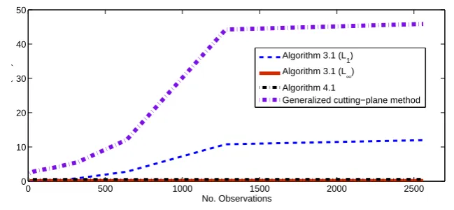
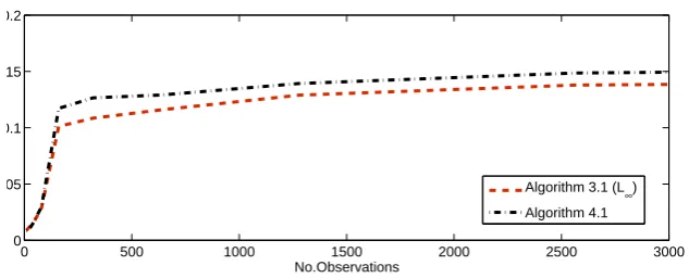
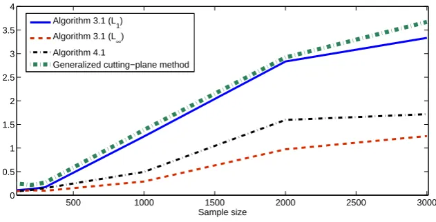
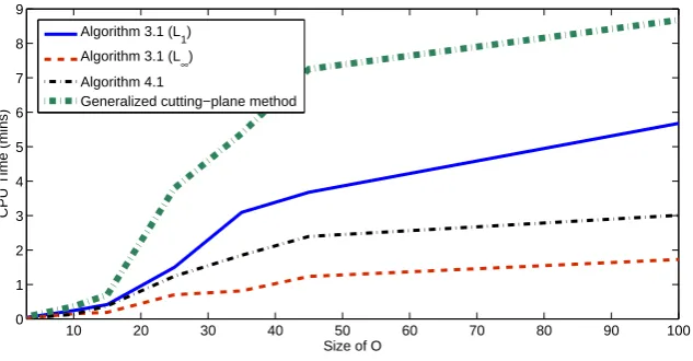
5. Numerical tests. In this section, we investigate the numerical performance of Algorithms 3.1 and 4.1 along with the generalized cutting-plane method. We do so by applying them to an academic problem, a practical portfolio selection problem and a supply chain problem.
The tests are carried out in MATLAB 7.10 installed on a HP Notebook PC with Windows 7 operating system, Intel Core i7 processor. We use IBM ILOG CPLEX Studio 12.4 to solve the subproblems within the Algorithm 3.1 and the Algorithm 4.1, while the subproblem within the generalized cutting-plane method is solved by “fmincon” due to nonlinearity. Furthermore, Algorithm 3.2 is integrated in the Al-gorithm 3.1, to find a suitable penalty parameter. The initial penalty parameter is set as 100. For Algorithm 3.1, we use the stopping criteria parametersϵ= 10−4and τ= 0.5. Moreover, the Algorithm 4.1 and the generalized cutting-plane method pro-posed in [8] terminates when the solution of any subproblem become a feasible point of the original problem, see Step 3 of Algorithm 4.1 for details.
Example 5.1. Consider problem (2.5) withF(x, ξ) =−xξ,G(x, ξ) =xξ−12x2, Y(ξ) = G(1, ξ), X = [0,50], where ξ is a random variable with finite distribution P(ξ= 2 + i−N1) = N1 fori= 1,· · ·, N and N= 101. The problem can be specifically presented as:
min
x −
1 101
101
∑
i=1
x(2 +i−1 101 ),
s.t. 1 101
101
∑
i=1
(η−x(2 +i−1 101 ) +
1 2x
2) +≤
1 101
101
∑
i=1
(η−(2 +i−1 101 ) +
1
2)+,∀η∈IR, x∈ X.
(5.1) It is difficult to work out the feasible set precisely. Here we only need to find out the optimal solution of problem (5.1). Forx∈[1,3],
P(G(x, ξ)≤η)≤P(Y(ξ)≤η),for allη∈IR,
which meansG(x, ξ)≽1G(1, ξ), and henceG(x, ξ)≽2G(1, ξ). Whenx >3,
N
∑
i=1
pi(1.5−G(x, ξi))+>
N
∑
i=1
which impliesG(x, ξ)̸≽2G(1, ξ). This shows that any point in the interval [1,3] is a feasible point of problem (5.1) whereas any pointxwithx >3 is infeasible. It is easy to see thatx∗ = 3 is the optimal solution (with corresponding optimal value −7.5) because the objective function is linear w.r.t. x.
We apply the L1-norm based penalty scheme (3.6) and L∞-norm based penalty scheme (3.9) to problem (5.1) respectively. To justify the application, we examine the SCQ of problem (5.1) and estimate the penalty parameter ρ. Consider formulation (2.7) for problem (5.1). Lety:= minNi=1Y(ξi). It is easy to show thaty=Y(2). For
x0= 2, it is a feasible point. Moreover, G(x0, ξ)≽1 Y(ξ), andG(x0, ξi)> y for all i= 1,· · · , N. This verifies the conditions of Theorem 2.1. Hence formulation (2.7) of problem (5.1) satisfies the SCQ.
Next we estimate the penalty parameter ρ through Theorem 3.1. We need to work outκ, δ andD defined in Lemma 3.1. Observe first that the objective function of problem (5.1) is Lipschitz continuous function with modulusκ= 3. Let
δ:=− max
j∈{1,...,N}
(
1 N J ∈Nmax
∑
i∈J
(Yj−G(x0, ξi))− 1 N
N
∑
i=1
(Yj−Y(ξi))+
)
.
It is easy to calculate thatδ= 0.005. On the other hand, it is easy to verify that the feasible set of problem (5.1) is contained in [0,3]. Let D= 3. We obtain an estimate of penalty parameterρ, that is,ρ > κδ−1D= 1800.
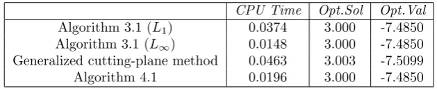
We have carried out numerical tests on four algorithms for problem (5.1): Algo-rithm 3.1 based on exact penalization with L1-norm (Algorithm 3.1 (L1) for short), Algorithm 3.1 based on exact penalization with L∞-norm ( Algorithm 3.1 (L∞) for short), Algorithm 4.1 and the generalized cutting-plane method.
The numerical results are displayed in Table 5.1. A few words about the notation.
Opt.Soldenotes the numerical optimal solution andOpt.Valdenotes the corresponding
[image:22.595.97.412.488.552.2]optimal value. To check the efficiency of the algorithms, we have recorded the CPU time (in minutes) for each of the algorithms.
Table 5.1
Numerical results for (5.1), Example 5.1.
CPU Time Opt.Sol Opt.Val
Algorithm 3.1 (L1) 0.0374 3.000 -7.4850
Algorithm 3.1 (L∞) 0.0148 3.000 -7.4850
Generalized cutting-plane method 0.0463 3.003 -7.5099
Algorithm 4.1 0.0196 3.000 -7.4850
The results show that all four algorithms perform efficiently albeit Algorith-m 3.1 (L1) and generalized cutting-plane method takes slightly more CPU time. To further investigate the performance of the algorithms, we propose to run a portfolio optimization problem of larger size.
Example 5.2. Consider a portfolio optimization problem with nonlinear
trans-action cost where short selling is allowed. Letrj: Ω→IR, denote the random return
rate of asset j forj = 1,· · ·, n,and R:= (r1, . . . , rn). We assume that E[|rj|]<∞.
Denoting by xj the fraction of the initial capital invested in asset j, we can easily
derive the total return rate: