Penalty-free multi-objective evolutionary approach to optimization of anytown water distribution network

Penalty-Free Multi-Objective Evolutionary Approach

to Optimization of Anytown Water Distribution Network

Calvin Siew1&Tiku T. Tanyimboh1&

Alemtsehay G. Seyoum1

Received: 31 August 2015 / Accepted: 20 May 2016

#The Author(s) 2016. This article is published with open access at Springerlink.com

Abstract This paper describes the development and application of a new multi-objective evolutionary optimization approach for the design and upgrading of water distribution systems with multiple pumps and service reservoirs. The optimization model employs a pressure-driven analysis simulator that accounts for the minimum node pressure constraints and conservation of mass and energy. Pump scheduling, tank siting and tank design are integrated seamlessly in the optimization without introduc-ing additional heuristic procedures. The computational solution of the optimization problem is entirely penalty-free, thanks to pressure-driven analysis and the inclusion of explicit criteria for tank depletion and replenishment. The model was applied to the Anytown network that is a benchmark optimization problem. Many new solutions were achieved that are cheaper and offer superior performance compared to previous solutions in the literature. Detailed and extensive simulations of the solutions achieved were carried out. Spatial and temporal variations in water quality were investigated by simulating the chlorine residual and disinfection by-products in addition to water age. The hydraulic requirements were satisfied; efficiency of pumps was consistently high; effective operation of the new and existing tanks was achieved; water quality was improved; and overall computational efficiency was high. The formulation is entirely generic.

Keywords Demand-driven analysis . Pressure-driven analysis . Penalty-free constrained multiobjective evolutionary optimization . Water distribution system . Optimal pump scheduling . Service reservoir design and operation

DOI 10.1007/s11269-016-1371-1

* Tiku T. Tanyimboh [email protected]

1

1 Introduction

A large proportion of the optimization models for water distribution systems focus on networks consisting of pipes only. Very few published works simultaneously incorporate the sizing and operation of tanks and pumps, multiple operating conditions and demand variations which are all typical features of water distribution systems. This is mainly attributed to the significant increase in complexity which stems from the additional design variables and multiple operational constraints. In addition, accurate dynamic simulation of the system is extremely time-consuming, particularly in evolutionary optimization algorithms that operate on large populations of candidate solutions.

The Anytown network is a hypothetical system with multiple loadings and multiple storage tanks and pumps (Walski1987). Murphy et al. (1994) applied an evolutionary algorithm to optimize the design based on single-objective optimization with constraint-violation penalties. Walters et al. (1999) solved the problem using multi-objective optimization. Dimensional weightings were required to facilitate the aggregation of the various system improvements considered. Vamvakeridou-Lyroudia et al. (2005) employed multi-objective optimization combined with fuzzy membership functions for constraint handling purposes based on aggregators that essentially are weightings. The performance is heavily dependent on the many parameters and operators introduced.

Several researchers modified the Anytown problem by incorporating other measures of hydraulic performance. Farmani et al. (2005,2006) considered the resilience index (Todini

2000) and water age (Rossman2002). Prasad and Tanyimboh (2008) investigated the statis-tical flow entropy (Tanyimboh and Templeman2000; Tanyimboh et al.2011) and resilience index. More recently Atkinson et al. (2014) maximized flow entropy and resilience index at once in an attempt to generate hybrid solutions with properties derived from the two measures. The above-mentioned extensions and other aspects such as the uncertainties associated with the nodal demands (Spiliotis and Tsakiris2012) were not considered in this article.

Kurec and Ostfeld (2013) addressed tank sizing for a network in the literature. They employed constraint-violation tournaments, and coefficients for tank-level imbalances. Con-straint handling methods in evolutionary algorithms generally employ penalties (e.g. Kougias and Theodossiou2013) or some form of weighting to standardize different constraint violation measures. The major disadvantage of using these parameters (Dridi et al.2008) is that there is no rigorous method to obtain their values. Users often have to find the most effective values by experimentation that is time consuming. Moreover, penalty parameters and weightings are often problem specific in that they may perform well on some problems but not so well on others. Hence the whole cycle of calibration and trial runs has to be repeated every time a different optimization problem is solved. In addition, the optimality of the solution heavily depends on these parameters.

This paper extends previous work by the authors that was concerned with the optimization of networks with pipes only (Siew and Tanyimboh 2012a; Siew et al.

Furthermore, optimal tank siting and pump scheduling are fully integrated in the opti-mization procedure. Upgrading of pumping stations and the operation and energy consumption costs are considered. This new formulation achieved many new solutions that are fully feasible, satisfy both pressure and other hydraulic and operational con-straints, and are cheaper than the previous solutions in the literature. The solutions achieved were assessed further, in terms of the fluctuations of the water levels in the tanks, plus the temporal and spatial variations of the water quality in the distribution system. Given the context of the Anytown network that is hypothetical, the values used in the water quality simulations were selected to achieve the prescribed minimum chlorine residual throughout the distribution system.

2 Brief Overview of Anytown Network Optimization Problem

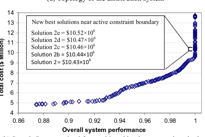
A brief summary of the network is presented here for completeness. The layout of the Anytown network is shown in Fig.1a. The source is a water treatment plant located at node 40 with a fixed water level of 3.05 m. Water is pumped from the plant into the system via three identical pumps operating in parallel. There are two existing storage tanks located at nodes 14 and 17 both with operating water levels between 68.58 m and 76.20 m. The volume of water below 68.58 m and above 65.53 m is emergency storage. Other data for pipes and nodes are available in Walski (1987).

A minimum pressure of 28.12 m must be provided at all nodes for theaverage day flowof 24 hours duration as well as theinstantaneous peak flow, i.e. 1.8 times the average day flow. There are three different critical fire flowsduring which water is supplied at a minimum pressure of 14.06 m. With one pump out of service and all tanks starting at their lowest operating levels for normal storage, the emergency storage in each tank must be sufficient for a 2-hour fire and at the same time supplypeak flow demands,i.e. 1.3 times the average day flow. 35 existing pipes are considered for paralleling or cleaning and lining. In addition, there are six new pipes to be sized. One or two new tanks can be added to the network. Potential tank locations can be any of the 16 available nodes which are not connected directly to an existing tank. Tanks are connected to a node by a riser of length 30.78 m with the diameter to be determined.

New pumping stations are not considered but an upgrade of the existing pumping station is allowed through the addition of one or two new pumps with identical characteristics to the existing ones. Given eight average-day demand factors (one each for the eight 3-hour durations in 24 hours), eight ON-OFF status control variables are used for the operation of a single pump. As such, each status control variable corresponds to a demand factor. This enables the pump scheduling to be optimized for the different demand periods.

3 Methodology for Tank Siting and Design

Tanyimboh2010a). This approach avoids the problems of tank flow imbalances (e.g. Murphy et al.1994; Walters et al.1999; Kurek and Ostfeld2013).

(a) Topology of the distribution system

Pipes laid in the residential area New pipes

4 5 6 7 8 9 10 11 12 13 14

0.86 0.88 0.9 0.92 0.94 0.96 0.98 1

Total cost ($ Million)

New best solutions near active constraint boundary

Solution 2e = $10.52×106

Solution 2d = $10.47×106

Solution 2c = $10.46×106

Soluon 2b = $10.44×106 Soluon 2 = $10.43×106

Overall system performance

(b) Sample Pareto-optimal front achieved by the proposed method

Fig. 1 The Anytown water distribution network. Solutions with system performance values less than unity are

Moreover, the philosophy here is different (Siew and Tanyimboh2010b). For example, constraints to balance the respective initial and final water levels in the tanks and are not required. Similarly, a constraint to balance the total inflow and outflow volumes of the tanks for the network as a whole is not required. In addition to pressure-driven extended-period simulation, we have incorporated criteria that promote tank depletion and replenishment in the objective function (Section 4). Accordingly, solutions having tanks with excessive cost, insufficient or excessive elevation, insufficient or excessive capacity, partial depletion or partial replenishment are optimized out seamlessly through natural selection. If a candidate solution has a new tank, the solution’s chromosome specifies the site and other relevant parameters. The pressure-driven hydraulic simulator together with penalty-free Pareto dominance permits any solution(feasible or infeasible)to be rated realistically and without bias.

It may be recalled that in extended-period simulation, a snapshot analysis is executed at the beginning of a hydraulic time step and the system is checked for any status changes during the hydraulic time step. If, for example, the water level in a new tank reaches the minimum level before the end of the time step, the tank’s riser is temporarily closed and an additional snapshot analysis is performed due to the changed system state. This sequence is carried out in each hydraulic time step in the extended-period simulation. This is the standard procedure for extended-period simulation in EPANET-PDX (a pressure-driven hydraulic simulation model developed in the present research) (Siew and Tanyimboh2010a,2012b). Conceptually the extended period simulation procedure is the same as in EPANET 2. Tank designs achieved at the end of the optimization are final and no further tank adjustments (as in e.g. Vamvakeridou-Lyroudia et al.2005) are required.

New tanks were assumed to be cylindrical. Four design variables for the new tanks were used as follows (Vamvakeridou-Lyroudia et al.2005; Prasad2010).

(a) Total volume (V);

(b) Ratio of diameter to height (D/H);

(c) Ratio of emergency volume to total volume (v/V); and (d) Level of the bottom of the tank (i.e. the tank’s elevation).

Upper and lower bounds on the shape parameterD/Hand emergency storage fractionv/V

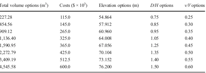
were employed to avoid solutions that may be undesirable in practice (Prasad2010). All nodes except those already connected directly to an existing tank were considered as possible locations for new tanks. Table 1 summarizes the decision variables of the optimization problem. The range of tank volumes and their associated costs was taken from Walski (1987). Intermediate tank sizes were considered here and corresponding costs were interpo-lated linearly. The tank-sizing decision variables were discretized to provide eight options per decision variable (Table2).

4 Formulation of the Optimization Model

Gupta and Bhave1996; Giustolisi et al.2008; Gorev and Kodzhespirova2013; Kovalenko et al.2014; Ciaponi et al.2015), is the ratio of the flow delivered to the flow required (Ackley et al.2001; Tanyimboh et al.2003; Kalungi and Tanyimboh2003; Tanyimboh and Templeman

2010). The demand satisfaction ratio is also known as the available demand fraction (see e.g. Abdy Sayyed et al.2015; Gupta2015).

The first objective functionf1represents the total cost while the second objective functionf2 represents the system’s performance;f1is minimized andf2is maximized.

f₁¼χ2 ð1Þ

f₂¼π4 ð2Þ

whereχandπare the normalised total cost and system performance functions, respectively. The exponents 2 and 4, in Eqs.1and2respectively, are default empirically derived values in Siew and Tanyimboh (2012a). For solutioni,

χi¼

Ci

Cmax;

i¼1; …; N I ð3Þ

whereNIis the number solutions,Ciis the total cost for solutioniandχiis the normalised total cost. This includes all the costs incurred (i.e. pipes, pumps, tanks, energy, etc.). The present

Table 1 Overview of the decision variables

Variables Explanations

Existing pipes 35 pipes to be considered for paralleling or cleaning and relining New pipes 6 pipes to be sized

Existing tanks Operation of 2 tanks to be optimized

New tanks Up to 2 tanks to be sized and located, and their operation optimized New tank risers Tank risers to be sized for the new tanks

Tank sizing parameters V,D/H,v/Vand elevation

Existing pumps Operation of 3 pumps to be optimized

New pumps Up to 2 pumps to be added to the station and their operation optimized Pump status 8 ON-OFF control variables per pump

Table 2 Tank costs and associated discrete decision variable options

Total volume options (m3_{) Costs ($ × 10}3_{) Elevation options (m) D/Hoptions v/Voptions}

227.28 115.0 54.864 0.75 0.25

454.56 145.0 57.912 0.85 0.30

909.12 265.0 60.960 0.95 0.35

1,136.40 325.0 64.008 1.05 0.40

1,590.95 365.0 67.056 1.25 0.45

2,272.79 425.0 70.104 1.35 0.50

3,409.19 512.5 73.152 1.40 0.55

4,545.58 600.0 76.200 1.50 0.60

worth of energy costs is based on an interest rate of 12 % and an amortisation period of 20 years. Details of the costs of pipe paralleling, cleaning and lining, pump operation and tanks are available in Walski (1987).Cmaxis the cost of the most expensive of solutions in the population.

We investigated two alternative definitions of the system performance functionπin Eq.2. For solutioni,whereNIis the number solutions,

πi¼ 1 2

1

N L

XN L

l¼1

μlþ 1

N R

XN R

r¼1

ρr !

; i¼1; …; N I ð4Þ

whereNLis the number of loading conditions (e.g. average day, peak flow, etc.),NRis the number of service reservoirs or tanks. For service reservoirr,ρris the replenishment ratio; i.e. the ratio of the volume of water at the end of the last hour of the extended-period simulation to the total operational water volume. This criterion aims to refill each reservoir at the end of the operational cycle (typically 24 hours). For loading condition l, μl is the average network demand satisfaction ratio; i.e. the ratio of the available flow to the demand and is derived from the pressure-driven simulation model. Maximizing this criterion aims to satisfy all the nodal demands (Ackley et al. 2001). In this way, the minimum node pressure constraints are addressed seamlessly (Siew and Tanyimboh2012a; Siew et al.2014).

The average network demand satisfaction ratioμlfor loading conditionlis

μl¼ 1

N Tl XN Tl

t¼1

σt; l¼1;…;N L ð5Þ

For hydraulic time stept,σtis the network demand satisfaction ratio; andNTlis the number of hydraulic time steps for loading conditionl.The parametersμl,ρrandσtall have values between 0 and 1. Hence, the system performance functionπi(Eq.4) reaches a maximum value of 1 when all the criteria defined are met. Asπicomprises normalised necessary conditions, additional weights or coefficients are not required.

The system performance functionπimay achieve fully feasible solutions. However, the solutions so obtained need not make full use of the variable storage of the service reservoirs during the average day. Therefore, to improve the formulation further, an additional criterion was introduced in Eq.6to promote service reservoir depletion.

πi¼ 1 3

1

N L

XN L

l¼1

μlþ 1

N R

XN R

r¼1

ρrþδr

!

; i¼1; …; N I ð6Þ

For service reservoirr,δris the depletion ratio i.e. the ratio of the maximum cumulative depletion achieved for the average-day flow to the total operational volume. This criterion promotes cost effectiveness and improves water quality through full depletion of the service reservoirs in each cycle (see e.g. Edwards and Maher2008).

5 Computational Solution of the Optimization Problem

optimization problem. PF-MOEA is based on NSGA II (non-dominated sorting genetic algorithm) (Deb et al. 2002). PF-MOEA rates all solutions according to the performance functionπi(Eq.4or6) followed by Pareto dominance based purely on the performance and cost functionsπiandχi.

The pressure-driven hydraulic simulator EPANET-PDX (Siew and Tanyimboh 2012b; Seyoum and Tanyimboh 2014) is embedded in PF-MOEA. The pressure-driven hydraulic simulator provides a realistic assessment of the hydraulic properties of the solutions with insufficient flow and pressure as it takes account of the relationship between the pressure at a demand node and the flow that is available (see e.g. Elhay et al.2016). Unlike NSGA II (Deb et al.2002), PF-MOEA rates both feasible and infeasible solutions strictly according to their cost effectiveness. Accordingly, in PF-MOEA all feasible and infeasible non-dominated

solutions are considered superior toall feasible and infeasible dominatedsolutions. In other words, non-dominated infeasible solutions are considered superior to dominated feasible solutions. Additional details on the methodology and its effectiveness are available in Siew and Tanyimboh (2012a) and Siew et al. (2014). Also, demonstrations of the effectiveness of an alternative penalty-free formulation that uses the EPANET 2 hydraulic simulator are available in Saleh and Tanyimboh (2013,2014,2016). The hydraulic modelling approach in EPANET 2 assumes that the flow that is available at a demand node is the same as the demand and is thus characterised as demand-driven analysis (see e.g. Spiliotis and Tsakiris2011).

We wrote the program for the genetic algorithm in C++ (Siew and Tanyimboh2012a). We used binary coding and the operators were single-bit mutation, single-point crossover and binary tournament selection for crossover. The population size was 200; crossover probability was 1; and mutation rate was 0.005; 15 optimization runs with different initial populations were conducted for each formulation (Eqs. 4 and 6) of the performance functionπi. The members of the initial populations were selected randomly except for the minimum and maximum solution vectors that are always included by default. Each decision variable in the minimum solution vector has the smallest permissible value within the solution space. Similarly each decision variable in the maximum solution vector has the largest permissible value within the solution space.

Each optimization run lasted 5,000 generations i.e. one million function evaluations. We carried out extended-period simulation with a hydraulic time step of one hour for the 24-hour average-day flow. Previous studies used hydraulic time steps of three hours (Vamvakeridou-Lyroudia et al. 2005; Prasad 2010) and six hours (Walters et al. 1999). Also, we used a hydraulic time step of 30 minutes for the fire flows. Apersonal computer(Intel Core 2 Duo, CPU 2.66 GHz, RAM 3.23 GB) was used for this study. A typical optimization run required on average 22.7 hours; i.e. 16.36 seconds per generation or 0.08 seconds per function evaluation.

6 Results and Discussion

constants of 0.5/day and 0.1 m/day, respectively, were assumed (Carrico and Singer2009). To ensure the chlorine residual at all demand nodes and tanks remained just above 0.2 mg/L (WHO2011) the chlorine concentration at the treatment plant was kept constant at 0.6 mg/L. A maximum total THM (trihalomethane) concentration of 100 μg/L (European 1998) was adopted. For water age and THM, initial values of zero were assumed for all nodes and tanks. The 72-hour extended-period simulation in EPANET 2 required 1.6 seconds for water age, 1.3 seconds for chlorine and 2 seconds for THM, on an Intel Xeon workstation(with two processors of CPU 2.4 GHz and RAM of 16 GB). To avoid misunderstanding, thisworkstation

was used for the water quality modelling only. The other aspects i.e. optimization and results verification were performed on the PC (personal computer) mentioned previously in Section 5.

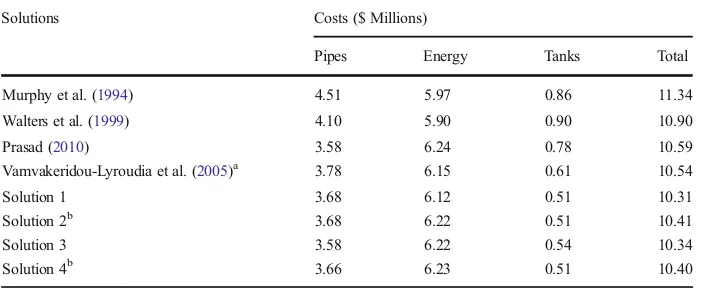
Two of the best solutions achieved i.e. Solutions 1 and 2, are presented and discussed in detail. These solutions are fully feasible as they do not violate any node pressure constraints while operating under all five loading conditions and all tanks fully refill for the average-day 24-hour cycle. Both solutions have been simulated with a hydraulic time step ofone minuteto confirm their feasibility. Figure1bshows the Pareto-optimal front from which Solution 2 was obtained. The optimization algorithm consistently found many feasible designs as in Fig.1b. Therefore, post-optimization, artificially stringent criteria were adopted for the hydraulic simulations of the solutions achieved. Aside from Solution 2, there are many fully feasible designs in the same optimization run that are cheaper than the previous best solution in the literature. Table3provides a cost comparison with the previous best solutions.

The algorithm also achieved consistently many competitive solutions that are feasible based on larger hydraulic simulation time steps of 30 or 60 minutes. Two such solutions, i.e. Solutions 3 and 4, from different optimization runs, are included for completeness but not discussed in detail. All solutions presented are cheaper than the cheapest feasible solution reported in the literature to date with a total cost of $10.59 million (Prasad2010). Solutions 1, 2 and 4 achieved the lowest tank costs compared to previous published solutions. The least cost solution achieved (Solution 1) has a total cost of $10.31 million. New pumps were not required and a single new tank was added.

Table 3 Cost comparison with previous best solutions

Solutions Costs ($ Millions)

Pipes Energy Tanks Total

Murphy et al. (1994) 4.51 5.97 0.86 11.34

Walters et al. (1999) 4.10 5.90 0.90 10.90

Prasad (2010) 3.58 6.24 0.78 10.59

Vamvakeridou-Lyroudia et al. (2005)a 3.78 6.15 0.61 10.54

Solution 1 3.68 6.12 0.51 10.31

Solution 2b _{3.68 6.22 0.51 10.41}

Solution 3 3.58 6.22 0.54 10.34

Solution 4b _{3.66 6.23 0.51 10.40}

a

Maximum velocity constraints were not considered herein as they are not in the original problem specification (Walski1987). However, all solutions presented have average day flows with velocities less than 2 m/s (Prasad2010). Take Solution 2 for instance whose maximum flow velocity is 1.51 m/s in pipe 4 at the 10th hour when the demand factor of 1.3 is the highest. Pipe 4 connects node 1 to the pumping station.

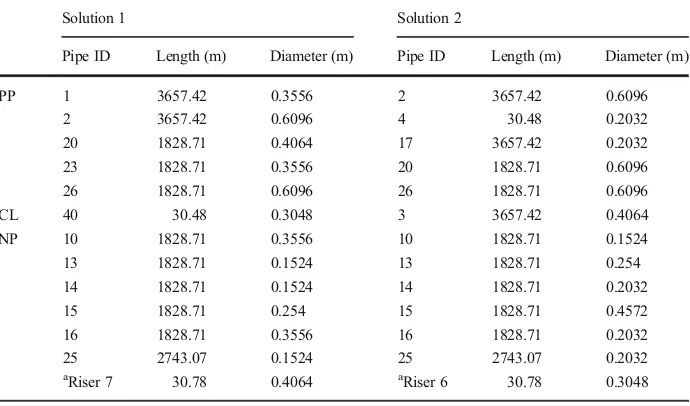
Pipe upgrading and rehabilitation details for the best two solutions are summarized in Table 4. The values of the pipe diameters in Table4 have been converted from inches to metres; the pipe sizes are in fact discrete. The results generally appear to suggest that pipe paralleling (PP) is preferred to cleaning and lining (CL). In each of Solutions 1 and 2, only one pipe was selected for cleaning and lining (Table4).

Table 4 Pipe upgrading and rehabilitation results

Solution 1 Solution 2

Pipe ID Length (m) Diameter (m) Pipe ID Length (m) Diameter (m)

PP 1 3657.42 0.3556 2 3657.42 0.6096

2 3657.42 0.6096 4 30.48 0.2032

20 1828.71 0.4064 17 3657.42 0.2032

23 1828.71 0.3556 20 1828.71 0.6096

26 1828.71 0.6096 26 1828.71 0.6096

CL 40 30.48 0.3048 3 3657.42 0.4064

NP 10 1828.71 0.3556 10 1828.71 0.1524

13 1828.71 0.1524 13 1828.71 0.254

14 1828.71 0.1524 14 1828.71 0.2032

15 1828.71 0.254 15 1828.71 0.4572

16 1828.71 0.3556 16 1828.71 0.2032

25 2743.07 0.1524 25 2743.07 0.2032

a

Riser 7 30.78 0.4064 aRiser 6 30.78 0.3048

1 in = 0.0254 m PP = Pipe paralleling CL = Pipe cleaning and lining NP = New pipes

a

Risers 6 and 7 are risers for new tanks located at nodes 6 and 7 respectively

Table 5 Properties of the new tanks

Properties Solution 1 Solution 2

Maximum operating water level (m) 72.98 72.98 Minimum operating water level (m) 67.18 66.56

Top level (m) 74.31 74.31

Bottom level (m) 60.96 60.96

Diameter (m) 18.67 18.67

Tank location Node 7 Node 6

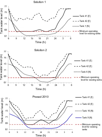
Solution 1 is the cheapest solution achieved at a total cost of $10.31 million. Unlike most previous solutions in the literature with two tanks (e.g. Prasad 2010), a single new tank was added at node 7 (Tank 7(N) hereafter). No new pumps were added to the pumping station. One of the three existing pumps operates when demands are high from 9 a.m. to 6 p.m. i.e. nine hours and the remaining two

67 69 71 73 75 77

Tank water level (m)

Time (h) Solution 1

Tank 41 (E)

Tank 42 (E)

Tank 7 (N)

Minimum operating level for existing tanks

67 69 71 73 75 77

Tank water level (m)

Time (h) Solution 2

Tank 41 (E)

Tank 42 (E)

Tank 6 (N)

Minimum operating level for existing tanks

67 69 71 73 75 77

6 9 12 15 18 21 24 3 6

6 9 12 15 18 21 24 3 6

6 9 12 15 18 21 24 3 6

Tank water level (m)

Time (h)

Prasad 2010 Tank 41 (E)

Tank 42 (E)

Tank 16 (N)

Tank 9 (N)

Minimum operating level for existing tanks

operate for the entire 24 hours. The pumps collectively use 18,733.5 kWh of energy per day (Table 5).

The pump operation strategy achieved is somewhat different from other solutions published in the literature (e.g. Walters et al. 1999) where the third pump is usually switched on during the low demand period to re-fill the tanks. Herein, for Solution 1, additional flow during the peak demand hours is supplied by both the new tank and the third pump. Probably this could be the reason why the algorithm only allocated one new

Table 6 Optimized pumping schedules

Solutions Number of pumps operating Energy consumption (kWh/day)

6–9 h 9–15 h 15–18 h 18–6 h

1 2 3 3 2 18,733.50

2a 3 3 2 2 19,017.92

a_{Solution with tank depletion criterion}

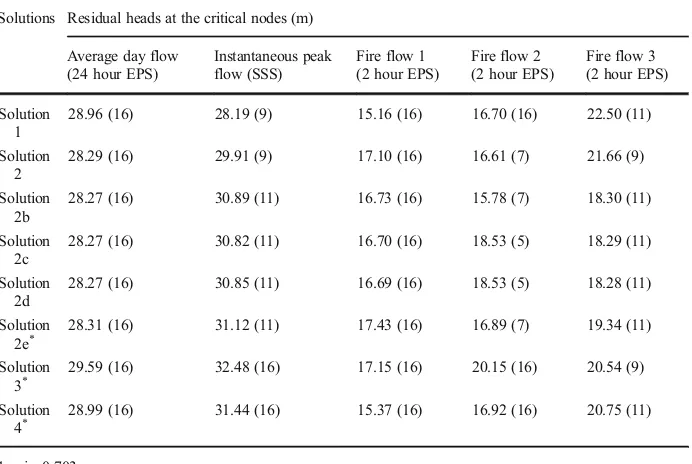
Table 7 Minimum pressures for the various loading conditions

Solutions Residual heads at the critical nodes (m)

Average day flow (24 hour EPS)

Instantaneous peak flow (SSS)

Fire flow 1 (2 hour EPS)

Fire flow 2 (2 hour EPS)

Fire flow 3 (2 hour EPS)

Solution 1

28.96 (16) 28.19 (9) 15.16 (16) 16.70 (16) 22.50 (11)

Solution 2

28.29 (16) 29.91 (9) 17.10 (16) 16.61 (7) 21.66 (9)

Solution 2b

28.27 (16) 30.89 (11) 16.73 (16) 15.78 (7) 18.30 (11)

Solution 2c

28.27 (16) 30.82 (11) 16.70 (16) 18.53 (5) 18.29 (11)

Solution 2d

28.27 (16) 30.85 (11) 16.69 (16) 18.53 (5) 18.28 (11)

Solution 2e*

28.31 (16) 31.12 (11) 17.43 (16) 16.89 (7) 19.34 (11)

Solution 3*

29.59 (16) 32.48 (16) 17.15 (16) 20.15 (16) 20.54 (9)

Solution 4*

28.99 (16) 31.44 (16) 15.37 (16) 16.92 (16) 20.75 (11)

1 psi = 0.703 m

The figures in parentheses represent the critical nodes i.e. the nodes with the smallest pressures

The required pressure is 28.12 m (40 psi) for average day and instantaneous peak flows; and 14.06 m (20 psi) for all fire flows

EPS - extended period simulation SSS - single snapshot simulation *

tank instead of two as in some of the previous solutions (Prasad 2010; Vamvakeridou-Lyroudia et al.2005; Murphy et al.1994).

Table5 provides details of the new tank. Figure 2ashows the tank operating levels over a cycle of 24 hours for the average day flow. All tanks refill fully by the end of the day. The new Tank 7(N) and existing Tank 41 (Tank 41(E) hereafter) drain rapidly (approximately 6 and 3 hours respectively). The water level in existing Tank 42 (Tank 42(E) hereafter) fluctuates and only approximately 40 % of the total operational volume is utilised. For comparison purposes, the tank operations from Prasad (2010) are presented also in Fig. 2c. It is evident that the capacity of Tank 42(E) is not fully utilised. Similarly, the best solution in Vamvakeridou-Lyroudia et al. (2005) has this weakness for the average day and two fire flows. The above-mentioned solutions including Solution 1 are thus undesirable from the standpoint of tank operation and water quality.

10 20 30 40 50

Water age (hours)

Time (hours) Exisng Tank 42

Soluon 1 Soluon 2

10 20 30 40 50

Water age (hours)

Time (hours) New Tanks 6 and 7

Tank 7 (N) Tank 6 (N)

0.2 0.3 0.4 0.5

Chlorine (mg/L)

Time (hours) Exisng Tank 42

Soluon 1 Soluon 2

0.2 0.3 0.4 0.5

Chlorine (mg/l)

Time (hours) New Tanks 6 and 7

Tank 7 (N) Tank 6 (N)

10 20 30 40 50 60

THM (ug/L)

Time (hours) Exisng Tank 42

Soluon 1 Soluon 2

10 20 30 40 50 60

6 9 12 15 18 21 24 3 6 6 9 12 15 18 21 24 3 6

6 9 12 15 18 21 24 3 6 6 9 12 15 18 21 24 3 6

6 9 12 15 18 21 24 3 6 6 9 12 15 18 21 24 3 6

THM (ug/L)

Time (hours) New Tanks 6 and 7

Tank 7 (N) Tank 6 (N)

Solution 2 costing $10.41 million was the cheapest feasible solution achieved with the enhanced performance function in Eq.6. One new tank was added at node 6, i.e. Tank 6(N). No new pumps were added; the pumping cost is slightly higher than Solution 1. All three pumps operate from 6 a.m. to 3 p.m. i.e. nine hours when the demands are high. Only two pumps are required for the rest of the day (Table 6). Costs for the new tank and pipe rehabilitation are similar to Solution 1.

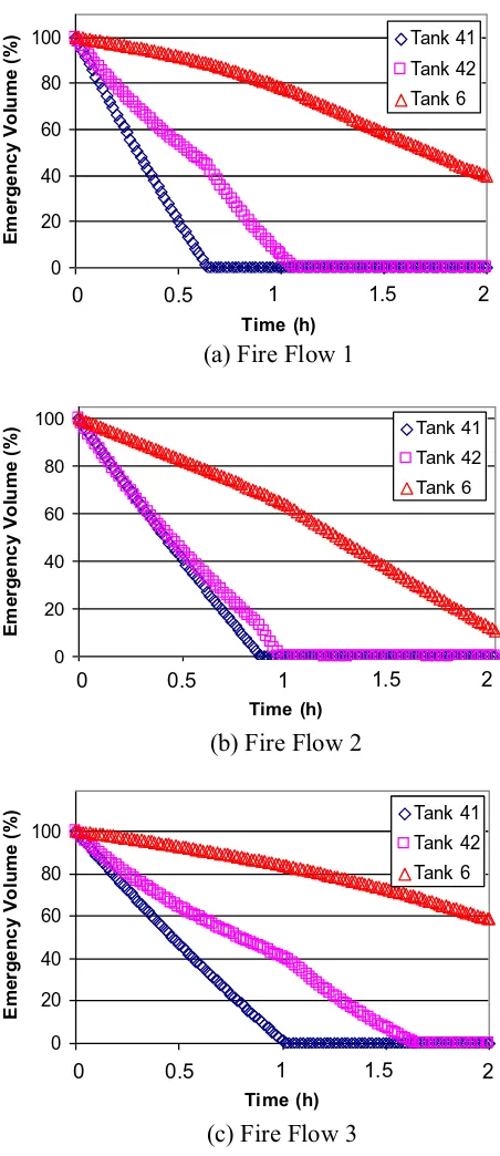
Figure2bshows the operation cycles of the tanks for the average-day flow for Solution 2. The available operational volumes for all three tanks are utilised effectively. Indeed the water level in existing Tank 42(E) reaches a minimum level of 0.21 m above the minimum operating level. This shows that the proposed new formulation in Eq.6with the tank depletion criterion is advantageous. TheAppendixshows the tank operations for the three fire flows. The total emergency storage provided by the tanks satisfies the fire flows. Existing Tanks 41(E) and 42(E) drain fully in each case. The new Tank 6(N) reaches a maximum depletion of approximately 90 % at the end of Fire-flow 2.

0 10 20 30 40

Water age (hours)

Demand nodes Soluon 1

0 10 20 30 40

Water age (hours)

Demand nodes Soluon 2

0.2 0.3 0.4 0.5 0.6 0.7

Chlorine (mg/l)

Demand nodes Soluon 1

0.2 0.3 0.4 0.5 0.6 0.7

Chlorine (mg/l)

Demand nodes Soluon 2

0 15 30 45 60

THM (μg/l)

Demand nodes Soluon 1

0 15 30 45 60

THM (μg/l)

Demand nodes Soluon 2

Table 7 provides the values of the pressures at the most critical nodes for the various loading conditions and shows that all the solutions satisfy the pressure requirements in full. Results presented herein are based on steady state and extended period simulations (with a hydraulic time step of one minute unless otherwise stated) performed with EPANET-PDX. Also, the solutions were re-checked in EPANET 2 that gave the same results. For theresults verification, a 24 hour extended-period simulation with a hydraulic time step of one minute took 0.843 seconds in EPANET-PDX on the PC.

Over the 24 hour cycle (with hydraulic time step of one minute) the pumps of Solution 1 operate consistently near their best efficiency point of 65 % and do not drop below 60.5 %. For Solution 2, the efficiency of the three pumps varies between 60 and 65 % throughout the 24 hour operating cycle. Aside from the ON-OFF status variables for pump scheduling in Table 1, no extraneous operational constraints were applied to the pumps. For example, Prasad (2010) and Vamvakeridou-Lyroudia et al. (2005) used a constraint on the pump operational capacity to meet daily demand variation.

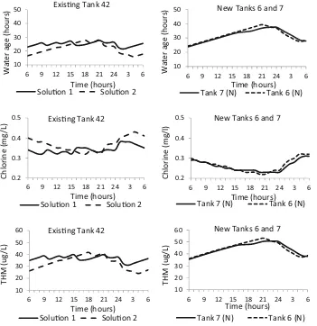
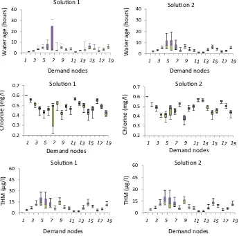
Finally, in terms of water quality, Fig. 3 shows the two new tanks 6(N) and 7(N) are generally comparable. On the other hand water quality is better in the existing Tank 42(E) in Solution 2 due to the criterion that promotes tank depletion. Also Fig. 4 suggests that in Solution 1 the water quality at node 7 would have the largest deviation from the average among all the demand nodes in both Solutions 1 and 2. These results seem to suggest that overall, considering both the tanks and demand nodes, Solution 2 is better. However, without additional investigations it is difficult to say whether the improved formulation of the performance functionπiin Eq.6is the most dominant factor. Figure5shows the depletion of the emergency storage for Solution 2, for the three fire-fighting flow scenarios.

7 Conclusions

This article concerns the development and application of a new multi-objective evolutionary optimization approach for the design and upgrading of water distribution systems with multiple pumps and service reservoirs. The tank siting and design methodology was based on pressure-driven extended-period simulation and was shown to be highly effective and the performance of the pumps was consistently efficient. Explicit criteria for the depletion and replenishment of the service reservoirs were included in the optimization model. The optimization procedure developed achieved many optimal and near optimal solutions consistently when applied to the benchmark Anytown water distribution network. The new best solutions found for the Anytown network were competitive and fully feasible. The advantages of the proposed new approach are that it is practical and generic.

Acknowledgments The authors are grateful to the UK Engineering and Physical Sciences Research Council

(EPSRC Grant Number EP/G055564/1), the British Government (Universities UK, Overseas Research Students’ Award Scheme) and the University of Strathclyde Glasgow for funding this research. This research was carried out in collaboration with Veolia (now Affinity) Water.

All relevant data are included in this paper.

Compliance with Ethical Standards

Appendix: Emergency Storage Depletion During Fire Flows

(a) Fire Flow 1

20 40 60 80 100

Time (h)

Emergency Volume (%)

Emergency Volume (%)

Emergency Volume (%)

Tank 41 Tank 42

Tank 6

0 0.5 1 1.5 2

(b) Fire Flow 2

20 40 60 80 100

Time (h)

Tank 41 Tank 42 Tank 6

0 0.5 1 1.5 2

(c) Fire Flow 3

20 40 60 80 100

Time (h)

Tank 41 Tank 42

Tank 6

0 0.5 1 1.5 2

Open AccessThis article is distributed under the terms of the Creative Commons Attribution 4.0 International License (http://creativecommons.org/licenses/by/4.0/), which permits unrestricted use, distribution, and repro-duction in any medium, provided you give appropriate credit to the original author(s) and the source, provide a link to the Creative Commons license, and indicate if changes were made.

References

Abdy Sayyed MA, Gupta R, Tanyimboh TT (2015) Noniterative application of EPANET for pressure dependent modelling of water distribution systems. Water Resour Manag 29(9):3227–3242. doi:10.1007/s11269-015-0992-0

Ackley JRL, Tanyimboh TT, Tahar B, Templeman AB (2001) Head-driven analysis of water distribution systems. Water Softw. Sys.: Theory and Applications, Vol. 1, Ulanicki, B., Coulbeck, B., and Rance, J. (eds.), Research Studies Press Ltd, England, ISBN 0863802745, Chapter 3:183–192

Atkinson S, Farmani R, Memon FA, Butler D (2014) Reliability indicators for water distribution system design: comparison. J Water Resour Plan Manag 140(2):160–168

Carrico B, Singer PC (2009) Impact of booster chlorination on chlorine decay and THM production: simulated analysis. J Environ Eng 135(10):928–935

Ciaponi C, Franchioli L, Murari E, Papiri S (2015) Procedure for defining a pressure-outflow relationship regarding indoor demands in pressure-driven analysis of water distribution networks. Water Resour Manag 29:817–832. doi:10.1007/s11269-014-0845-2

Deb K, Pratap A, Agarwal S, Meyarivan T (2002) A fast and elitist multiobjective genetic algorithm: NSGA-II. Evol Comp, IEEE Trans 6(2):182–197

Dridi L, Parizeau M, Maihot A, Villeneuve J-P (2008) Using evolutionary optimization techniques for scheduling water pipe renewal considering a short planning horizon. Comput-Aided Civ Infrastruct Eng 23(8):625–663 Edwards J, Maher J (2008) Water quality considerations for distribution system storage facilities. Am Water

Works Assoc J 100(7):60

Elhay S, Piller O, Deuerlein J, Simpson A (2016) A robust, rapidly convergent method that solves the water distribution equations for pressure-dependent models. J. Water Resour Plan Manag 142(2). doi:10.1061/ (ASCE)WR.1943-5452.0000578

European Community (1998) Council Directive 98/83/EC on the quality of water intended for human consump-tion. Official Journal of the European Communities L330

Farmani R, Walters GA, Savic DA (2005) Trade-off between total cost and reliability for Anytown water distribution network. J Water Resour Plann Manag 131(3):161–171

Farmani R, Walters GA, Savic DA (2006) Evolutionary multi-objective optimization of the design and operation of water distribution network: total cost vs. reliability vs. water quality. J Hydroinform 8:165–179 Giustolisi O, Savic DA, Kapelan Z (2008) Pressure-driven demand and leakage simulation for water distribution

networks. J Hydraul Eng 134(5):626–635

Gorev NB, Kodzhespirova IF (2013) Noniterative implementation of pressure-dependent demands using the hydraulic analysis engine of EPANET 2. Water Resour Manag 27(10):3623–3630

Gupta R (2015) History of pressure-dependent analysis of water distribution networks and its applications. World Environ Water Resour Congress 2015:755–765. doi:10.1061/9780784479162.070

Gupta R, Bhave PR (1996) Comparison of methods for predicting deficient network performance. J Water Resour Plann Manag 122(3):214–217

Kalungi P, Tanyimboh TT (2003) Redundancy model for water distribution systems. Reliab Eng Syst Saf 82(3):275–286 Kougias IP, Theodossiou NP (2013) Multi-objective pump scheduling optimization using harmony search

algorithm and polyphonic HSA. Water Resour Manag 27(5):1249–1261

Kovalenko Y, Gorev NB, Kodzhespirova IF, Prokhorov E et al (2014) Convergence of a hydraulic solver with pressure-dependent demands. Water Resour Manag 28:1013–1031

Kurek W, Ostfeld A (2013) Multi-objective optimization of water quality, pumps operation, and storage sizing of water distribution systems. J Env Manag 115:189–197

Murphy LJ, Dandy GC, Simpson AR (1994) Optimum design and operation of pumped water distribution systems. Proc Hydraul Civil Eng Conf, Institution of Engineers, Brisbane, Australia, 149–155

Prasad TD (2010) Design of pumped water distribution networks with storage. J Water Resour Plann Manag 136(1):129–132

Prasad TD, Tanyimboh TT (2008) Entropy based design of“Anytown”water distribution network. Proc 10th Ann Water Distrib Syst Anal Conf, ASCE/EWRI, Kruger National Park, South Africa, 450–461. doi:10. 1061/41024(340)39

Saleh HSA, Tanyimboh TT (2013) Coupled topology and pipe size optimization of water distribution systems. Water Resour Manag 27(14):4795–4814. doi:10.1007/s11269-013-0439-4

Saleh SHA, Tanyimboh TT (2014) Optimal design of water distribution systems based on entropy and topology. Water Resour Manag 28(11):3555–3575

Saleh SHA, Tanyimboh TT (2016) Multi-directional maximum-entropy approach to the evolutionary design optimization of water distribution systems. Water Resour Manag 30(6):1885–1901. doi: 10.1007/s11269-016-1253-6

Seyoum AG, Tanyimboh TT (2014) Pressure dependent network water quality modelling. J Water Manag 167(6):342–355. doi:10.1680/wama.12.00118

Siew C, Tanyimboh TT (2010a) Pressure-dependent EPANET extension: extended period simulation. 12thInte Conf Water Distrib Syst Anal, ASCE/EWRI, Tucson, Arizona, USA, 85–95. doi:10.1061/41203(425)10

Siew C, Tanyimboh TT (2010b) Penalty-free multi-objective evolutionary optimization of water distribution systems. 12th_{Int Conf Water Distrib Syst Anal, ASCE/EWRI, Tucson, Arizona, USA, 764–770. doi:10.} 1061/41203(425)71

Siew C, Tanyimboh T (2012a) Penalty-free feasibility boundary-convergent multi-objective evolutionary algo-rithm for the optimization of water distribution systems. Water Resour Manag 26(15):4485–4507 Siew C, Tanyimboh TT (2012b) Pressure-dependent EPANET extension. Water Resour Manag 26(6):1477–1498 Siew C, Tanyimboh T, Seyoum A (2014) Assessment of penalty-free multi-objective evolutionary optimization approach for the design and rehabilitation of water distribution systems. Water Resour Manag 28(2):373–389 Spiliotis M, Tsakiris G (2011) Water distribution system analysis: Newton-Raphson method revisited. J Hydraul

Eng ASCE 137(8):852–855

Spiliotis M, Tsakiris G (2012) Water distribution network analysis under fuzzy demands. Civ Eng Environ Syst 29(2):107–122

Tanyimboh T, Templeman A (2000) A quantified assessment of the relationship between the reliability and entropy of water distribution systems. Eng Optim 33(2):179–199

Tanyimboh TT, Templeman AB (2010) Seamless pressure-deficient water distribution system model. J Water Manag 163(8):389–396. doi:10.1680/wama.900013

Tanyimboh TT, Tahar B, Templeman AB (2003) Pressure-driven modelling of water distribution systems. Water Sci Technol–Water Supply 3(1–2):255–261

Tanyimboh TT, Tietavainen MT, Saleh SHA (2011) Reliability assessment of water distribution systems with statistical entropy and other surrogate measures. Water Sci Technol–Water Supply 11(4):437–443 Todini E (2000) Looped water distribution networks design using a resilience index based heuristic approach.

Urban Water 2(3):115–122

Vamvakeridou-Lyroudia LS, Walters GA, Savic DA (2005) Fuzzy multiobjective optimization of water distri-bution networks. J Water Resour Plann Manag 131(6):467–476

Walski TM (1987) Discussion of multi-objective optimization of water distribution networks. Civ Eng Syst 4(1): 215–217

Walters GA, Halhal D, Savic D, Ouazar D (1999) Improved design of“Anytown”distribution network using structured messy genetic algorithms. Urban Water 1(1):23–38