Modelling wave-current interactions off the east coast of Scotland

www.ocean-sci.net/12/875/2016/ doi:10.5194/os-12-875-2016

© Author(s) 2016. CC Attribution 3.0 License.

Modelling wave–current interactions off the east coast of Scotland

Alessandro D. Sabatino1, Chris McCaig1,a, Rory B. O’Hara Murray2, and Michael R. Heath1 1_{Marine Population Modelling Group, Department of Mathematics and Statistics,}

University of Strathclyde, Glasgow, UK

2_{Marine Scotland Science, Marine Laboratory, Aberdeen, UK} a_{now at: Brookes Bell, 280 St. Vincent Street, Glasgow, UK}

Correspondence to:Alessandro D. Sabatino ([email protected]) Received: 20 November 2015 – Published in Ocean Sci. Discuss.: 18 December 2015 Revised: 14 April 2016 – Accepted: 15 April 2016 – Published: 5 July 2016

Abstract.Densely populated coastal areas of the North Sea are particularly vulnerable to severe wave conditions, which overtop or damage sea defences leading to dangerous flood-ing. Around the shallow southern North Sea, where the coastal margin is lying low and population density is high, oceanographic modelling has helped to develop forecasting systems to predict flood risk. However, coastal areas of the deeper northern North Sea are also subject to regular storm damage, but there has been little or no effort to develop coastal wave models for these waters. Here, we present a high spatial resolution model of northeast Scottish coastal waters, simulating waves and the effect of tidal currents on wave propagation, driven by global ocean tides, far-field wave con-ditions, and local air pressure and wind stress. We show that the wave–current interactions and wave–wave interactions are particularly important for simulating the wave conditions close to the coast at various locations. The model can simu-late the extreme conditions experienced when high (spring) tides are combined with sea-level surges and large Atlantic swell. Such a combination of extremes represents a high risk for damaging conditions along the Scottish coast.

1 Introduction

Due to its semi-enclosed morphology and shoaling bathymetry, the North Sea experiences extreme wave condi-tions, in particular during winter periods (Woolf et al., 2002). When combined with sea-level surges such events can lead to damaging inundation of low-lying coastal regions, due to

wave overtopping of sea defences. Development of a mod-elling and predictive capability for high-resolution wave con-ditions in the North Sea is therefore a high priority. How-ever, the task is complicated due to interaction between lo-cally generated waves and incoming swell from outside the region, and especially due to interactions between waves and tidal currents.

Crossing, or bimodal, sea states occur between 5 and 40 % of the time in the North Sea (Guedes Soares, 1984). These are generated when swell waves propagating into the re-gion from distant storm events interact with locally generated waves which may be of very different direction, period, and height. Swell waves from the North Atlantic and the Norwe-gian Sea propagate into the North Sea, interacting with local wind-sea-generated waves, modifying the main spectral pa-rameters. The interaction between differing wave trains is not fully understood, but crossing seas have been statistically as-sociated with freak wave incidence, and shipping accidents (Waseda et al., 2011; Tamura et al., 2009; Cavaleri et al., 2012; Onorato et al., 2006, 2010; Sabatino and Serio, 2015; Toffoli et al., 2011a). The North Sea is particularly prone to rogue wave events, such as the famous Draupner wave recorded in 1994 (Haver, 2004), the first ever recorded rogue wave event, that occurred in crossing sea conditions (Adcock et al., 2011). In the paper, the effect of the enhancement of the wind-sea waves due to swell is assessed during storms.

study carried out by Tolman (1991) highlighted that WCIs are significant in the North Sea, changing the significant wave height (Hs) and the mean wave period (Tm) by 5 and 10 %, respectively, during storm periods. However, the model that was used by Tolman (1991) to assess this effect was at very course resolution and broad scale. In particular, the ef-fect of the WCI in the coastal shallow areas was not con-sidered. Phillips (1977) showed that in the absence of wave breaking, local wave amplitude is given by

A A0

=√ c0

c(c+2U ), (1)

whereA is the resulting wave amplitude,A0 is the unper-turbed amplitude of the wave field,cis the wave phase speed, andU is the current that interacts with the wave train. It is important to notice that the sign of the current is determinant on the effect of the WCI: if the current travels in opposite di-rection with the wave train, there will be an enhancement of the significant wave height. Conversely, if current and waves are in the same direction, theHs decreases. For deep water waves, the phase speedcdepends only on the period of the wave, while in shallow watercdepends only on the depth. Equation (1) shows that the waves travelling in a direction opposing the current (U <0) have a positive ratioA/A0and consequently, an enhancement of the wave amplitude.

WCIs could also lead to the breaking of the wave: if the current is strong enough to block the wave train (Ris and Holthuijsen, 1996), these waves can break and lose energy before arriving to the coastline (Chawla and Kirby, 2002, 1998).

WCIs are particularly difficult to quantify empirically, and computationally intensive to model. In addition, the WCIs are a well-known mechanism for the formation of rogue waves in the ocean: the Agulhas current, that flows near the coastline of South Africa, was one of the first places in which this mechanism was identified (Mallory, 1974; Lavrenov, 1998; Lavrenov and Porubov, 2006). Recently, many studies (Onorato et al., 2011; Toffoli et al., 2013, 2015; Shrira and Slunyaev, 2014; Ma et al., 2013) highlighted that the interac-tion between a train of waves with an adverse current could increase its wave steepness, and cause rogue waves due to the modulational instability (Benjamin and Feir, 1967). How-ever, it is clear that shallow coastal waters, embayments, and headlands are particular foci for interactions (Hearn et al., 1987; Signell et al., 1990a). Model studies have concentrated on comparing wave height and period in coupled and uncou-pled model versions showing, for example, 3 % difference in wave height and 20 % in wave period in the Dutch and Ger-man coastal waters of the North Sea (Osuna and Monbaliu, 2004). Similar results have been obtained for coastal wa-ters of the Adriatic during bora conditions (Benetazzo et al., 2013), finding a maximum reduction for theHs of 0.6 m in the central Adriatic and a simultaneous increase up to 0.5 m in the gulfs of Trieste and Venice. WCIs were also studied

during hurricane conditions off the eastern seaboard of the USA (Xie et al., 2008).

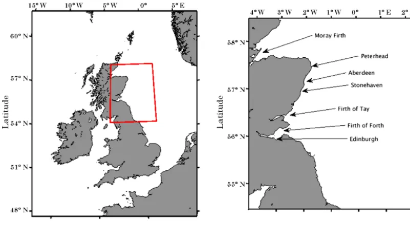
Sea defences of coastal settlements along the northeast coast of Scotland have suffered several damaging events dur-ing the period 2009–2014 as a result of surges and waves. The coastal waters are dominated by strong tidal currents and wind-driven residuals, are exposed to wave trains enter-ing the North Sea from the north, and generated by storm events in the central and southern North Sea. Although the oceanography of the North Sea as a whole has been inten-sively studied since the 1830s (Whewell, 1830; Proudman and Doodson, 1924; Dietrich, 1950; Huthnance, 1991; Otto et al., 1990), and the region was one of the earliest to be sub-jected to computational hydrodynamic modelling (Flather, 1987; Davies et al., 1985), high-resolution modelling activity has been largely concentrated in areas with potential for wave and tidal energy extraction (Adcock et al., 2013; Bryden and Couch, 2006; Baston and Harris, 2011; Shields et al., 2011, 2009). However, there are no such models for the northeast coast of mainland Scotland, and none which include coupled WCIs. Our objective here was to develop and test such a model for the stretch of coastline between the Firth of Tay and Peterhead, centred on the strategically important port city of Aberdeen and the town of Stonehaven (Fig. 1). The latter is the base for a governmentally supported marine mon-itoring site with a>15-year time series of high-resolution data on a wide range of environmental parameters (Bresnan et al., 2009).

2 Materials and methods

The MIKE by DHI model was used to simulate the tidal-and wind-driven circulation, tidal-and the wave propagation. The MIKE software is composed of different modules, for the creation of a model grid and input files and to simulate differ-ent hydrodynamical features at the same time or separately. The following modules were used:

– The MIKE Zero modules for generating the computa-tional grid and the input files.

– The MIKE 3 FM module for simulating the tidal and the wind-driven circulation.

– The MIKE 21 SW module for modelling the wave prop-agation.

For the simulation of the WCIs, a one-way coupling be-tween MIKE 3 FM and MIKE 21 SW was set up. The depth average flow fields and the water level output from MIKE 3 FM was provided as input to the MIKE 21 SW model. 2.1 The computational grid

Figure 1.The area studied in the present paper.

Figure 2.The computational grid generated with MIKE Zero soft-ware.

2002). Unstructured grids can represent complex coastlines better than a rectangular grid and potentially provide more realistic flows, enabling the geography of the coastline to affect the propagation of tidal and surface waves in a re-alistic manner. In addition, triangular grid elements allow

smoothly changing cell sizes across a region, with the highest resolution concentrated in an area of particular interest. The mesh for the area of study is shown in Fig. 2. An enhanced-resolution area was created near Stonehaven, because this work is part of a wider study focusing on the resuspension of the sediments in this part of the domain. This high-resolution area also covered the Firth of Forth and the Aberdeenshire coastline, where previous studies have shown enhanced cur-rents due to interaction between the tidal wave and the Scot-tish coastline (Dietrich, 1950; Otto et al., 1990).

2.2 The MIKE 3 FM hydrodynamic model

MIKE 3 FM (flow model) is based on the numerical solution of the 3-D incompressible Reynolds-averaged Navier–Stokes equations, under the Boussinesq and the hydrostatic pres-sure approximations (DHI, 2011a). The spatial discretization of the primitive equations is performed using a cell-centred finite-volume method. In the finite-volume method the vol-ume integrals in the partial differential equations with a di-vergence are converted to surface integrals using the Gauss– Ostrogradsky theorem (Toro, 2009).

MIKE 3 FM has a flexible approach for simulating the flow in the water column. It is possible to choose between sigma layers (Song and Haidvogel, 1994), z layers, and coupled sigma and z layers. For our purpose we decided to use the equidistant sigma layers approach, because the bathymetry of the area was not sufficiently complex to re-quire a more accurate description with a coupled sigma and

The coupled sigma andzlayers were tested, but there was no significant improvement for simulating the flow.

For the horizontal eddy viscosity the formulation proposed by Smagorinsky (1963) was used, in which the sub-grid-scale transport is expressed by an effective eddy viscosity related to a characteristic length scale rather than a constant eddy viscosity. This sub-grid-scale viscosity is given by

A=c_s2l2p2SijSij, (2)

wherecs is the Smagorinsky constant,lis the characteristic length of the grid size, and the deformation rate is given by (Lilly, 1966; Deardorff, 1971; Smagorinsky, 1963)

Sij =

1 2 _∂u i ∂xj + ∂uj ∂xi . (3)

The bed resistance was parameterized using a constant quadratic drag coefficientcf. The average bottom stress is

determined by a quadratic friction law: ¯

τb=cfρ0u¯b| ¯ub|, (4)

whereu¯bis the average flow velocity above the bottom and ρ0is the density of the water. The value of the above param-eters chosen for the model are reported in Sect. 3.1.

The model was forced with a time series of tidal elevations at the open boundaries from the open-source OSU (Oregon State University) Tidal Prediction Software (OTPS) (Egbert et al., 2010), based on TOPEX satellite observation of the water-level observations interpolated with tide gauge data from the European shelf region. In order to take account of the wind-driven circulation and surge in the model, meteoro-logical forcing was applied across the model domain, using the ERA-Interim reanalysis for wind velocity and mean sea-level pressure (Dee et al., 2011).

2.3 The MIKE 21 SW wave model

The MIKE 21 SW (spectral wave) is an unstructured grid model for wave prediction and analysis (DHI, 2011b). The MIKE 21 SW is based on the wave action conservation equa-tion (Komen et al., 1996; Young, 1999), where the dependent variable is the frequency-directional wave action spectrum. This is given by

∂N

∂t + ∇ ·(cN )= S

σ, (5)

whereSis the energy source term, defined as

S=Sin+Snl+Sds+Sbot+Ssurf (6)

that depends on the energy transfer from the wind to the wave fieldSin, on the nonlinear wave–wave interactionSnl, on the dissipation due to depth-induced wave breakingSsurf, on the dissipation due to bottom frictionSbot, and on the dissipation caused by the white-cappingSds.

The wave action density spectrum N(σ,θ) is defined as (Bretherton and Garrett, 1968)

N (σ, θ )=E(σ, θ )

σ , (7)

whereE is the wave energy density spectrum, σ=2πf is the angular frequency (wherefis the frequency), andθis the direction of wave propagation. The momentum transfer from the wind to the waves follows the formulation in Komen et al. (1996). The momentum transfer and the drag depend not only on the strength of the wind but also on the wave state itself.

For the physics of the propagation and breaking of the waves we choose the following parameters:

– The depth-induced wave breaking is based on the for-mulation of Battjes and Janssen (1978), in which the gamma parameter is a constant 0.6 across the domain. The formulation of the depth-induced wave breaking can be written as

Ssurf(σ, θ )= −

αQbσ H¯ m2 8π

E(σ, θ ) Etot

, (8)

whereα≈1.0 is a calibration constant,Qbis the frac-tion of breaking waves,σ¯ is the spectrum average fre-quency,Etotis the total wave energy that is linked to the wave action density spectrum, andHmis the estimated maximum wave height, that is defined as Hm=γ d (Battjes and Janssen, 1978), in whichdis the depth and

γis the free breaking parameter (Battjes, 1974). – The bottom friction is specified in the model as the

Nikuradze roughness (kN) (Nikuradse, 1933; Johnson and Kofoed-Hansen, 2000).

– The white-capping formulation described in Komen et al. (1996) in order to consider the dissipation of waves, based on the theory of Hasselmann (1974). For the fully spectral formulation, the white capping as-sumes a form that is dependent on the mean frequency

¯

σand on the wavenumberk:

Sds(σ, θ )= −Cds

¯

k2m0 2

"

(1−δ)k_¯ k+δ

_k ¯

k 2#

¯

σ N (σ, θ ). (9)

Here the two parameters,Cdsandδ, are the two dissipa-tion coefficients that control the overall dissipadissipa-tion rate and the strength of dissipation in the energy/action spec-trum, respectively, andm0is the zeroth moment of the overall spectrum.

The model also included nonlinear energy transfer such as the quadruplet wave interaction (Komen et al., 1996) and the triad wave interaction which is the dominant nonlinear interaction in shallow water (Eldeberky and Battjes, 1995, 1996).

The forcings included in the model are the local wind and the swell wave field from outside the model area and specified at the model boundaries. For the model bound-aries we used boundary conditions from the Venugopal and Nemalidinne (2014, 2015) North Atlantic model, a larger wave model that encompass the southern Norwegian Sea and the North Atlantic Ocean. The ERA-Interim 0.125◦×0.125◦ model was used to provide a wind field across the model do-main with a time resolution of 6 h (Dee et al., 2011; Berris-ford et al., 2011).

2.4 Wave–current interactions

The WCIs are implemented using a one-way coupling be-tween currents and waves. The model was run without and with currents implemented, and then the differences between the two runs were studied. The WCIs in the MIKE model are taken in account in the dispersion relation for the angular frequency term, since the current due by tides and wind af-fect the propagation and changes the wavelength of the wave train. The MIKE 21 SW dispersion relation in fact is

σ =pgktanh(kd)=ω−k·U . (10)

The one-way coupling has, however, some limitations since it is not taking into account the modification of the cur-rent by the wave itself (Michaud et al., 2011; Bennis et al., 2011).

2.5 Swell detection

In the present study, the wind-sea and the swell waves and their interaction are studied. MIKE 21 SW gives the oppor-tunity to separate spectrally the windsea waves and the swell waves. There are two criteria, based on a dynamic threshold, available to make this separation.

The first criterion is based on the difference of the energy between the spectrum and the fully developed sea condition (Earle, 1984). In this case, the threshold frequency is identi-fied as

fthreshold=αfp,PM _E

PM

EModel β

, (11)

whereα=0.7,β=0.31,EModelis the total energy at each node point calculated by the MIKE 21 SW model, and the Pierson–Moskowitz peak frequency and the energy are esti-mated as

fPM=0.14 g U10

(12)

EPM= _U

10

1.4g 4

. (13)

The second method is based on the wave-age criterion (Drennan et al., 2003) from empirical wave measurements in wave tanks and in Lake Ontario field measurements. From Donelan et al. (1985), swell waves are the components ful-filling the following relation:

U10 cp

cos(θ−θw) <0.83, (14)

whereU10 is the wind speed at 10 m,cpis the phase speed, θ is the wave propagation direction, andθw is the direction of the wind. For discriminate swell and windsea waves we used the second method, since it is the most widely used for this purpose and is the more reliable method (Drennan et al., 2003).

2.6 Validation data sets

The model was validated using five independent data sets. The hydrodynamic model was validated using data from the UK National Tide Gauge Network in Aberdeen and Leith and using the tide gauge data from the Scottish Environ-mental Protection Agency (SEPA) in Buckie. Validation was performed comparing harmonic components extracted from time series of both model and real data. The harmonic com-ponents of the sea level were extracted using the UTide Mat-lab function (Codiga, 2011).

Current meter observations from the British Oceano-graphic Data Centre (BODC) were used to validate the mod-elled currents. For the wave model, we compared recorded data from wave gauges in the Moray Firth and in the Firth of Forth (obtained from CEFAS) and data from a wave rider buoy deployed in Aberdeen Bay (data obtained from Uni-versity of Aberdeen). In addition, we used significant wave height and mean wave period from satellite data provided by WaveNet (CEFAS) for June 2008. Especially important in this case is the Aberdeen wave gauge, since this is the only one in shallow water (the depth of the sea in the mooring lo-cation is 10 m). This allows us to evaluate the ability of the model in coastal areas, in which the WCIs are strongest.

Table 1 shows details of the observations used for validat-ing and calibratvalidat-ing the tidal and wave model, while in Fig. S1 in the Supplement we show the position of the tide and wave gauges used for the validation and the position of the satellite data.

The validation for waves was carried out using four statis-tical indices: the bias, the root mean square error (RMSE), the correlation coefficient (R), and the scatter index (SI). These indices are defined below.

Bias= 1

N N X

i=1

xoi−xmi (15) RMSE= v u u t 1 N N X

i=1

xoi−xmi 2

Table 1.Location of the validation/calibration instrumentation.

Description Coordinates Depth (m) Use

longitude (◦) latitude (◦)

Aberdeen tide gauge −2.0803 57.144 – water level val/cal Leith tide gauge −3.1682 55.9898 – water level validation Buckie tide gauge −2.9667 57.6667 – water level validation Firth of Forth buoy −2.5038 56.1882 – waves validation Moray Firth buoy −3.3331 57.9663 – waves val/cal Aberdeen wave rider −2.0500 57.1608 – waves validation BODC 4551 RCM −2.8000 57.7910 12 current validation BODC 4561 RCM −1.9680 57.2320 12 current validation BODC 4562 RCM −1.9680 57.2320 27 current validation BODC 4571 RCM −1.9020 57.2260 12 current validation BODC 4572 RCM −1.9020 57.2260 52 current validation BODC 4582 RCM −2.1500 56.9870 23 current validation BODC 4591 RCM −2.0980 56.9820 12 current validation BODC 4592 RCM −2.0980 56.9820 47 current validation

R=

N P

i=1

xoi−xo

xmi−xm

s N P

i=1

xoi−xo 2

xmi−xm 2

(17)

SI=RMSE

xo

(18) For tidal current validation we used, instead of the SI, the normalized root mean square error (NRMSE), that is defined as

NRMSE= RMSE

max(x)−min(x). (19)

The validation was performed for different years. For the hydrodynamic model the agreement between modelled and observed water level was evaluated for the entire year 2007, while the currents were validated for 1992, where the rotor current meter observations were available. The wave model was validated for 2010 and 2008, where observations and boundary inputs were available.

3 Results

3.1 Calibration and validation of the hydrodynamic model

The hydrodynamic model was calibrated for the year 2007, based on the agreement with the recorded water level at the tide gauge in Aberdeen. The calibration parameters were the time step that was fixed at 1 s after an analysis of the Courant–Friedrichs–Lewy (CFL) conditions (higher time steps were investigated but the model was unstable); the Smagorinsky constant that was set to 0.2 (for values >0.3 the model showed some blow-up); and the bottom rough-ness that was parameterized with the drag coefficient cf =

Table 2.Computed RMSE for the main harmonic components, the validation for each tide gauge is reported in the Table S1.

Components RMSE

A (cm) g (◦)

M2 2.52 0.78

S2 1.64 3.68

N2 1.31 3.02

O1 0.76 5.42

K₁ 0.44 14.4

Q1 0.42 13.6

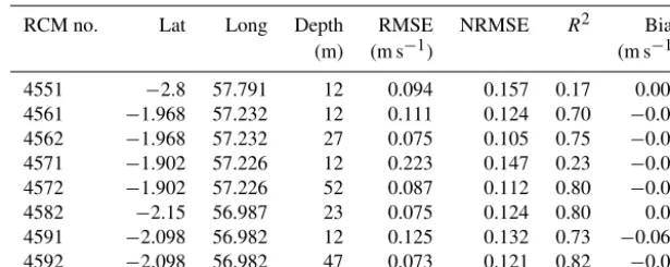
Table 3.Results from the validation of the currents, showing the difference between the modelled and observed current speeds at the eight locations reported in Table 1.

RCM no. Lat Long Depth RMSE NRMSE R2 Bias (m) (m s−1) (m s−1)

4551 −2.8 57.791 12 0.094 0.157 0.17 0.001 4561 −1.968 57.232 12 0.111 0.124 0.70 −0.03 4562 −1.968 57.232 27 0.075 0.105 0.75 −0.02 4571 −1.902 57.226 12 0.223 0.147 0.23 −0.05

4572 −1.902 57.226 52 0.087 0.112 0.80 −0.02

4582 −2.15 56.987 23 0.075 0.124 0.80 0.02 4591 −2.098 56.982 12 0.125 0.132 0.73 −0.062 4592 −2.098 56.982 47 0.073 0.121 0.82 −0.05

3.2 Calibration and validation of the wave model The calibration of the wave model was carried out for 3 months in 2008 and was based on the agreement between the observed and the modelledHsof the Firth of Forth wave gauge. There were three calibration parameters: the wave-breaking parameterγand the two dissipation coefficients as-sociated to the wave breaking (Cdisandδ). During this proce-dure we noticed how the most sensible parameter was theγ

controlling the wave breaking. We investigated the behaviour of the γ for the range 0.6–1.0, since most of the observa-tion studies in literature were reporting such values (Battjes, 1974; Stive, 1985; Battjes and Stive, 1985; Nelson, 1987, 1994; Kaminsky and Kraus, 1993), and we found thatγ= 0.6 was the value giving better results for theHs. The wave-breaking dissipation coefficients were fixed toCdis=2.5 and δ=0.8, while the Nikuradze bottom roughness was fixed to 0.01 m. The results of the wave gauges and satellite valida-tion are reported in Table 4. We evaluated the performance of the wave model with WCIs implemented (coupled) and without WCIs (uncoupled). There was a good agreement be-tween the modelled-with-WCI and measured wave data. The bias does not exceed 0.15 m for significant wave height. Ta-ble 4 and Fig. 3 shows that the model estimates correctly the significant wave height in the Firth of Forth and in Ab-erdeen but underestimates this parameter in the Moray Firth. However, the agreement with the data is still satisfactory. In particular, low RMSE values were recorded for the Ab-erdeen wave gauge, which is the only coastal shallow-water wave gauge that is available in the area (the depth of the mooring site is 10 m). The model performance against satel-lite data randomly sampled throughout the domain shows good agreement. Without the WCI included in the model, small or no differences were estimated for significant wave height, but larger differences were seen for mean wave pe-riod (Tm01=2π m0/m1): the calculated RMSE for the un-coupled model was 0.97 s in Aberdeen, 1.24 s in the Firth of Forth and 1.83 s in the Moray Firth. Comparing satellite observations in spring and winter conditions, it is possible to conclude that, in general, the model provides accurate

predic-Figure 3.Comparison between observed and modelledHsin the Firth of Forth and the Moray Firth for 2010.

tions for wave heights<1.5–2 m, but slightly underestimates the height of larger waves. On the other hand, wave periods are better modelled in the winter period when the waves are higher. No or very small differences were recorded between the coupled and uncoupled models for satellite validation. This is because the resolution of the satellite data is low and because the satellite data are often in deep water, where the WCI are less important.

3.3 Wave–current interaction

Table 4.Comparison between observed and modelled (both with and without WCIs implemented) wave heights and periods for wave gauges and satellite observations. The reported validation was carried out for 2010 (Firth of Forth and Moray Firth) and for 2008 (Aberdeen wave gauge and satellite observations). Details of the observation data are reported in Table 1 of the paper and in Table S2 of the Supplement.

Coupled Uncoupled

Bias RMSE R SI Bias RMSE R SI Firth of Forth

Hs −0.02 m 0.30 m 0.941 0.27 −0.01 m 0.30 m 0.939 0.27 Tm −0.70 s 1.17 s 0.767 0.25 −0.76 s 1.24 s 0.758 0.27 Moray Firth

Hs −0.14 m 0.42 m 0.849 0.38 −0.15 m 0.42 m 0.848 0.39 Tm −1.18 s 1.75 s 0.668 0.39 −1.23 s 1.83 s 0.656 0.41 Aberdeen

Hs −0.07 m 0.21 m 0.836 0.32 −0.07 m 0.22 m 0.831 0.32 Tm −0.25 s 0.91 s 0.715 0.20 −0.30 s 0.97 s 0.701 0.21 Satellite

Winter

Hs −0.2 m 0.4 m – 0.25 −0.2 m 0.4 m – 0.25 Tm +0 s 0.8 s – 0.15 +0 s 0.8 s – 0.15 Spring

Hs −0.1 m 0.3 m – 0.21 −0.1 m 0.3 m – 0.21 Tm +0.1 s 1.2 s – 0.23 +0.1 s 1.2 s – 0.23

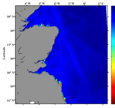
Figure 4.Root mean square difference between wave model output with and without WCI:(a)significant wave height (m),(b)peak wave period (s),(c)wave directional spreading (degrees).

Results show some differences between the two runs. In par-ticular, the largest deviations due to WCI are found in coastal areas, such as around headlands and bays, and in estuaries, in which the currents (mostly driven by tides) are strongest. As expected, the highest differences were seen in the proximity of the coastline (Signell et al., 1990b): this was because the strength of the mainly tidal-driven currents are stronger (Di-etrich, 1950; Otto et al., 1990). During spring tides, higher values for the current were recorded off northeast England and near Peterhead and Aberdeen (see Fig. 1). Wave periods are more affected than wave heights in this coupling, with rms deviations that can be on average 20 % (absolute value) in shallow-water coastal areas. We also considered the effect of the WCIs on the wave directional spreading, as this is an important variable for the stability of the wave train in deep water and for its evolution (Benjamin and Feir, 1967). The

results showed that during the 7-month period the significant wave height was, on average, less affected than directional spreading or wave periods: the difference was of the order of magnitude of 0.1 m near the coastline and less offshore, while the difference in peak spectral wave period (Tp) ex-ceeded 1 s in some of the east coast firths such as the Moray Firth and the Firth of Forth.

Pe-Figure 5.Maximum modelled positive deviation of theHs(m) due to the WCIs recorded in the 7-month period run in 2010.

terhead and south of the Firth of Forth, in which the tidally driven current is stronger (Dietrich, 1950; Otto et al., 1990). 3.4 Current and swell effect on the windsea wave field In order to study the importance of the WCIs and the cou-pling between swell and windsea waves off the east coast of Scotland, three storms were considered in the period January–August 2010. Storm events were identified by ex-amining the time series in the Firth of Forth and the Moray Firth in which the highest Hs were recorded. These three storms were selected because they were the three most in-tense storms during the considered period and originated from different weather conditions.

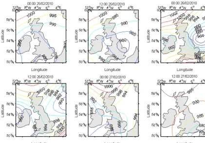
3.4.1 The 26–27 February 2010 storm

Between 25 and 27 February 2010, the UK was affected by a low pressure system, that moved rapidly from west to east. From the afternoon of the 25th to the 26th, the centre of the storm was over the North Sea (Fig. 7). At the same time, another low pressure system (not shown in the map) was over the Norwegian Sea, causing a train of swell moving from north to south. Comparison of modelled and observa-tion wave heights and wave period condiobserva-tions for this storm are reported in Fig. 8. In addition, the modelled conditions in the Aberdeen wave rider location are reported. The figure shows that the model reproduces adequately the conditions during that storm, in particular around the time in which the maximumHswas reached.

The low pressure over North Sea caused windsea waves exceeding 4 m. In Fig. 9 the situation in the sea is shown at

Figure 6.Maximum modelled negative deviation of theHs(m) due to the WCIs recorded in the 7-month period run in 2010.

12:30 UTC of the 26th: swell waves contributed to enhancing theHsin the centre of the storm, while a train of swell waves was forming from this storm, travelling west to the Moray Firth. Interaction of the windsea and the swell waves caused high waves along the east coast: the maximum recordedHs by the Firth of Forth wave gauge was 4.8 m. WCI contributed to the enhancement ofHsby up to 1 m in coastal areas, while in the open sea the contribution was very low, up to 0.1 m. In the afternoon of the 26th (Fig. 10, at 19:00 UTC) the storm was near the Firth of Forth. The contribution of the swell waves was significant, increasing theHsby up to 1 m: model outputs showed that the central part of the storm had anHs> 5 m, while without the swell coming from north the centre of the storm would have been anHs<4.5 m. To our knowledge, no significant damages were recorded for this storm. 3.4.2 The 30–31 March 2010 storm

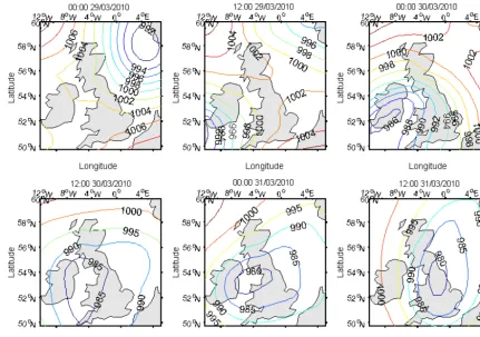
Figure 7.The mean sea level pressure fields (hPa) before and during the 25–26 March 2010 storm.

above the south of Scotland during the night between 30 and 31 March 2010. This depression generated both very high waves (Hs exceeded 6 m, measured in the Firth of Forth) and surge waves exceeding 0.5 m (measured both by the Ab-erdeen and Leith tide gauges). The waves caused signifi-cant damages to the coastal defences of cities in the south-east of Scotland. In particular, the City of Edinburgh Coun-cil estimated the damages to coastal defences to be about GBP 23 000. Also, in Berwick, at the southern entrance of the Firth of Forth, some damages were caused to the har-bour infrastructures. To the east, in Dumbar, waves topped the roofs of two-floor houses.

Damaging conditions associated with this storm were caused by a combination of simultaneous factors: (1) tides in the spring period, (2) a surge wave of about 0.5 m gener-ated by local pressure and wind, (3) windsea waves genergener-ated locally that interacted with strong currents, (4) a weak but significant swell waves field that interacted with the windsea waves.

Figure 12 shows the intensity of the current in the Ab-erdeen wave gauge location and the resulting WCI. It can be seen that the current was strongly enhanced by the wind, and consequently the WCI effect was stronger.

At about 00:30 UTC on 31 March 2010, the storm was at its maximum, causing the wave field to hit the coastline at around the same time as high tide and surge. The different

propagat-Figure 8.Wave conditions during the 25–26 February 2010 storm:

(a)comparison between coupled and uncoupled modelledHs(m) with observed data in Firth of Forth wave gauge;(b)comparison between coupled and uncoupled modelledHs(m) in the Aberdeen wave gauge; no observation data were available from this wave gauge during this storm;(c)comparison between coupled and un-coupled modelledTm(s) with observed data in Firth of Forth wave gauge;(d)comparison between coupled and uncoupled modelled Tm(s) in the Aberdeen wave gauge, no observed data were avail-able from this wave gauge during this storm.

ing outside the centre of the windsea waves to the coastline.

Hs recorded by the Firth of Forth wave gauge measured a peak of significant wave height of 6.46 m at 05:00 UTC on 31 March 2015. The model matched the peak recorded in the wave gauge reasonably well, predicting higher S values of the Firth of Forth, where more damages were caused. The wave–wave interactions due to the interaction between swell and windsea waves was important for the enhancement of theHsin the northern part of the Scotland, where the wind-sea wave conditions were less intense, while the contribution was low in the central part of the storm.

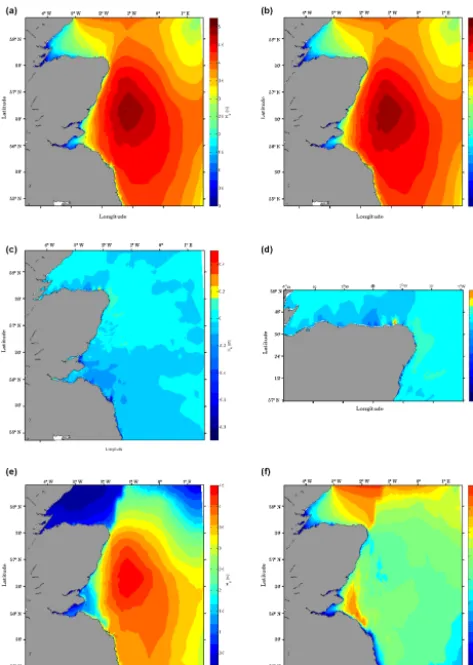
Figure 9. The modelled Hs on the east coast of Scotland at 12:30 UTC on 26 February 2010:(a)coupled model (mean WCI included),(b)uncoupled model (mean WCI not included),(c) dif-ference between coupled and uncoupled models,(d)difference be-tween coupled and uncoupled models in the Moray Firth area,

(e)windsea waves,(f)swell waves.

3.4.3 The 19 June 2010 storm

Figure 10. The modelled Hs on the east coast of Scotland at 19:00 UTC on 26 February 2010: (a)coupled model (mean WCI included),(b)uncoupled model (mean WCI not included),(c) dif-ference between coupled and uncoupled models,(d)difference be-tween coupled and uncoupled models in the Moray Firth area,

(e)windsea waves,(f)swell waves.

location is shown (Fig. 17b–d). The model demonstrates the wave conditions present during this storm well (both for wave heights and periods) and the results show the limited effect of the WCI in those locations. This field of waves ar-rived at the Scottish coastline at the same time as the low pressure was generating high waves in the bulk of the North Sea, causing two trains of waves to be in the same place at the same time. This condition, known as crossing or bi-modal sea, is quite common in the North Sea (Guedes Soares, 1984). The model hindcasted that the storm offshore was at its maximum near 16:00 UTC on 19 June 2010 (Fig. 18). At 16:00 UTC on 19 June 2010, the modelled offshore, mid-North Sea, windsea-generated waves peaked at Hs∼ 5 m (Fig. 14e), whereas the swell waves were a little smaller with

Hs∼3–4 m (Fig. 18f). Further north, in the Moray Firth, the swell waves dominated with the swell havingHs∼6 m and the windsea havingHs∼2 m. The resulting predicted wave field hadHs>6 m (Fig. 18b). In the Moray Firth, anHsof

more than 5 m was recorded. However, at this time, the cou-pling between currents and waves caused a decrease of the significant wave height at the coastline (Fig. 18c). In some locationsHswas reduced by more than 0.5 m (see Fig. 18c– d). Three hours later (Fig. 19), the turning tidal currents en-hanced the waves by more than 1.5 m in coastal locations. In this storm, the WCIs play a role in the enhancement of the wave conditions: spatially, the effect (Figs. 18–19) is signif-icant on the coastline. In addition, the windsea wave field is significantly enhanced by swell waves, and the bimodal sea conditions are effective in changing theHsdue to the inter-actions between swell and windsea waves.

3.5 Effect of WCI on the wave spectra

Considering the second storm (30–31 March 2010) we anal-ysed the effect of the WCI on the 1-D and 2-D spectra. Mod-elled spectra were extracted from the model output in three locations in correspondence with the wave gauges, and the output with and without WCIs was analysed (Figs. 20–22). Some significant variation of the energy density of the spec-tra (≈20 %) were seen for the considered storm, in particular for the Aberdeen wave gauge, but also for the Firth of Forth wave gauge, in which high waves were recorded; the major changes were reported near the spectral peak. The model also predicted a shift of the spectral peak and variation in swell magnitude. Since large variations were recorded for the Ab-erdeen wave gauge and the Firth of Forth wave gauge, we analysed the modelled directional spectra with and without WCIs for the considered storm. In Figs. 23–24, we show the results for the 2-D spectrum, in which not only the distribu-tion of the energy with the frequency was shown but also the distribution with the angle. Variation in the magnitude of the spectral energy with the angle along with small variation in the direction of the wave train were modelled.

Similar results for the spectrum variations are reported in Rusu (2010) for the WCIs at the mouth of Danube, while similar spectral changes were identified in laboratory experi-ments, as in Toffoli et al. (2011b) and Toffoli et al. (2015).

4 Conclusions

In this study we presented a model capable of hindcasting surge and storms on the east coast of Scotland. The combi-nation of spring tide, strong wind, and high waves can be ex-tremely threatening in coastal areas. The North Sea is one of the areas most affected by this forcings. Storms in North Sea can generate extremely high waves as well as rogue waves (Ponce de León and Guedes Soares, 2014).

Figure 11.The mean sea level pressure fields (hPa) before and during the 30–31 March 2010 storm.

world, such as in the southern North Sea (Osuna and Mon-baliu, 2004), in which the difference based on the normalized rms difference of a 1-month period is about 3 % for theHs and has an rms of 20 % forTm(Tables 3 and 4 of Osuna and Monbaliu, 2004). Such is the case in the northern Adriatic Sea in the shallow areas between the Venetian Lagoon, the Gulf of Trieste, and the Istrian peninsula, where deviations up to 1 m were modelled during bora and sirocco conditions (Benetazzo et al., 2013).

The validation shows that the model performs reasonably well during both calm periods and storms for waves, and also performs well for tides and surges.

During severe storms, in particular when the low pressure was over England and Scotland, it was found that the WCIs are significant, causing an increase or decrease inHsthat can exceed 2 m in some coastal areas, depending on the direction of the wave field compared to the current. A similar result was found for the peak spectral wave period: Fig. 4 shows that in the time period considered here the largest deviation of wave periods due to WCI is in the estuarine areas of the east coast, with rms deviations of more than 1.2 s.

Wave propagation in the Firth of Forth during storms gen-erated in the mid-North Sea is driven by trains of swell waves detaching from the open sea storm. During the stormy peri-ods considered here, the windsea waves in the Firth of Forth

did not exceed 3.5 m in the outer area of the estuary and 1 m in the inner part, while the swell field exceeded 5 m at the en-trance of the Firth of Forth. In the inner firth, the swell waves have a similar magnitude to the windsea waves. Conversely, the area of the estuary of the Firth of Forth is mainly driven by locally generated waves. A similar behaviour was noticed in the other two estuarine areas on the east coast: the Tay estuary and the Moray Firth.

The northeast coast of Scotland is more exposed to swell arriving from the North Atlantic and the Norwegian Sea, while the central and southern parts are more exposed to lo-cal windsea waves and to storms generated in the bulk of the North Sea.

Figure 12.Modelled currents and waves conditions in the Aberdeen wave gauge location during the 30–31 March 2010 storm (depth of the mooring location is 10 m).

and the current fields were only due by tides and the local field of wind and pressure. This led to an overall underesti-mation of the strength of the current and a possible underes-timation of the total effect of the WCI.

The model also has forecasting capabilities, in particular when nested with large-scale models, such as the North At-lantic model (Venugopal and Nemalidinne, 2014, 2015). A limitation of the model is that the MIKE by DHI software does not allow an online coupling between waves and tides, slowing the simulation process. In fact, currents and waves are simulated by different modules and it is not possible to perform a direct coupling. For this work, the currents were simulated first and then the output data were saved in order to use them as input for the wave model. Another limita-tion of the model, due to the one-way coupling, is that we can not study the effect of the wave setup and setdown on the surge water level (Longuet-Higgins and Stewart, 1962; Bowen et al., 1968), and most importantly, the wave radiation effect on the current field itself (Bennis et al., 2011; Michaud et al., 2011). Previous work on this interaction shows that the modification of the current field is more important in very shallow water areas (<10 m depth). In this paper, however,

Figure 13.The modelled surge wave due to the local wind and pres-sure at 02:00 UTC on 31 March 2010.

we were more interested in the effect of the current field on the wave. Future work will focus on understanding what ef-fect the waves have on the current dynamics on the east coast of Scotland. This will be implemented by first running the wave model, then using the wave radiation in the hydrody-namic model to estimate the enhancement of the water level due to waves near the shoreline and to estimate the variation of the current due to the wave radiation stress.

Figure 14. The modelled Hs on the east coast of Scotland at 00:30 UTC on 31 March 2010:(a)coupled model (mean WCI in-cluded),(b) uncoupled model (mean WCI not included),(c) dif-ference between coupled and uncoupled models,(d)difference be-tween coupled and uncoupled models in the Firth of Forth area,

(e)windsea waves,(f)swell waves.

Figure 15. The modelled Hs on the east coast of Scotland at 02:00 UTC on 31 March 2010:(a)coupled model (mean WCI in-cluded),(b) uncoupled model (mean WCI not included), (c) dif-ference between coupled and uncoupled models,(d)difference be-tween coupled and uncoupled models in the Firth of Forth area,

Figure 17. Wave conditions during the 19 June 2010 storm:

(a)comparison between coupled and uncoupled modelledHs(m) with observed data in Firth of Forth wave gauge;(b)comparison between coupled and uncoupled modelledHs(m) in the Aberdeen wave gauge, no observed data were available from this wave gauge during this storm;(c)comparison between coupled and uncoupled modelledTm(s) with observed data in Firth of Forth wave gauge;

(d) comparison between coupled and uncoupled modelledTm (s) in the Aberdeen wave gauge, no observed data were available from this wave gauge during this storm.

Figure 18. The modelled Hs on the east coast of Scotland at 16:00 UTC on 19 June 2010:(a)coupled model (mean WCI in-cluded),(b) uncoupled model (mean WCI not included), (c) dif-ference between coupled and uncoupled models,(d)difference be-tween coupled and uncoupled models in the Firth of Forth area,

Figure 19. The modelled Hs on the east coast of Scotland at 19:00 UTC on 19 June 2010: (a)coupled model (mean WCI in-cluded),(b) uncoupled model (mean WCI not included),(c) dif-ference between coupled and uncoupled models,(d)difference be-tween coupled and uncoupled models in the Firth of Forth area,

(e)windsea waves,(f)swell waves.

Figure 20. Modelled 1-D spectrum in the Firth of Forth wave gauge, the red line is the coupled model (with WCIs incorporated), while the blue line is the uncoupled model:(a)31 March 2010 at 00:30,(b) 31 March 2010 at 01:15,(c)31 March 2010 at 02:00,

(d) 31 March 2010 at 04:15, (e) 31 March 2010 at 06:00, and

Figure 21.Modelled 1-D spectrum in the Moray Firth wave gauge, the red line is the coupled model (with WCIs incorporated), while the blue line is the uncoupled model: (a) 31 March 2010 at 00:30,(b) 31 March 2010 at 01:15,(c)31 March 2010 at 02:00,

(d) 31 March 2010 at 04:15, (e) 31 March 2010 at 06:00, and

(f)31 March 2010 at 08:30 UTC.

Figure 22.Modelled 1-D spectrum in the Aberdeen wave gauge, the red line is the coupled model (with WCIs incorporated), while the blue line is the uncoupled model: (a) 31 March 2010 at 00:30,(b) 31 March 2010 at 01:15,(c)31 March 2010 at 02:00,

(d) 31 March 2010 at 04:15, (e) 31 March 2010 at 06:00, and

Figure 23. Polar plot of the modelled 2-D directional spec-trum (energy density, m2×s/degrees) in the Firth of Forth wave gauge, red indicates the contour plot of the coupled model spectrum (with WCIs incorporated), while black indicates the contour plot of the uncoupled model. Contour lines are plot-ted every 0.01 m2s degrees−1: (a) 31 March 2010 at 00:30,

(b) 31 March 2010 at 01:15, (c) 31 March 2010 at 02:00,

(d) 31 March 2010 at 04:15, (e) 31 March 2010 at 06:00, and

(f)31 March 2010 at 08:30 UTC.

Figure 24.Polar plot of the modelled 2-D directional spectrum (en-ergy density, m2×s/degrees) in the Aberdeen wave gauge, red in-dicates the contour plot of the coupled model spectrum (with WCIs incorporated), while black indicates the contour plot of the uncou-pled model. Contour lines are plotted every 0.01 m2s degrees−1:

(a) 31 March 2010 at 00:30, (b) 31 March 2010 at 01:15,

(c) 31 March 2010 at 02:00, (d) 31 March 2010 at 04:15,

The Supplement related to this article is available online at doi:10.5194/os-12-875-2016-supplement.

Acknowledgements. The authors wish to acknowledge Ian

Thurl-beck, Robert Wilson, Alessandra Romanó, Reddy Nemaliddine, Vengatesan Venugopal, Jon Side, Arne Vogler, Ruari MacIver, Simon Waldman, and the two anonymous reviewers for their helpful suggestions. The authors are grateful for the financial support of the UK Engineering and Physical Sciences Research Council (EPSRC) through the TeraWatt: Large-scale interactive coupled 3-D modelling for wave and tidal energy resource and environmental impact consortium. The authors are also grateful to Cefas (UK) for providing satellite and wave gauge data, to Thomas O’Donoghue for providing the Aberdeen Bay wave buoy data, to the British Oceanographic Data Center (BODC) and the Scottish Environmental Protection Agency (SEPA) for the tide gauge and RCM data, and to the European Centre for Medium-Range Weather Forecasts (ECMWF) for providing wind and pressure data.

Edited by: A. Sterl

References

Adcock, T., Taylor, P., Yan, S., Ma, Q., and Janssen, P.: Did the Draupner wave occur in a crossing sea?, P. Roy. Soc. Lond. A-Conta., 467, 3004–3021, 2011.

Adcock, T. A., Draper, S., Houlsby, G. T., Borthwick, A. G., and Serhadlıo˘glu, S.: The available power from tidal stream turbines in the Pentland Firth, P. Roy. Soc. Lond. A Mat., 469, 20130072, doi:10.1098/rspa.2013.0072, 2013.

Baston, S. and Harris, R.: Modelling the hydrodynamic characteris-tics of tidal flow in the Pentland Firth, EWTEC 2011, Southamp-ton, UK, 5–9 September 2011, 2011.

Battjes, J.: Surf similarity, Coast. Eng. Proc., 1, 466–480, 1974. Battjes, J. and Janssen, J.: Energy loss and set-up due to breaking of

random waves, Coast. Eng. Proc., 1, 569–587, 1978.

Battjes, J. and Stive, M.: Calibration and verification of a dissipation model for random breaking waves, J. Geophys. Res.-Ocean., 90, 9159–9167, 1985.

Benetazzo, A., Carniel, S., Sclavo, M., and Bergamasco, A.: Wave– current interaction: Effect on the wave field in a semi-enclosed basin, Ocean Model., 70, 152–165, 2013.

Benjamin, B. T. and Feir, J.: The disintegration of wave train on deep water, J. Fluid Mech., 27, 417–430, 1967.

Bennis, A.-C., Ardhuin, F., and Dumas, F.: On the coupling of wave and three-dimensional circulation models: Choice of theoretical framework, practical implementation and adiabatic tests, Ocean Model., 40, 260–272, 2011.

Berrisford, P., Kållberg, P., Kobayashi, S., Dee, D., Uppala, S., Sim-mons, A., Poli, P., and Sato, H.: Atmospheric conservation prop-erties in ERA-Interim, Q. J. Roy. Meteor. Soc., 137, 1381–1399, 2011.

Bowen, A. J., Inman, D. L., and Simmons, V. P.: Wave set-down and set-Up, J. Geophys. Res., 73, 2569–2577, 1968.

Bresnan, E., Hay, S., Hughes, S., Fraser, S., Rasmussen, J., Webster, L., Slesser, G., Dunn, J., and Heath, M.: Seasonal and interannual variation in the phytoplankton community in the north east of Scotland, J. Sea Res., 61, 17–25, 2009.

Bretherton, F. P. and Garrett, C. J.: Wavetrains in inhomogeneous moving media, P. R. Soc. Lond. A Mat., 302, 529–554, 1968. Bryden, I. G. and Couch, S. J.: ME1 – marine energy extraction:

tidal resource analysis, Renew. Energ., 31, 133–139, 2006. Cavaleri, L., Bertotti, L., Torrisi, L., Bitner-Gregersen, E., Serio,

M., and Onorato, M.: Rogue waves in crossing seas: the Louis Majesty accident, J. Geophys. Res.-Ocean., 117, 1–8, 2012. Chawla, A. and Kirby, J. T.: Experimental study of wave breaking

and blocking on opposing currents, Coast. Eng. Proc., 1, 759– 772, 1998.

Chawla, A. and Kirby, J. T.: Monochromatic and random wave breaking at blocking points, J. Geophys. Res.-Ocean., 107, 4–1, 2002.

Codiga, D. L.: Unified tidal analysis and prediction using the UTide Matlab functions, Graduate School of Oceanography, University of Rhode Island Narragansett, RI, 2011.

Davies, A., Sauvel, J., and Evans, J.: Computing near coastal tidal dynamics from observations and a numerical model, Cont. Shelf Res., 4, 341–366, 1985.

Deardorff, J.: On the magnitude of the subgrid scale eddy coeffi-cient, J. Comput. Phys., 7, 120–133, 1971.

Dee, D., Uppala, S., Simmons, A., Berrisford, P., Poli, P., Kobayashi, S., Andrae, U., Balmaseda, M., Balsamo, G., Bauer, P., et al.: The ERA-Interim reanalysis: Configuration and perfor-mance of the data assimilation system, Q. J. Roy. Meteor. Soc., 137, 553–597, 2011.

DHI: MIKE 3 Hydrodynamics User Manual, vol. 1, 2011a. DHI: MIKE 21 Wave modelling User Manual, vol. 1, 2011b. Dietrich, G.: Die natürlichen Regionen von Nord-und Ostsee auf

hydrographischer Grundlage, Kieler Meeresforsch, 7, 35–69, 1950.

Donelan, M. A., Hamilton, J., and Hui, W.: Directional spectra of wind-generated waves, Philosophical Transactions of the Royal Society of London A: Mathematical, Phys. Eng. Sci., 315, 509– 562, 1985.

Drennan, W. M., Graber, H. C., Hauser, D., and Quentin, C.: On the wave age dependence of wind stress over pure wind seas, J. Geophys. Res.-Ocean., 108, 1–13, 2003.

Earle, M.: Development of algorithms for separation of sea and swell, National Data Buoy Center Tech Rep MEC-87-1, Han-cock County, 53, 1–53, 1984.

Egbert, G. D., Erofeeva, S. Y., and Ray, R. D.: Assimilation of al-timetry data for nonlinear shallow-water tides: Quarter-diurnal tides of the Northwest European Shelf, Cont. Shelf Res., 30, 668– 679, 2010.

Eldeberky, Y. and Battjes, J.: Parameterization of triad interactions in wave energy models, Coast. Dynam., 140–148, 1995. Eldeberky, Y. and Battjes, J. A.: Spectral modeling of wave

break-ing: application to Boussinesq equations, J. Geophys. Res.-Ocean., 101, 1253–1264, 1996.

Ferziger, J. H. and Peri´c, M.: Computational methods for fluid dy-namics, vol. 3, Springer Berlin, 2002.

Gommenginger, C., Srokosz, M., Challenor, P., and Cotton, P.: Mea-suring ocean wave period with satellite altimeters: A simple em-pirical model, Geophys. Res. Lett., 30, 1–5, 2003.

Guedes Soares, C.: Representation of double-peaked sea wave spec-tra, Ocean Eng., 11, 185–207, 1984.

Hasselmann, K.: On the spectral dissipation of ocean waves due to white capping, Bound.-Lay. Meteorol., 6, 107–127, 1974. Haver, S.: A possible freak wave event measured at the Draupner

jacket 1 January 1995, Rogue waves 2004, 1–8, 2004.

Hearn, C., Hunter, J., and Heron, M.: The effects of a deep chan-nel on the wind-induced flushing of a shallow bay or harbor, J. Geophys. Res.-Ocean., 92, 3913–3924, 1987.

Heath, M. R., Sabatino, A. D., Serpetti, N., and O’Hara Murray, R.: Scoping the impact tidal and wave energy extraction on sus-pended sediment concentrations and underwater light climate, TeraWatt Position Papers, MASTS, 2015.

Huthnance, J.: Physical oceanography of the North Sea, Ocean and Shoreline Management, Environment and Sea Use Planning, 16, 199–231, 1991.

Janssen, P. A. E. M.: Nonlinear four-wave interaction and freak waves, J. Phys. Oceanogr., 33, 863–884, 2003.

Johnson, H. K. and Kofoed-Hansen, H.: Influence of bottom friction on sea surface roughness and its impact on shallow water wind wave modeling, J. Phys. Oceanogr., 30, 1743–1756, 2000. Kaminsky, G. M. and Kraus, N. C.: Evaluation of depth-limited

wave breaking criteria, in: Ocean Wave Measurement and Anal-ysis, 180–193, ASCE, 1993.

Komen, G. J., Cavaleri, L., Donelan, M., Hasselmann, K., Hassel-mann, S., and Janssen, P.: Dynamics and modelling of ocean waves, Cambridge university press, 1996.

Lavrenov, I.: The wave energy concentration at the Agulhas current off South Africa, Nat. Hazards, 17, 117–127, 1998.

Lavrenov, I. and Porubov, A.: Three reasons for freak wave gen-eration in the non-uniform current, Eur. J. Mech. B-Fluid., 25, 574–585, 2006.

Lilly, D.: On the application of the eddy viscosity concept in the in-ertial sub-range of turbulence, NCAR Manuscript No. 123, Na-tional Center for Atmospheric Research, Boulder, CO, 1966. Longuet-Higgins, M. S. and Stewart, R. W.: Radiation stress and

mass transport in gravity waves, with application to “surf beats”, J. Fluid Mech., 13, 481–504, 1962.

Ma, Y., Ma, X., Perlin, M., and Dong, G.: Extreme waves generated by modulational instability on adverse currents, Phys. Fluids, 25, 114109, doi:10.1063/1.4832715, 2013.

Mallory, J.: Abnormal waves on the southeast coast of South Africa, Int. Hydrogr. Rev., 51, 99–129, 1974.

Michaud, H., Marsaleix, P., Leredde, Y., Estournel, C., Bourrin, F., Lyard, F., Mayet, C., and Ardhuin, F.: Three-dimensional mod-elling of wave-induced current from the surf zone to the inner shelf, Ocean Sci., 8, 657–681, doi:10.5194/os-8-657-2012, 2012. Nelson, R. C.: Design wave heights on very mild slopes-an experi-mental study, Transactions of the Institution of Engineers, Aus-tralia, Civil Eng., 29, 157–161, 1987.

Nelson, R. C.: Depth limited design wave heights in very flat re-gions, Coast. Eng., 23, 43–59, 1994.

Nikuradse, J.: Strömungsgestze in rauhen Rohren, 1933.

Onorato, M., Osborne, A. R., and Serio, M.: Extreme wave events in directional, random oceanic sea states, Phys. Fluids, 14, L25– L28, 2002.

Onorato, M., Osborne, A., and Serio, M.: Modulational in-stability in crossing sea states: A possible mechanism for the formation of freak waves, Phys. Rev. Lett., 96, 014503, doi:10.1103/PhysRevLett.96.014503, 2006.

Onorato, M., Proment, D., and Toffoli, A.: Freak waves in crossing seas, Eur. Phys. J.-Spec. Top., 185, 45–55, 2010.

Onorato, M., Proment, D., and Toffoli, A.: Triggering rogue waves in opposing currents, Phys. Rev. Lett., 107, 184502, doi:10.1103/PhysRevLett.107.18450, 2011.

Osuna, P. and Monbaliu, J.: Wave–current interaction in the South-ern North Sea, J. Mar. Syst., 52, 65–87, 2004.

Otto, L., Zimmerman, J., Furnes, G., Mork, M., Saetre, R., and Becker, G.: Review of the physical oceanography of the North Sea, Neth. J. Sea Res., 26, 161–238, 1990.

Phillips, O. M.: The Dynamics of the Upper Ocean, 2. Edition, Cambridge-London-New York-Melbourne, Cambridge Univer-sity Press, 1977.

Ponce de León, S. and Guedes Soares, C.: Extreme wave parameters under North Atlantic extratropical cyclones, Ocean Model., 81, 78–88, 2014.

Proudman, J. and Doodson, A. T.: The Principal Constituent of the Tides of the North Sea, Philosophical Transactions of the Royal Society of London. Series A, Containing Papers of a Mathemat-ical or PhysMathemat-ical Character, 224, 185–219, 1924.

Ris, R. and Holthuijsen, L.: Spectral modelling of current induced wave-blocking, Coast. Eng. Proc., 1, 1247–1254, 1996. Rusu, E.: Modelling of wave–current interactions at the mouths of

the Danube, J. Mar. Sci. Technol., 15, 143–159, 2010.

Sabatino, A. D. and Serio, M.: Experimental investigation on statis-tical properties of wave heights and crests in crossing sea condi-tions, Ocean Dynam., 65, 707–720, 2015.

Serpetti, N., Heath, M., Armstrong, E., and Witte, U.: Blending sin-gle beam RoxAnn and multi-beam swathe QTC hydro-acoustic discrimination techniques for the Stonehaven area, Scotland, UK, J. Sea Res., 65, 442–455, 2011.

Serpetti, N., Heath, M., Rose, M., and Witte, U.: High resolution mapping of sediment organic matter from acoustic reflectance data, Hydrobiologia, 680, 265–284, 2012.

Shields, M. A., Dillon, L. J., Woolf, D. K., and Ford, A. T.: Strategic priorities for assessing ecological impacts of marine renewable energy devices in the Pentland Firth (Scotland, UK), Mar. Policy, 33, 635–642, 2009.

Shields, M. A., Woolf, D. K., Grist, E. P., Kerr, S. A., Jackson, A., Harris, R. E., Bell, M. C., Beharie, R., Want, A., Osalusi, E., Gibb, S. W., and Side, J.: Marine renewable energy: The eco-logical implications of altering the hydrodynamics of the marine environment, Ocean Coast. Manage., 54, 2–9, 2011.

Shrira, V. and Slunyaev, A.: Nonlinear dynamics of trapped waves on jet currents and rogue waves, Phys. Rev. E, 89, 041002, doi:10.1103/PhysRevE.89.041002, 2014.

Signell, R. P., Beardsley, R. C., Graber, H., and Capotondi, A.: Effect of wave-current interaction on wind-driven circulation in narrow, shallow embayments, J. Geophys. Res.-Ocean., 95, 9671–9678, 1990a.

Smagorinsky, J.: General circulation experiments with the primitive equations: I. The basic experiment, Mon. Weather Rev., 91, 99– 164, 1963.

Song, Y. and Haidvogel, D.: A semi-implicit ocean circulation model using a generalized topography-following coordinate sys-tem, J. Comput. Phys., 115, 228–244, 1994.

Stive, M.: A scale comparison of waves breaking on a beach, Coast. Eng., 9, 151–158, 1985.

Tamura, H., Waseda, T., and Miyazawa, Y.: Freakish sea state and swell-windsea coupling: Numerical study of the Suwa-Maru in-cident, Geophys. Res. Lett., 36, 1–5, 2009.

Toffoli, A., Bitner-Gregersen, E., Osborne, A., Serio, M., Mon-baliu, J., and Onorato, M.: Extreme waves in random crossing seas: Laboratory experiments and numerical simulations, Geo-phys. Res. Lett., 38, 1–5, 2011a.

Toffoli, A., Cavaleri, L., Babanin, A., Benoit, M., Bitner-Gregersen, E., Monbaliu, J., Onorato, M., Osborne, A., and Stansberg, C.: Occurrence of extreme waves in three-dimensional mechanically generated wave fields propagating over an oblique current, Nat. Hazards Earth Syst. Sci., 11, 895–903, doi:10.5194/nhess-11-895-2011, 2011b.

Toffoli, A., Waseda, T., Houtani, H., Kinoshita, T., Collins, K., Proment, D., and Onorato, M.: Excitation of rogue waves in a variable medium: An experimental study on the interac-tion of water waves and currents, Phys. Rev. E., 87, 051201, doi:10.1103/PhysRevE.87.051201, 2013.

Toffoli, A., Waseda, T., Houtani, H., Cavaleri, L., Greaves, D., and Onorato, M.: Rogue waves in opposing currents: an experimental study on deterministic and stochastic wave trains, J. Fluid Mech., 769, 277–297, 2015.

Tolman, H. L.: Effects of tides and storm surges on North Sea wind waves, J. Phys. Oceanogr., 21, 766–781, 1991.

Toro, E. F.: Riemann solvers and numerical methods for fluid dy-namics: a practical introduction, Springer Science & Business Media, 2009.

Venugopal, V. and Nemalidinne, R.: Marine Energy Resource As-sessment for Orkney and Pentland Waters With a Coupled Wave and Tidal Flow Model, in: ASME 2014 33rd Interna-tional Conference on Ocean, Offshore and Arctic Engineering, V09BT09A010, American Society of Mechanical Engineers, 2014.

Venugopal, V. and Nemalidinne, R.: Wave resource assessment for Scottish waters using a large scale North Atlantic spectral wave model, Renew. Energ., 76, 503–525, 2015.

Waseda, T., Kinoshita, T., and Tamura, H.: Interplay of resonant and quasi-resonant interaction of the directional ocean waves, J. Phys. Oceanogr., 39, 2351–2362, 2009.

Waseda, T., Hallerstig, M., Ozaki, K., and Tomita, H.: Enhanced freak wave occurrence with narrow directional spectrum in the North Sea, Geophys. Res. Lett., 38, 1–6, 2011.

Whewell, W.: Essay towards a First Approximation to a Map of Cotidal Lines, Philos. T. Roy. Soc. Lond., 3, 188–190, 1830. Woolf, D. K., Challenor, P., and Cotton, P.: Variability and

pre-dictability of the North Atlantic wave climate, J. Geophys. Res.-Ocean., 107, 9–1, 2002.