Sound propagation through a rarefied gas in rectangular channels

Lei Wu1

1_{James Weir Fluids Laboratory, Department of Mechanical and Aerospace Engineering,}

University of Strathclyde, Glasgow G1 1XJ, UK

A sound propagation through a rarefied gas inside a two-dimensional cavity is investigated on the basis of the linearized Boltzmann equation, where one of the cavity wall oscillates harmonically in the normal direction to its own surface and is considered as a sound source. An analytical solution at high oscillation frequencies is obtained, and detailed numerical results for a wide range of gas rarefaction are presented. The influence of both the aspect ratio of the cavity and the oscillation frequency on the average gas pressure exerted on the oscillating plate is studied. It is found that, at large values of the aspect ratio, the average pressure oscillates when the sound frequency varies, due to the sound resonance and anti-resonance along the oscillation direction of the plate. However, at small values of the aspect ratio, the average pressure is a monotonically decreasing function of the sound frequency, which cannot be observed in the corresponding one-dimensional counterpart. This is explained by the sound interference in the direction parallel to the oscillating plate. The influence of both the cavity aspect ratio and oscillation frequency on the sound speed is also investigated: again it is found that di↵erent aspect ratio leads to the di↵erent behavior of the sound speed as a function of the oscillation frequency.

I. INTRODUCTION

The study of rarefied gas flows is important for a broad range of industrial applications, and has attracted signif-icant attention due to the rapid development of micro-electromechanical systems (MEMS) [1]. As the systems approach the micro/nano scale, the Navier-Stokes equa-tions, based on the continuum-fluid hypothesis, become invalid. The Knudsen numberKn, defined as the ratio of the mean free path of gas molecules to the character-istic system length, is usually adopted to quantify the deviation from the continuum behavior [2]. The gas flow is in the continuum regime when the Knudsen number is less than 0.001. When 0.001 . Kn . 0.1, the gas flow is in the slip regime, where the NS equations with the velocity slip and temperature jump boundary con-ditions may still be valid. When 0.1 . Kn . 10 and Kn & 10, the gas flows are in the transition and free-molecular regimes, respectively, where counter-intuitive phenomena arise due to the rarefaction e↵ects [3–5], including the nonlinear stress/strain-rate behavior, the “Knudsen paradox” where the dimensionless mass flow rate in Poiseuille flow could increase when the gas pres-sure decreases [6, 7], and the thermal transpiration where gas molecules move from the cold region to hot [8–10]. At the standard pressure and temperature, air has a molecu-lar mean free path of about 68 nm, which is comparable to the length of a MEMS device, and the Boltzmann equation must be used to capture the rarefaction e↵ects. The problem becomes even complicated in oscillatory gas flows, where the deviation from the continuum behav-ior is not only determined by the Knudsen number, but also by the ratio of the characteristic oscillation frequency to the mean molecular collision frequency. Even at small Knudsen numbers, the oscillatory gas flow can not be properly described by Navier-Stokes equations when the oscillation frequency is comparable to or even higher than the mean molecular collision frequency [11, 12].

Oscillatory gas flows are common in MEMS devices, and the investigation of the damping force exerted by the gas to the oscillatory parts of a MEMS device is important in a number of applications such as inertial sensing and acoustic transduction. In the past decade, oscillatory gas flows have been extensively studied [11– 20], most of which, however, are for flows between two parallel plates. While the viscous damping is dominate at low oscillation frequencies, at relatively high oscilla-tion frequencies, inertial force leads to the interference of sound waves along the oscillating direction of the plate, so that the magnitude of the damping force on the os-cillating plate oscillates when the oscillation frequency varies [18]. This interference introduces new phenomena in oscillatory rarefied gas flows; for instance, in the two-dimensional cavity flow, due to the anti-resonance, the damping force on the oscillating lid can even be smaller than that in the one-dimensional counterpart, when the cavity aspect ratio is properly chosen [21].

In this paper, we study the sound propagation inside a two-dimensional cavity, where the sound is generated by the oscillation of one of the cavity wall. We investigate the influence of both the cavity aspect ratio and the os-cillation frequency on the damping force exerted on the oscillating plate and phase speed of the sound. A novel resonance, perpendicular to the oscillating direction of the plate, is observed and analyzed, through the analyti-cal analyti-calculation and numerianalyti-cal simulation of the linearized Boltzmann equation (LBE). The threshold of the cavity aspect ratio that leads to the new resonance mechanism is also obtained.

II. STATE OF THE PROBLEM

FIG. 1. Cavity geometry and two types of interference. The left plate oscillating harmonically in thexdirection is consid-ered as the sound source. Tpye I and II interference occur in the direction parallel and perpendicular to the motion of the oscillating plate, respectively.

the other walls are fixed. All the walls of the cuboid are held at the same constant temperature T0. The length of the cuboid in thez direction is much larger than the widthLand heightH in thex andy directions, respec-tively, so that the flow is e↵ectively two-dimensional, see Fig. 1. The velocity of the oscillating plate depends on timetthrough the formula

Uw=<[U0exp(i!t)], (1)

where i is the imaginary unit and < denotes the real part of a complex expression. The velocity amplitudeU0 is assumed to be very small when compared to the most probable speedvmof the gas molecules, i.e.,

U0⌧vm, vm=

r 2kBT0

m , (2)

wherekBis the Boltzmann constant andmis the

molec-ular mass of the gas.

The induced oscillatory rarefied gas flows are charac-terized by the cavity aspect ratio

A= H

L, (3)

the Strouhal number

S= !L

vm, (4)

and the Knudsen number

Kn= L =

µ n0L

r

⇡

2mkBT0, (5)

where is the molecular mean free path,n0is the molec-ular number density in equilibrium, and µ is the shear viscosity of the gas at the reference temperatureT0.

We use the Boltzmann equation to describe the rarefied gas dynamics, which can be linearized due to the fact that the deviation from the global equilibrium state is small: the velocity distribution function, normalized byn0/v3

m,

can be expressed as

f(v, x, y, t) =feq(v) +h0(v, x, y, t), (6)

wherev= (vx, vy, vz) is the three-dimensional molecular

velocity, and h0 _{is the perturbed distribution function}

describing the derivation of the system state from the global Maxwellian statefeq:

feq(v) =⇡ 3/2exp( v2). (7)

Note that to linearize the Boltzmann equation and var-ious kinetic model equations (such as the Shakhov equa-tion [22]), usually, the distribuequa-tion funcequa-tion is expressed as f = feq(1 +h0), which makes the LBE elegant and

calculation simple. Unfortunately, this kind of lineariza-tion does not allow the LBE to be solved numerically by the fast spectral method [23]; actually, the fast spectral method only works if we express the distribution function in the form of Eq. (6). So the unusual linearization given by Eq. (6) is used. The perturbed distribution function h0 _{satisfying |h}0_{/feq| ⌧ 1 is governed by the following}

LBE:

@h0 @t +vx

@h0 @x +vy

@h0 @y =

ZZ

B(✓,|v v⇤|)[feq(v0)h0(v0_⇤) +feq(v0_⇤)h0(v0) feq(v)h0(v⇤) feq(v⇤)h0(v)]d⌦dv⇤. (8)

Here, the left-hand-side of Eq. (8) describes the free streaming of gas molecules, while the right-hand-side of Eq. (8) is the linearized Boltzmann collision operator;v

andv⇤are the pre-collision velocities of the first and

sec-ond gas molecules, respectively, whilev0 _{and v}0

⇤ are the

corresponding post-collision velocities; they are related to each other as:

v0= v+v⇤

2 +

|v v⇤|

2 ⌦,

v0_⇤= v+v⇤ 2

|v v⇤|

2 ⌦,

(9)

where⌦is the unit vector along the direction of the post-relative velocity v0 _v0

⇤; ✓ is the deflection angle that

satisfies cos✓=⌦·(v v⇤)/|v v⇤|. Finally,B(✓,|v v⇤|) is the collision kernel, which is determined by the intermolecular potential. Detailed forms ofB(✓,|v v⇤|) is complicated for Lennard-Jones potentials [24, 25], so here we use the following special form [23, 26]:

B(✓,|v v⇤|) =C↵|v v⇤|↵sin ↵ 1

2 (✓), (10)

power of 1 ↵/2 (the same relation to that of power-law potentials). Specifically, the hard-sphere and Maxwellian gas molecules have↵= 1 and 0, respectively. Numerical results below in Sec. III will show that the detailed form ofB(✓,|v v⇤|) has very limited influence on macroscopic flow quantities such as the gas pressure.

We are interested in the state when the harmonic os-cillation in the gas has been fully established, so that the state of the gas varies with the same frequency as the oscillating plate. In this case, the perturbed distribution functionh0 _{can be expressed as}

h0=<⇥exp(i!t)h(v, x, y)]U0 vm

, (11)

whereh is the complex perturbation function, governed by the following time-independent LBE [21, 23]:

iSh+vx

@h

@x+vy

@h

@y =L(feq, h) ⌫(v)h, (12)

where the equilibrium collision frequency is

⌫(v) = ZZ

B(✓,|v v⇤|)feq(v⇤)d⌦dv⇤, (13)

and the gain part of the linearized Boltzmann collision operator is

L(feq, h) =

ZZ

d⌦dv_⇤B(✓,|v v⇤|)

⇥[2feq(v0)h(v_⇤0) feq(v)h(v⇤)].

(14)

Note that in writing Eqs. (12)-(14), the molecular ve-locityvand spatial variablesxandy have been normal-ized byvm and L, respectively. And the constantC↵in Eq. (10) is now related to the Knudsen number as [23, 26]

C↵= 5

2↵+11/2 2 ↵+7 4 Kn

, (15)

where is the gamma function.

The problem is symmetric about the horizontal line y=A/2, i.e. h(x, y, vx, vy, vz) =h(x, A y, vx, vy, vz).

Therefore, only the bottom half domain (0  x  1, 0  y  A/2) is simulated, with the following di↵use boundary conditions at the left, bottom, and right walls:

h feq =

8 > > > > > > > < > > > > > > > :

p

⇡+ 2vx 2p⇡

Z

vx<0

vxhdv; x= 0, vx>0,

2p⇡

Z

vy<0

vyhdv; y= 0, vy>0,

2p⇡

Z

vx>0

vxhdv; x= 1, vx<0.

(16) Whenhis obtained, the perturbed pressure field (nor-malized by 2n0kBT0U0/vm) in the x direction can be

calculated by Pxx(t, x, y) = <[exp(i!t)pxx(x, y)], where

pxx(x, y) =R vx2h(v, x, y)dv. We are most interested in

the average gas pressure defined below:

¯ p(x) =

RA

0 pxx(x, y)dy

A . (17)

The amplitude of the average pressure is defined as|p¯(x)|, while the phase of the average pressure is calculated by the four-quadrant inverse tangent =atan2(=(¯p),<(¯p)), where=represents the imaginary part of a complex num-ber. The phase unwrapping algorithm in Matlab is used to calculate the phase of the average pressure in the spa-tial domain 0x1.

III. ANALYTICAL AND NUMERICAL

METHODS

The analytical solution for the average pressure can be obtained when the oscillation frequency of the plate is much larger than the mean molecular collision frequency (which is at the order ofn0kBT0/µ), i.e. whenKnS 1.

In this case, the term in the right-hand-side of Eq. (12) can be neglected. Integrating Eq. (12) with respect toy and introducing a new distribution function

g(x,v) = RA

0 h(x, y,v)dy

A , (18)

we obtain

iSg+vx@g

@x =vy

h(y= 0) h(y=A)

A . (19)

We notice that the last term in Eq. (19) can also be neglected whenS 1. Therefore, we obtain

iSg+vxdg

dx = 0. (20)

From boundary conditions (16) and the definition ofg in Eq. (18), the boundary condition for g atx = 0 and vx>0 is

g(0,v) =

✓_p

⇡+ 2vx 2p⇡

Z

vx<0

vxgdv

◆

feq(v), (21)

while that atx= 1 andvx<0 is

g(1,v) = 2p⇡feq(v)

Z

vx>0

vxgdv. (22)

Hence the analytical solution forg reads

g(x,v) = 8 > > < > > :

(2vx+⌫L)feq(v) exp

✓ iSx

vx

◆

; vx>0,

⌫Rfeq(v) exp



iS(x 1) vx

; vx<0,

where

⌫L=

p

⇡+ 8I1(iS)I2(iS) 1 4I1(iS) ,

⌫R=2

p

⇡I1(iS) + 4I2(iS) 1 4I1(iS) ,

(24)

withIm(z) =R₀1cmexp( c2 z/c)dc.

The average pressure ¯p(x) =Rv2

xg(x,v)dvis then

cal-culated to be

¯

p(x) = p⌫R_⇡I2[iS(x 1)]+p2_⇡I3(iSx)+p⌫L_⇡I2(iSx). (25)

Note that the above analytical solution is exactly the same as that for the limiting case of A = 1, i.e. one-dimensional sound wave propagating between two infinite parallel plates [12]. It shows whenKnS 1 andS 1, the average pressure ¯phas nothing to do with the cavity aspect ratioA.

WhenS! 1, the average pressure atx= 0 (related to the damping force exerting on the oscillating plate) is

¯

p(0)!p1

⇡ +

p ⇡

4 , (26)

while the average pressure exerting on the right plate is ¯

p(1)!0.

When the oscillation frequency is not high enough, the LBE must be solved numerically. We adopt the following iterative scheme to solve Eq. (12):

(iS+⌫)hn+1+vx@h n+1

@x +vy

@hn+1

@y =L(feq, h

n_{), (27)}

where the superscriptndenotes the iteration step; spatial derivatives@h/@x and @h/@y are approximated by the second-order upwind finite di↵erence;⌫(v) andL(feq, h)

defined in Eqs. (13) and (14) are approximated by the fast spectral method [23]. The iteration is terminated when the relative error between two consecutive iteration steps,R|Vn+1 _Vn_|2_dxdy/R_|Vn_|2_{dxdy(whereV is the} macroscopic quantity such as the density, velocity, and pressure), is less than 10 10_.

In numerical simulations, the three-dimensional molec-ular velocity spacevis represented by discrete velocities: the velocity component vz is represented by 24 uniform

discrete points in the region of [ 6,6], while the velocity componentsvxandvyare represented byNvnon-uniform

points in each direction:

vx,y= 4

(Nv 1)3( Nv+1, Nv+3,· · ·, Nv 1)

3_{, (28)}

where most of the discrete velocities are located near vx,y = 0, to capture the large discontinuities and rapid

variations, if any, in the distribution function. We choose Nv= 48 (or 96) whenKn= 1 and 0.1 (orKn= 10).

S

0.1 0.5 1 5 10

|

¯

p

|

0.2 0.3 0.4 0.5 1 1.5 2 3 4 5

(a)

δ=0.1 δ=1 δ=10 δ=0.1 δ=1 δ=10

S

0.1 0.5 1 5 10

0 0.01 0.02 0.03 0.04

(b)

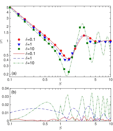
FIG. 2. (Color online) (a) The amplitude of the average pres-sure at the oscillating plate when A = 1: comparison be-tween the results of the LBE for hard-sphere molecules (lines) and the Shakhov kinetic model (symbols, adopted from Fig. 1 in Ref. [12]). Note that here =p⇡/2KnSandS are equiv-alent to the✓andLdefined in Ref. [12], respectively. (b) The absolute value of the relative di↵erence in|p¯(0)|between the LBE for the hard-sphere and Maxwellian molecules.

Similarly, the physical space x and y is divided into Nx⇥Nynonuniform cells, with most of the points located

near the cavity walls [23]:

x=(10 15sx+ 6s2x)sx3, sx= (0,1,· · ·, Nx)

Nx

,

y=(10 15sy+ 6s2y)sy3A, sy= (0,1,· · ·, Ny)

2Ny .

(29)

We chooseNx= 50, andNy= 50 when the cavity aspect

ratio A 1 and Ny = 70 whenA = 2. The numerical

method has been proven accurate [21, 23], in a manner that doubling the number of discretization points in both physical and velocity spaces produces relative di↵erences in macroscopic quantities (such as the amplitude of the average pressure) less than 0.5%.

To demonstrate the accuracy of our numerical method, we consider the sound propagation between two parallel plates (i.e. A=1), and compare the numerical results of the LBE for hard-sphere molecules with those [12] of the Shakhov kinetic model equation [22], in Fig. 2(a). In the numerical simulation, the termvy@h/@yin Eq. (12) is

dropped. When =p⇡/2KnS= 0.1 and 1, the physical space 0 x 1 is divided into 50 nonuniform cells ac-cording to Eq. (29), whilevxis represented by 96

-4 -2 0 2 4 -1

-0.5 0 0.5 1

(b)

-0.01 -0.1

-0.5 -1 -2 -0.6 -0.4 -0.2 0 0.2 0.4 0.6

vx

-0.1 -0.5

-1 -2 -0.06 -0.04 -0.02 0 0.02 0.04

vx

-4 -2 0 2 4

0 0.5 1 1.5

(c)

-0.001 -0.01 -0.1 -0.5 -1 -2 -6 -4 -2 0

-4 -2 0 2 4

-6 -4 -2 0

(a)

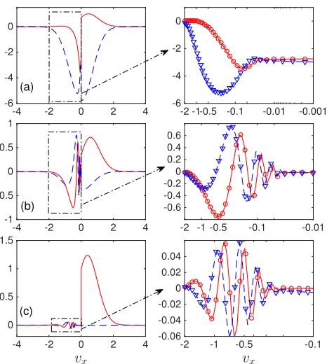
FIG. 3. (Color online) The marginal perturbed distribution function at the oscillating plate,RRh(x= 0,v)dvydvz, when

A=1,Kn= 5p⇡, and the Strouhal number is (a)S= 0.1, (b)S = 1, and (c)S = 10. Large discontinuities and rapid oscillations nearvx= 0 can be clearly seen. Solid lines (or cir-cles) and dashed lines (or triangles) show the real and imag-inary parts of the distribution function, respectively, when

Nv = 192 (or 96). Note that following the rescaling of the perturbed distribution function in Eq. (11),|h/feq|is not nec-essary far less than unitary.

numbers are large. When = 10, the physical space is divided into 150 nonuniform cells, andvx is discretized

by 48 nonuniform points. The comparison in Fig. 2(a) shows that our method has good accuracy.

We have also solved the LBE for Maxwellian molecules, and found that the di↵erence to that of the hard-spheres molecules is very small. For instance, the relative di↵ er-ence in the amplitude of the average gas pressure exerted on the oscillating plate, over a wide range ofSandKnS, is within 4%, see Fig. 2(b). This means that the influence of the intermolecular potential is negligible; hence in the following paper, the LBE for the hard-sphere molecules is used.

It is worthy mentioning that at large values of Kn andS, perturbed distribution functions near cavity walls not only have large discontinuities at vx = 0, but also

oscillate rapidly asvxchanges, see the marginal

distribu-tion funcdistribu-tion in Fig. 3, where the distribudistribu-tion funcdistribu-tion becomes more and more complicated when S increases. This poses a great challenge to the numerical simulation. To reduce the computational cost, Kalempa and Sharipov first introduced additional distribution functions to cast

the three-dimensional molecular velocity space to one-dimensional, and then they split the solution into two parts: the most oscillatory part of the solution is ob-tained analytically [12, 27], while the less oscillatory part is solved numerically, by using a large number of uni-formly discretized velocities. This method, however, may not work in the two-dimensional cavity flow due to the huge computational cost. Alternatively, on noticing that large discontinuities and rapid variations in distribution functions occur nearvx= 0 for the one-dimensional flow

and vx, vy = 0 for the two-dimensional flow, we adopt

the nonuniform discrete velocities, given by Eq. (28), to tackle this problem. The numerical example in Fig. 3 shows that 96 nonuniform discrete velocities in the vx

direction can well capture the oscillatory behavior in the distribution function; as a matter of fact, macroscopic flow quantities such as the average gas pressure do not change (up to the fourth decimal) when increasing the number of discrete velocities fromNv= 96 to 192.

IV. NUMERICAL RESULTS

Now we employ the numerical simulation to investigate the behavior of the average gas pressure and sound speed in the free-molecular, transition, and slip flow regimes, over the whole range of the Strouhal number and a wide range of the cavity aspect ratio.

A. The average gas pressure

x

0 0.2 0.4 0.6 0.8 1

|

¯

p

|

0.2 0.4 0.6 0.8 1 1.2 1.4 1.6 1.8 2

(a)

x

0 0.2 0.4 0.6 0.8 1

Phase

-2.5 -2 -1.5 -1 -0.5 0

x

0 0.2 0.4 0.6 0.8 1

|

¯

p

|

0 0.2 0.4 0.6 0.8 1 1.2 1.4 1.6 1.8 2

(b)

x

0 0.2 0.4 0.6 0.8 1

Phase

-3 -2 -1 0

x

0 0.2 0.4 0.6 0.8 1

|

¯

p

|

0 0.2 0.4 0.6 0.8 1 1.2

(c)

x

0 0.2 0.4 0.6 0.8 1

Phase

-6 -4 -2 0

FIG. 4. (Color online) The amplitude and phase of the average pressure in the free-molecular flow regime with 1/Kn = 0, when the Strouhal number is (a)S= 1.5, (b)S= 3, and (c)S= 9. Along the direction of the arrow, the cavity aspect ratios are 0.125, 0.25, 0.5, 1, 2, and infinity, respectively. In the inset of (c), the phases of the average pressure for di↵erent aspect ratios are nearly indistinguishable, so only the phase forA=1is shown.

value zero, indicating that the high oscillation frequency limit has not been fully reached. From the three insets in Fig. 4 we can see that the phase of the average pressure is not a linear function ofx in the whole domain, which means that the phase speed of the sound wave varies by location.

Figure 5 depicts the average pressure on the oscillat-ing plates, as a function of the Strouhal numberS, at six di↵erent cavity aspect ratios. At large values ofA, as the Strouhal number increases, the amplitude of the average pressure first decreases, then oscillates several times, and finally approaches to a constant value given by Eq. (26) when the oscillation frequency is high. As the aspect ratio decreases, the oscillatory behavior of the average pressure, as a function ofS, becomes weaker and weaker. When the aspect ratio is small enough, sayA=0.25 and 0.125, the oscillatory behavior is completely eliminated. In this case, the increase of the Strouhal number leads to the decrease of the amplitude of the average pressure; and the smaller the value of aspect ratio A, the slower the decrease. The behavior of the phase of the average

pressure as a function of the Strouhal number is, how-ever, in the reverse direction to the amplitude of the av-erage pressure. That is, while the amplitude decreases (or increases) with increasing S, the phase increases (or decreases), which approaches zero when the oscillation frequency is high.

In the one-dimensional geometry (corresponding to A being infinity), the oscillatory behavior of the aver-age pressure as the function of S can be explained by the sound interference [18, 21]. In the free-molecular flow regime, the binary collision is negligible. Using the method of characteristics, Eq. (12) is rewritten as

iSh+⇠@h

@s = 0, ⇠= q

v2

x+vy2, (30)

S

0 1 2 3 4 5 6 7 8 9 10

|

¯

p

|

0 0.5 1 1.5 2 2.5

(a)

S

0 1 2 3 4 5 6 7 8 9 10

Phase

-1.5 -1 -0.5 0 0.5

(b)

FIG. 5. (Color online) The amplitude (a) and phase (b) of the average pressure at the oscillating plate in the free-molecular flow regime with 1/Kn= 0. Along the direction of the arrow, the cavity aspect ratios are 0.125, 0.25, 0.5, 1, 2, and infinity, respectively.

left plate atx= 0, hitting the right plate atx= 1, then being reflected and finally returning to the point from which they left, see type I interference in Fig. 1. The dis-tance gas molecules have traveled is about 2. Therefore, at the resonance frequency

Sr,1'm1⇡, m1= 0,1,2,· · ·, (31) the two distribution functions corresponding to molecules moving leftwards and rightwards have the same phase, so that the gas pressure exerting on the oscillating plate is maximum; similarly, at the anti-resonance frequency

Sa,1' (2n1+ 1)

2 ⇡, n1= 0,1,2,· · ·, (32) the gas pressure on the oscillating plate is minimum.

The above two equations can roughly explain the first anti-resonance (S = 1.5 ' ⇡/2) and resonance (S = 3.2 ' ⇡) frequencies in Fig. 5, when the cavity aspect ratioAis infinity. It can be even applied to the cases of A= 2 and 1.

However, Eqs. (31) and (32) derived from the type I interference has noting to do with the cavity aspect ra-tio and can not explain the behavior of average pressure

S

0 1 2 3 4 5 6 7 8 9 10

|

¯

p

|

0 0.5 1 1.5 2 2.5

(a)

S

0 1 2 3 4 5 6 7 8 9 10

Phase

-1 -0.5 0 0.5

1 (b)

FIG. 6. (Color online) The amplitude (a) and phase (b) of the average pressure at the oscillating plate whenKn= 0.1. Along the direction of the arrow, the cavity aspect ratios are 0.125, 0.25, 0.5, 1, 2, and infinity, respectively.

when A is small, say A = 0.25 and 0.125. This is be-cause whenAis small, gas molecules reflected by the left plate has very small chances of hitting the right plate but are more likely to hit the top and bottom plates, a scenario where the type II interference becomes dom-inant, see Fig. 1. Consider molecules leaving the left plate with velocities nearly parallel to the left plate, hit-ting the top (or bottom) plates, then being reflected and hitting the bottom (or top) plate, and finally returning to the point from which they left. The distance they have traveled is about 2A. Therefore, the pressure on the os-cillating plate is maximum (minimum) at the resonance (anti-resonance) frequency:

Sr,2' m2

A⇡,

Sa,2' (2n2+ 1) 2A ⇡,

(33)

wherem2and n2 are non-negative constants.

is around 2⇡, which means that the amplitude of the average pressure decreases with S when S . 2⇡. And sinceS= 2⇡is very close to the high oscillation frequency limit, the amplitude of the average pressure continues to decrease to the asymptotic limit given by Eq. (26) when S further increases. Type II anti-resonance can also be used to explain why the amplitude of the average pressure decrease more slowly at smaller cavity aspect ratios: the smaller the aspect ratioA, the larger the first anti-resonance frequency Sa,2, and therefore the slower the decaying of the amplitude of the average pressure with respect toS.

We then investigate the average pressure on the oscil-lating plate in the transition and slip flow regimes. To this end, we choose two representative Knudsen numbers, Kn= 1 and 0.1. The results ofKn= 0.1 are presented in Fig. 6, while that of Kn = 1 are not shown as they are very close to those in Fig. 5 in the free-molecular flow regime. Comparisons between Figs. 5 and 6 illus-trate that, asKn decreases, the amplitude of the aver-age pressure oscillates more strongly with S when Ais large. This is comprehensible because smallerKn leads to smaller dissipation and hence larger oscillation ampli-tude; in fact, the oscillation is so large than the second anti-resonance can be easily observed in Fig. 6: inter-estingly, we found that the second anti-resonance fre-quency can be predicted perfectly bySa,1in Eq. (32) with n1= 1, when the aspect ratioAis large. We also found that the first anti-resonance and resonance frequency de-creases slightly withKn.

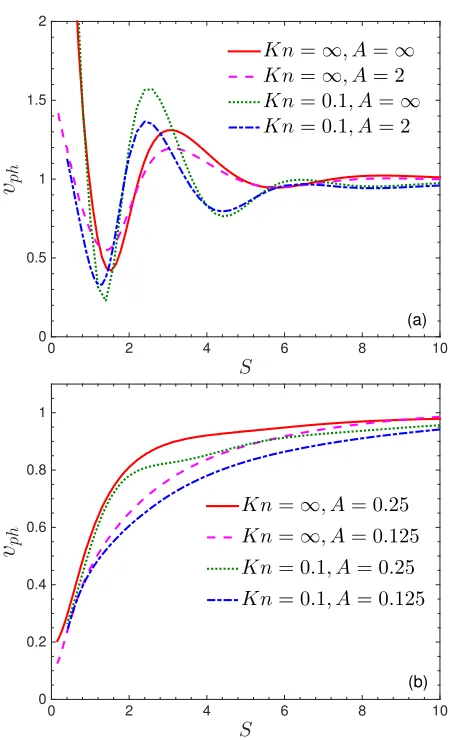
B. The sound speed near the source

We now investigate how the cavity aspect ratio a↵ect the sound speed. Although from the insets in Fig. 4 we see that the phases of the average pressure are not linear functions of x in the whole domain, they vary almost linearly withx close to the sound source, which implies a constant sound speed. Hence we calculate the phase speed of the sound near the sound source as

vph= S

(@ /@x)|x=0

, (34)

where is the phase of the average gas pressure ¯p. Note that the sound speed has been normalized by the most probable speedvm.

It will be interesting to note that, for rarefied gas flows, the di↵erential phase speed defined by Eq. (34) could be negative at some location; for instance, see the variation of the phase near x = 1, at small values of the cavity aspect ratio, in the inset of Fig. 4(a). In this case, the integral phase speed, defined by Eqs. (19) and (21) in Ref. [12], is introduced to calculate the sound speed at the receptor. In the present paper, however, we find that the di↵erential phase speed is always positive near the sound source (see the insets in Fig. 4 near x = 0), so only Eq. (34) is considered.

S

0 2 4 6 8 10

v

0 0.5 1 1.5 2

(a)

Kn=∞, A=∞

Kn=∞, A= 2

Kn= 0.1, A=∞

Kn= 0.1, A= 2

S

0 2 4 6 8 10

v

0 0.2 0.4 0.6 0.8 1

(b)

Kn=∞, A= 0.25

Kn=∞, A= 0.125

Kn= 0_.1_{, A}= 0_.25

Kn= 0.1, A= 0.125

FIG. 7. (Color online) The variation of the sound phase speed near the sound source with the Strouhal number, at large (a) and small (b) values of the cavity aspect ratio.

The analytical solution for the phase speed can also be obtained when KnS 1 andS 1. From Eq. (25) we find that the average pressure near the sound source (whenSx!0) is

¯

p(x) =p1

⇡+

p ⇡

4 iSx'1 iSx. (35)

Thus, the phase of the average pressure near the oscil-lating plate is Sx, and the phase speed near the sound source equals the most probable speed.

increases monotonically withS [Fig. 7(b)], whereas the amplitude of the average pressure decreases monotoni-cally; that is, the phase speed and the amplitude of the average pressure near the sound source are out-of-phase. We also find that, when the values ofKnandSare fixed, smaller value of the cavity aspect ratio leads to smaller value of the sound speed, which is consistent with the discovery in narrow channels [13].

V. CONCLUSIONS

The linearized Boltzmann equation has been solved analytical and numerically to study the sound prop-agation inside rectangular cavities, where one of the cavity walls oscillates and acts as the sound source. It has been found that the damping force (average gas pressure) exerting on the oscillating plate and the sound

speed are significantly a↵ected by the aspect ratio of the cavity. When the aspect ratio is larger than the threshold value of 0.5, the damping force and sound speed oscillate in-phase, as the oscillation frequency increases. However, when the aspect ratio is less than 0.5, the changes of damping force and sound speed are out-of-phase: as the oscillation frequency increases, the damping force decreases, but the sound speed increases. To our knowledge, this exotic behavior of the damping force has not been observed in oscillatory rarefied gas flows before. We attributed this novel phenomenon to a new type of sound interference, occurring in the direction perpendicular to the motion of the oscillating plate. Our proposed simple analytical expressions well predicted the resonance and anti-resonance frequencies.

LW acknowledges the financial support of an ECR In-ternational Exchange Award from the Glasgow Research Partnership in Engineering.

[1] G. Karniadakis, A. Beskok, and N. Aluru, Microflows and Nanoflows: Fundamentals and Simulation(Springer, 2005).

[2] M. GadelHak, “The fluid mechanics of microdevices -the Freeman Scholar lecture,” J. Fluids Eng.121, 5–33 (1999).

[3] J. H. Ferziger and H. G. Kaper,Mathematical Theory of Transport Processes in Gases(North-Holland Publishing Company, Amsterdam, 1972).

[4] C. Cercignani,The Boltzmann Equation and its Applica-tions (Springer-Verlag, New York, 1988).

[5] F. Sharipov, Rarefied Gas Dynamics. Fundamentals for Research and Practice (Wiley-VCH, Berlin, 2016). [6] M. Knudsen, “Die Gesetze der Molekularstr¨omung und

der inneren Reibungsstr¨omung der Gase durch R¨ohren,” Ann. Phys.333, 75–130 (1909).

[7] W. Steckelmacher, “Knudsen flow 75 years on: the cur-rent state of the art for flow of rarefied gases in tubes and systems,” Rep. Prog. Phys.49, 1083–1107 (1999). [8] O. Reynolds, “On certain dimensional properties of

mat-ter in the gaseous state,” Phil. Trans. R. Soc. Lond.170, 727–845 (1879).

[9] J. Nabeth, S. Chigullapalli, and A. A. Alexeenko, “Quantifying the Knudsen force on heated microbeams: A compact model and direct comparison with measure-ments,” Phys. Rev. E83, 066306 (2011).

[10] H. Yamaguchi, M. Rojas-C´ardenas, P. Perrier, I. Graur, and T. Niimi, “Thermal transpiration flow through a sin-gle rectangular channel journal,” J. Fluid Mech. 744, 169–182 (2014).

[11] F. Sharipov and D. Kalempa, “Numerical modelling of the sound propagation through a rarefied gas in a semi-infinite space on the basis of linearized kinetic equation,” J. Acoust. Soc. Am.124, 1993–2001 (2008).

[12] D. Kalempa and F. Sharipov, “Sound propagation through a rarefied gas confined between source and recep-tor at arbitrary Knudsen number and sound frequency,” Phys. Fluids21, 103601 (2009).

[13] N. G. Hadjiconstantinou, “Sound wave propagation in

transition-regime micro- and nanochannels,” Phys. Flu-ids14, 802 (2002).

[14] J. H. Park, P. Bahukudumbi, and A. Beskok, “Rarefac-tion e↵ects on shear driven oscillatory gas flows: A di-rect simulation Monte Carlo study in the entire Knudsen regime,” Phys. Fluids16, 317 (2004).

[15] D. R. Emerson, X. J. Gu, S. K. Stefanov, Y. H. Sun, and R. W. Barber, “Nonplanar oscillatory shear flow: from the continuum to the free-molecular regime,” Phys. Fluids19, 107105 (2007).

[16] T. Doi, “Numerical analysis of oscillatory Couette flow of a rarefied gas on the basis of the linearized Boltzmann equation,” Vacuum84, 734–737 (2009).

[17] X. J. Gu and D. R. Emerson, “Modeling oscillatory flows in the transition regime using a high-order moment method,” Microfluid Nanofluid10, 389–401 (2011). [18] L. Desvillettes and S. Lorenzani, “Sound wave resonance

in micro-electro-mechanical systems devices vibrating at high frequencies according to the kinetic theory of gases,” Phys. Fluids24, 092001 (2012).

[19] D. Kalempa and F. Sharipov, “Sound propagation through a rarefied gas: Influence of the gas-surface in-teraction,” Int. J. Heat Fluid Flow30, 190–199 (2012). [20] Y. W. Yap and J. E. Sader, “Sphere oscillating in a

rar-efied gas,” J. Fluid Mech.794, 109–153 (2016). [21] L. Wu, J. M. Reese, and Y. H. Zhang, “Oscillatory

rar-efied gas flow inside rectangular cavities,” J. Fluid Mech.

748, 350–367 (2014).

[22] E. M. Shakhov, “Approximate kinetic equations in rar-efied gas theory,” Fluid Dynamics3(1), 112–115 (1968). [23] L. Wu, J. M. Reese, and Y. H. Zhang, “Solving the Boltz-mann equation by the fast spectral method: application to microflows,” J. Fluid Mech.746, 53–84 (2014). [24] F. Sharipov and G. Bertoldo, “Numerical solution of

the linearized Boltzmann equation for an arbitrary inter-molecular potential,” J. Comput. Phys.228, 3345–3357 (2009).

coeffi-cients and collision integrals for non-equilibrium gas flow simulations,” Phys. Fluids24, 027101 (2012).

[26] L. Wu, C. White, T. J. Scanlon, J. M. Reese, and Y. H. Zhang, “Deterministic numerical solutions of the Boltz-mann equation using the fast spectral method,” J. Com-put. Phys. (2013).

[27] F. Sharipov and D. Kalempa, “Oscillatory Couette flow at arbitrary oscillation frequency over the whole range of

the Knudsen number,” Microfluid Nanofluid4, 363–374 (2008).