1
Development of an O&M tool for short term decision
making applied to offshore wind farms
Rafael Dawid
1, David McMillan
1, Matthew Revie
1 1University of Strathclyde, Glasgow, UK
Abstract
Every day, wind farm operators make logistical decisions requiring them to efficiently use resources to maximise wind turbine availability. Deciding which turbines to maintain, the order in which they are visited and vessel routing is challenging due to multiple constraints such as weather, failure type and available vessels and technicians. To automate this decision making process, the authors collaborated with a UK offshore wind farm operator to create a tool, which recommends an on-the-day vessel routing strategy, such that costs are minimised while maximising the number of turbines repaired. To demonstrate the tool’s capabilities, a case study is presented and the model’s outputs, which include geographical locations of the turbines to be visited, are shown.
Keywords: offshore wind O&M optimization vessel routing
1. Introduction
In 2015, there was more wind power installed worldwide than any other form of power generation; over 10% of total installed capacity that year was offshore wind power [1]. Effective planning of offshore Operational and Maintenance (O&M) activities, which contribute up to a third of the total cost of energy [2], can increase the availability of turbines and reduce the costs associated with maintenance. As wind farms increase in size and move further offshore, planning offshore maintenance actions is becoming more complex. A recent report by Offshore Renewable Energy Catapult [3] stated that improvement of asset management strategies through the use of decision making tools is a priority for offshore wind O&M.
In reality, time to make decisions on vessel routing and order of repairs is often limited. Furthermore, the difficulty associated with making these decisions increases with the number of turbines which require a maintenance action. The objective is not only to carry out all preventive and corrective actions that are required on the day, but also to do so at the lowest possible cost. High uncertainty associated with planning vessel routing exists, due to weather variability and imperfect fault diagnosis. Efficient automation of the process of vessel routing can contribute significantly to lowering the cost of energy.
1.1 Literature review
2
In terms of research done specifically in the offshore wind domain, it seems that the scientific community only started tackling the Routing and Scheduling Problem of a Maintenance Fleet for Offshore Wind Farms (RSPMFOWF), as introduced by Dai et al. [4], very recently. Dai et al. [4] developed a model for short term planning of vessel routing, which was only tested on up to 8 failed wind turbines. Not all resulting policies generated by the model were optimal due to the complexity of the problem and no limitation was placed on the number of technicians used.Other work in the offshore wind domain includes a paper by Zhang [5], who applied Ant Colony Optimistion (ACO) meta-heuristic technique to solve much larger case studies for offshore vessel routing (up to 28 turbines requiring a maintenance action). The author did not consider the possibility of using the same team of technicians to visit more than one turbine in a day, which in the case studies presented, would result in significant reduction of the number of technicians required. Limiting the number of technicians required on the day can reduce cost of the policy and possibly enable repairing additional turbines, if the problem is constrained by the number of technicians available.
The number of vessels in the case studies for both of the papers discussed above was limited to 2, while most sizeable offshore wind farms have more vessels available at their disposal. Furthermore, the papers mentioned above failed to take into account the transfer time between turbine and vessel. Stålhane et al. [6] offers two solutions to the RSPMFOWF: an arc-flow model producing an exact solution and a path-flow (an arc-flow decomposed using a Dantzig-Wolfe method) heuristic method, which is much more computationally effective, while still producing close to optimal solutions.
Dantzig-Wolfe decomposition method was also applied in a model developed by Irawan et al. [7]. In benchmark tests, their model compared favourably against the algorithm created by Dai et al. [4]. Although the constraints used by both Stålhane et al. [6] and Irawan et al. [7] are more realistic than other papers discussed in this section, the model outputs were not shown or discussed, making it impossible to scrutinise their optimal policies.
All the papers described above would benefit from validation through practical application to a real life problem. Visualisation of the optimal policy in an easily understandable way is a key aspect in transforming the methodologies discussed above into a useful tool that can be used by wind farm operators to plan vessel routing. In this paper, a methodology for solving the RSPMFOWF is presented, which uses a combination of enumeration and a rule based approach. To ensure the model’s applicability in real life, the authors collaborated with an offshore wind farm operator, who validated model’s inputs, assumptions and constraints. The model generates a range of useful outputs which help to visualise the optimal policy.
The problem and the model were described in Section 2. To illustrate the model’s capabilities, a case study is presented, as shown in Section 3. Results are presented in Section 4; Section 5 contains the conclusions and future work.
2. Problem description & model outline
The two key objectives which wind farms operators aim to achieve when planning the vessel routing are:
a) Maximise the number of wind turbines repaired (key performance indicator)
b) Minimise the cost associated with repairing the maximum possible number of turbines
3
Transfer time: it takes a significant amount of time to transfer crew and equipment between a turbine and a vessel
Variable vessel speed: cruise speed in open sea is different to when a vessel is traversing a wind farm
Reusing resources: in certain cases, it may be possible for one crew of technicians to carry out repairs on two different turbines, while still meeting the time constraint
As Irawan et al. [7] pointed out, the most successful exact solutions for the VRPPD split the problem into a master problem, which involves assigning routes to vehicles and one or more sub-problems, wherein routes are created. A similar, two-step approach is applied here.
Let T be a set of turbines which require a maintenance action on the day, while V is a number of vessels available to the operator and v is a given vessel. Matrix M is defined through enumeration, such that each row of M represents a policy (an assignment of vessels to turbines). Since M contains all the possible combinations of assigning vessels to turbines, or not assigning any vessel to a set of turbines, its size is (V+1)^T.
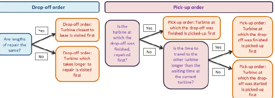
Matrix M is generated in the outer part of the algorithm. The inner part involves splitting up every possible policy (i.e. each row of M) into vectors Fv, which consists of the turbines to be visited by vessel v. The order in which vessel will visit turbines is decided based on a logical algorithm, specific to the length of vector Fv and the classification of lengths of repair of turbines contained in Fv. Length of repair of any turbine can either be classified as type S or L, where S is a repair which takes a short enough time for one crew to carry out two of them in one day. L is a repair which leaves a crew unable to carry out another repair after it has been completed due to the time constraint. An example of the logic used for determining the order in which turbines are visited by a vessel, if it is to visit two turbines, is shown in Figure 1.
[image:3.595.75.521.500.659.2]While the outer layers of the algorithm focus on achieving objectives a) and b) as described above, the inner sub-problem – i.e. the ordering logic algorithm is designed to minimise the time it takes to carry out the maintenance activities. In borderline cases (i.e. when time taken by a policy is close to the time window available on the day) minimising the time taken by a policy is more important than minimising the fuel cost due to distance travelled.
Figure 1. Logic used to determine pick-up and drop-off order for FV length equal to 2 and types
of repair SL, LL or LS.
4
Once the order in which the turbines are visited is determined, it is possible to calculate the estimated time required to carry out a given policy, as shown in Equation 1. Let tv be the time taken by vessel v, B1 is sail time from base to turbine 1, P is time required for transfer of crew and equipment/spares to and from the turbine, D1-2 is the travel time from turbine 1 to turbine 2 and I1 is the idle time due to the vessel waiting for technicians to finish repairs at the first turbine to be picked up.𝑡
𝑣= 𝐵
1+ 𝑃 + 𝐷
1−2+ 𝑃 + 𝐷
2−1+ 𝐼
1+ 𝑃 + 𝐷
1−2+ 𝐼
2+ 𝑃 + 𝐵
2(1)
Policies which contain vectors Fv for which the time calculated in Equation 1 is greater than the time window available on the day are in breach of the model’s time constraint. This and other constraints are shown below:
i) Total time taken by carrying out the policy tv has to be less than specified time window Q
𝑡
𝑣≤ 𝑄 ∀𝑣
ii) Number of technicians required to carry out a policy has to be less than or equal to the number of technicians available
𝑊𝑟𝑒𝑞≤ 𝑊𝑎𝑣𝑎𝑖𝑙
iii) Number of vessels required to carry out a policy Vreq has to be less than or equal to the number of vessels available Vavail
𝑉𝑟𝑒𝑞 ≤ 𝑉𝑎𝑣𝑎𝑖𝑙
iv) The number of technicians on a vessel at any given time Ev cannot exceed the vessel carrying capacity Uv at any time step j
𝑈𝑣
≥ 𝐸
𝑣(𝑗
)∀ 𝑣, 𝑗
If a policy breaches any of the constraints above, it is eliminated from the pool of viable policies. The value Z of all remaining policies is calculated using Equation 2. Let R be the reward of repairing a given turbine, Cr is the cost of repair of a turbine (i.e. cost of spares), Chire is the cost of hiring a given vessel, Cfuel is the cost of fuel used, which is a product of the distance travelled by a given vessel and its fuel consumption.
𝑍 = ∑[𝑅(𝑖) − 𝐶
𝑟(𝑖)]
𝑇𝑖=1
− ∑[𝐶
ℎ𝑖𝑟𝑒(𝑖) + 𝐶
𝑓𝑢𝑒𝑙(𝑖)]
𝑉𝑖=1
(2)
Once Z is calculated for all rows of M, the policy with a maximum value is selected. The following information is displayed to the user:
Map of wind turbine locations and statuses
Vessel routing policy in written and graphical (map) format
Order in which the vessels should visit each turbine
Gantt chart detailing the day’s timetable for each vessel
A 3D value function graph, plotting values of all policies against the two main constraints (time and number of technicians used or time and number of vessels used)
An animation illustrating the order of turbine visits for a vessel requested
5
2.1 Uncertainties
Any activity involving planning future activities will involve a certain degree of uncertainty. When maintaining offshore wind farms, some of the key uncertainties come from:
a) The weather: vessels may be unable to leave base if the wave height limit is exceeded. Furthermore, transfer of technicians and equipment from a vessel onto a turbine may not be possible if the wave height increases during the day. Strong winds may also prevent the crew from carrying out maintenance activities.
b) Human factor: sea sickness or human error may sometimes affect the ability of technicians to carry out the planned activities.
c) Length or type of repair: some failures may be misdiagnosed resulting in repairs taking a longer (or shorter) time or not being successful.
The tool described in this paper focuses purely on the solution of the VRP. However, in practice, operators would be required to make a choice whether to carry out a policy suggested by the model given a forecast with uncertainty. On days, when the forecasted wave height or wind speed are very close to the safe operational limit, or when forecasts have high uncertainty, additional analysis (such as the one described by Browell et al. [8]) should be carried out to determine whether to send vessels out or not.
The key sources of uncertainty described above can impact time and cost of repair and travelling, as well as the number of turbines which have been repaired at the end of the day. It was attempted to reduce the impact of each of those as follows:
Time: the inner sub-problem has been set up so that the time taken by a policy is minimised, rather than cost, although they do go hand in hand most of the time. By doing so, the model ensures that headroom for delays is as large as possible. While the primary objective is to visit as many turbines as possible, doing so in the shortest time possible can be treated as one of the secondary objectives.
Cost: while it is true that a cost of a repair or fuel may exceed the expected value, the authors feel that this has no bearing on the process of planning vessel routing on the day. It is difficult to imagine a situation, wherein a possibility of a repair costing more than expected or the threat of the vessel having to travel a longer distance due to an unexpected circumstance is significantly affecting the decision making, especially since the price of the former would likely have to be paid anyway, while the cost of the latter is relatively low.
Amount of turbines which have been repaired: a probability of successful repair variable has been introduced. If the data from condition monitoring system does not allow pinpointing accurately the root cause of the problem, the model’s user can define a probability of successful repair, which is then multiplied by the reward for visiting this particular turbine.
2.2 Planning horizon
6
2.3 Assumptions
Some of the model’s assumptions are stated below:
a) Vessels start and end their operations at the same maintenance base
b) Technicians are assigned to vessels and are not allowed to be carried by another vessel c) For repairs in the nacelle, time to ascent from sea level (and to descend back down) is
included in the repair time
3. Case study
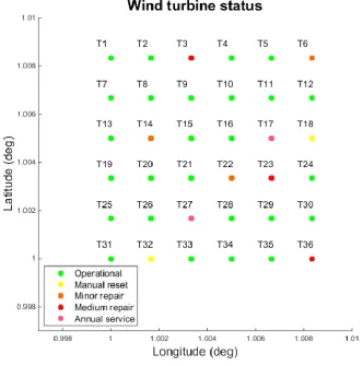
[image:6.595.131.464.327.663.2]Consider the following example motivated by discussions with the offshore wind farm operator. An offshore wind farm consisting of 36 turbines, is located 50km from its maintenance base. On a particular day with good weather and calm sea, 10 out of 36 turbines require a maintenance action. The types of repair range from manual reset and annual service to minor and medium repair. Details of these repairs are outlined in Table 1. A map of this wind farm, including the locations of the turbines which need maintenance actions is shown in Figure 2.
Figure 2. Map of the wind farm detailing the maintenance actions required.
7
Table 1. Classification of failures.Type of failure
Technicians
required
Time
required (h)
Repair
cost
Repair probability
Manual reset
2
2
£0
1
Minor repair
3
4
£3,000
0.9
Medium repair
3
6
£5,000
0.8
Annual service
2
6
£3,000
1
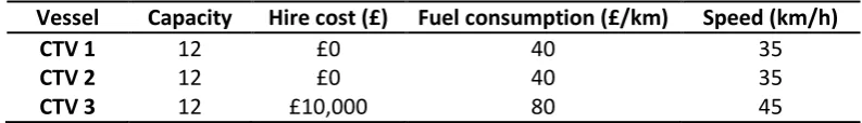
Table 2. Vessel properties.
Vessel
Capacity
Hire cost (£)
Fuel consumption (£/km)
Speed (km/h)
CTV 1
12
£0
40
35
CTV 2
12
£0
40
35
CTV 3
12
£10,000
80
45
3.1 Definition of rewards
As discussed in Section 2.2, the model was designed for on-the-day decision making. However, when defining the reward for repairing a turbine, which is one of the key inputs to the model, looking beyond the one day planning horizon is required. Factors which can affect the reward of repairing a certain turbine are as follows:
a) The revenue generated on the day of the repair, as well as in near future b) Weather forecast
c) Future resource availability and cost
For example consider two turbines which have suffered 2 different types of failure. Turbine 1 requires a simple repair by 2 technicians while turbine 2 requires more complex and costly repair by 3 technicians. If the problem is heavily constrained by the number of technicians available on the day, it’s possible that repairing turbine 1 would be prioritised over turbine 2. However, if wind turbine 2 happens to be on the edge of the wind farm, meaning it produces 20% more power than turbine 1, and supposing that a period of bad weather is expected, meaning that no maintenance can be done in the next week, it may well be worth applying more resources to repair turbine 2, as the revenue generated by it in the next week may be worth it.
The future resource availability can also be a factor. For example, if it is known that the number of resources will increase the following day, or that the cost of using additional resources is set to decrease, it may be beneficial to delay carrying out some of the more complex repairs until the next day, depending on value of the energy that would be generated in the meantime.
The above discussion shows that defining a reward of repairing a certain wind turbine can be a complex procedure. The methodology described by Dawid et al. [10] can be applied in order to calculate the reward of repairing a given turbine, while taking into account the future revenue, weather forecast and expected resource cost and availability.
[image:7.595.98.495.225.282.2]8
4. Results
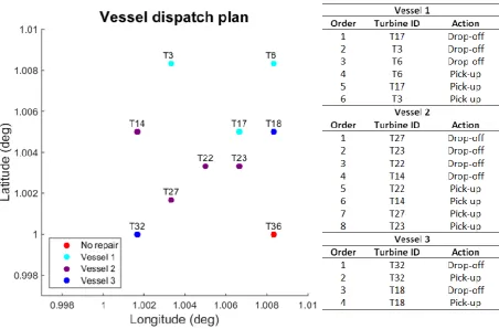
The model described above was implemented in MATLAB and was run on a computer with an i7 3.4GHz processor and 8GB RAM; final result was displayed to the user in 474 seconds. The policy recommended by the model is shown in Figure 3.
Repairing all 10 turbines on that day would require 24 technicians (if the two type S repairs are carried out by the same crew). However, the number of available technicians was only 21; as a result, only 9 out of 10 turbines could have been repaired. T36 was not repaired due to the fact that it required the most costly type of repair and it was located the furthest away from maintenance base of all turbines (the base was located in NW direction).
The algorithm encourages efficient use of technicians by using one team of technicians can carry out repairs at two turbines on the same day. Prioritising such solutions not only enables repairing more turbines, but also uses up less of the vessel capacity, which may mean that fewer vessels are needed to carry out repairs. As turbines T18 and T32 were the only ‘type S’ repairs required on the day, they were serviced using the same vessel (and hence the same team of technicians). This was done using vessel 3, which is the quickest of all vessels. The reason for the model assigning the “simplest” route to vessel 3 was its higher fuel consumption.
[image:8.595.75.528.148.446.2]Vessels 1 and 2 are each assigned a cluster of turbines which are located close to each other, which minimises both the fuel cost and the time spent travelling between turbines. It is also worth noting that the first two turbines visited by vessels 1 and 2 are the longest (6 hour) repairs, making the best use of the limited time window. Although just 2 vessels would have been enough to carry all the technicians that day, there would not have been enough time to carry out repairs with vessels 1 and 2
9
only. Hence vessel 3 had to be hired out at an extra cost to ensure the maximum number of turbines was repaired.5. Conclusions
The model described here allows effective planning of resources by automating the process of logistical decision making of maintenance actions for offshore wind farms. Maintenance decisions are still predominantly made without the assistance of mathematical models and given the large number of possible policies, operators may miss a policy that allows repairing an additional wind turbine. This would be particularly important if a period of rough sea is expected in near future, meaning no possible repairs for a certain period of time.
Furthermore, automating the decision making process by using the model described here would likely save time and resources, while extending the effective repair window. The user-friendly outputs produced by the model, help to visualise the policy, making it appealing to the practitioners. The model’s use is not restricted to CTVs; the use of helicopters, which are becoming more widespread, can also be captured by the model.
Future work could focus on both practical and theoretical developments. Firstly, the authors aim to apply the model to a real life case study, as a part of the validation process. This could be realised through a blind case study, in which the information available to the operator at the start of the day is used as an input to the model. The outputs would then be compared to the decision made by the operators to see whether the model proposed a policy that is viable and whether it would enable repairing more turbines, or repairing the same amount at a lower cost.
10
6. References
[1] G. Corbetta, A. Mbistroba, and A. Ho, “Wind in power 2015 European statistics”, The European Wind Energy Association, 2016.
[2] M. Scheu, D. Matha, M. Hofmann, and M. Muskulus, “Maintenance strategies for large offshore wind farms,” Energy Procedia, vol. 24, no. January, pp. 281–288, 2012.
[3] M. Newman, “Operations and maintenance in offshore wind: key issues for 2015/16”, Offshore Renewable Energy Catapult, 2015.
[4] L. Dai, M. Stålhane, and I. B. Utne, “Routing and Scheduling of Maintenance Fleet for Offshore Wind Farms,” Wind Eng., vol. 39, no. 1, pp. 15–30, 2015.
[5] Z. Zhang, “Scheduling and Routing Optimization of Maintenance Fleet for Offshore Wind Farms using Duo-ACO,” Adv. Mater. Res., vol. 1039, pp. 294–301, 2014.
[6] M. Stålhane, L. M. Hvattum, and V. Skaar, “Optimization of Routing and Scheduling of Vessels to Perform Maintenance at Offshore Wind Farms,” Energy Procedia, vol. 80, no. 1876, pp. 92–99, 2015.
[7] C. A. Irawan and D. Ouelhadj, “Optimisation of maintenance routing and scheduling for offshore wind farms,” Eur. J. Oper. Res., vol. 256, no. 1, pp. 76–89, 2015.
[8] J. Browell, I. Dinwoodie, and D. McMillan, “Forecasting for Day-ahead Offshore Maintenance Scheduling under Uncertainty,” in ESREL, 2016.
[9] M. Antrobus and R. Sykes, “Industry challenges report: Novel vessels and equipment”, Logistic Efficiencies And Naval architecture for Wind Installations with Novel Developments (LEANWIND), 2014.