Three-dimensional temperature field
measurement of flame using a single light field
camera
Jun Sun,1 Chuanlong Xu,1,* Biao Zhang,1 Md. Moinul Hossain,2 Shimin Wang,1 Hong Qi3 and Heping Tan3
1Key Laboratory of Energy Thermal Conversion and Control of Ministry of Education, School of Energy and
Environment, Southeast University, Nanjing, 210096, PR China
2Department of Chemical and Process Engineering, University of Strathclyde, Glasgow, G1 1XJ, UK 3School of Energy Science and Engineering, Harbin Institute of Technology, 92, West Dazhi Street, Harbin 150001,
PR China *[email protected]
Abstract: Compared with conventional camera, the light field camera takes the advantage of being capable of recording the direction and intensity information of each ray projected onto the CCD (charge couple device) sensor simultaneously. In this paper, a novel method is proposed for reconstructing three-dimensional (3-D) temperature field of a flame based on a single light field camera. A radiative imaging of a single light field camera is also modeled for the flame. In this model, the principal ray represents the beam projected onto the pixel of the CCD sensor. The radiation direction of the ray from the flame outside the camera is obtained according to thin lens equation based on geometrical optics. The intensities of the principal rays recorded by the pixels on the CCD sensor are mathematically modeled based on radiative transfer equation. The temperature distribution of the flame is then reconstructed by solving the mathematical model through the use of least square QR-factorization algorithm (LSQR). The numerical simulations and experiments are carried out to investigate the validity of the proposed method. The results presented in this study show that the proposed method is capable of reconstructing the 3-D temperature field of a flame.
2015 Optical Society of America
OCIS codes: (110.0110) Imaging systems; (120.0120) Instrumentation, measurement, and me-trology.
References and links
1. P. Norbert. Combustion Theory (2000).
2. J. Ballester, and T. García-Armingol. “Diagnostic techniques for the monitoring and control of practical flames,” Prog. Energ. Combust. 36(4), 375-411 (2010).
3. T. Lee, W. G.Bessler, H. Kronemayer, C. Schulz, and J. B. Jeffries. “Quantitative temperature measurements in high-pressure flames with multiline NO-LIF thermometry,” Appl. Optics. 44(31), 6718-6728 (2005). 4. J. Doi, and S. Sato. “Three-dimensional modeling of the instantaneous temperature distribution in a turbulent
flame using a multidirectional interferometer,”Opt. Eng. 46(1), 015601-1-015601-7 (2007).
5. H. N. Yang, B. Yang, X. S. CAI, C. Hecht, T. Dreier, & C. Schulz. “Three-dimensional (3-D) temperature measurement in a low pressure flame reactor using multiplexed tunable diode laser absorption spectroscopy (TDLAS),” Laser. Eng. 31, 285-297 (2015).
6. M. M. Hossain, G. Lu, D. Sun, and Y. Yan. “Three-dimensional reconstruction of flame temperature and emissivity distribution using optical tomographic and two-color pyrometric techniques,” Meas. Sci. Technol. 24(7), 1-10 (2013).
8. M. M. Hossain, G. Lu, and Y. Yan. “Optical fiber imaging based tomographic reconstruction of burner flames,” IEEE T. Instrum. Meas. 61(5), 1417 – 1425 (2012).
9. H. Zhou. The Principle and Technology of Visualization from Flames in Boiler (2005).
10. H. Zhou, X. Lou, and Y. Deng. “Measurement method of three-dimensional combustion temperature distribution in utility furnaces based on image processing radiative,” in Proceedings of the Chinese Society for Electrical Engineering, (1997), pp. 1-4.
11. W. Li, C. Lou, Y. Sun, and H. Zhou. “Estimation of radiative properties and temperature distributions in coal-fired boiler furnaces by a portable image processing system,” Exp. Therm. Fluid SCI. 35(2), 416-421 (2011).
12. X. Wang, Z. Wu, Z. Zhou, Y. Wang, and W. Wu. “Temperature field reconstruction of combustion flame based on high dynamic range images,” Opt. Eng. 52(4), 043601-01-043601-10 (2013).
13. C. Lou, Y. Sun, and H. Zhou. “Measurement of temperature and soot concentration in a diffusion flame by image processing,” J. Eng. Thermophys. 31(9), 1595-1598 (2010).
14. A. Gershun, “The light field,” J. Math. Phys. Camb. 18(1), 51-151 (1939).
15. E. H. Adelson, and J. Y. A.Wang. “Single lens stereo with a plenoptic camera,” IEEE T. Pattern Anal. 14(2), 99-106 (1992).
16. R. Ng, M. Levoy, M. Brédif, G. Duval, M. Horowitz, and P. Hanrahan. “Light field photography with a hand-held plenoptic camera,” Computer Science Technical Report CSTR of Stanford University, 1-11 (2005). 17. T. Georgiev, and A. Lumsdaine. “Focused plenoptic camera and rendering,” J. Electron. Imaging 19(2),
021106-1-021106-11 (2010).
18. J. T. Bolan, K. C. Johnson, and Thurow, B. S. “Preliminary investigation of three-dimensional flame measurements with a plenoptic camera,” In Proceedings of 30th AIAA Aerodynamic Measurement Technology and Ground Testing Conference (AIAA , 2014), pp. 1-12.
19. L. Ruan, H. Qi, S. Wang, H. Zhao, B. Li. L. Ruan. “Arbitrary directional radiative intensity by source six flux method in cylindrical coordinate,” Chinese J. Comput. Phys. 26(3), 437-443 (2009).
20. A. Lumsdaine, and T. Georgiev. “The focused plenoptic camera,” In Proceedings of IEEE Conference on Computational Photography (ICCP)( IEEE 2009), pp. 1-8.
21. P. Lin. New Computation Methods for Geometrical Optics (Springer, 2014).
22. A. Fusiello “Elements of geometric computer vision,” http://homepages. inf. ed. ac. uk/ rbf/ CVonline/ LOCAL_COPIES /FUSIELLO4/ tutorial.
23. Q. Huang, F. Wang, J. Yan, and Y. Chi. “Determination of soot volume fraction and temperature distribution in ethylene/air non-premixed flame based on back-projection algorithm,” J. Combust. Sci. Technol. 15(3), 209-213 (2009).
24. J. Felske, and C. Tien. “Calculation of the emissivity of luminous flames,” Combust. Sci. Technol. 7(1), 25-31 (1973).
25. C. Paige, and M. Saunders. “LSQR: An algorithm for sparse linear equations and sparse least squares,” ACM T. Math. Software 8(1), 43-71 (1982).
26. M. Saffaripour, A. Veshkini, M. Kholghy, M. J. Thomson. “Experimental investigation and detailed modeling of soot aggregate formation and size distribution in laminar co-flow diffusion flames of Jet A-1, a synthetic kerosene, and n-decane,” Combust. Flame 161(3), 848-863 (2014).
27. S. R. Turns. An Introduction to Combustion (1996).
28. I. Ayrancı, V. Rodolphe, S. Nevin, A. Frédéric, and E. Dany. “Determination of soot temperature, volume fraction and refractive index from flame emission spectrometry,” J. Quant. Spectrosc. Ra. 104(2), 266-276 (2007).
1. Introduction
flame for in-depth understanding of the combustion mechanism, and subsequent optimization of combustion process and pollutant formation process.
Various measurement techniques have been reported over the past decades for the 3-D temperature field measurement of flame, for instance laser-based diagnostics [3-5] and radiative imaging techniques [6-13]. Laser-based techniques are active measurement methods, which employ the measured scattering, absorption and fluorescent signals caused by the laser crossing the flame to derive the temperature [3-5]. For example, the fluorescence of the species (e.g., NO) excited with a laser is utilized in laser-induced fluorescence (LIF) thermometry. However, due to the complexity and high cost of the laser-based diagnostic systems, these techniques are generally unsuitable for the applications in hostile industrial environments. The limited power of lasers also limits the applicability of laser-based diagnostics. In radiative imaging technique, the visible radiation information is usually applied to measure the temperature fields of flames. This technique doesn’t require imposing external signal and hence they are simple in system setup compared with laser-based diagnostic system. For example, Hossain et al. [6-8] developed optical tomographic algorithms incorporating logical filtered back-projection and simultaneous algebraic reconstruction techniques to reconstruct the grey-level intensities of flame sections. The flame temperature distribution is obtained from the reconstructed grey-level intensities of the image based on the two color method. Zhou et al. [9-11] proposed a radiative imaging model which relates flame image with the temperature distribution based on conventional CCD camera. The 3-D flame temperature is then reconstructed using a Tikhonov regularization method to solve the model. Wang et al. [12] used HDR (high dynamic range) cameras to avoid the loss of information caused by overexposure or underexposure. The flame radiant existence field is reconstructed using the flame image, and temperature field is further calculated via the lookup table between radiant existence and temperature. These researches proved that the radiative imaging technique is efficient for the 3-D temperature field reconstruction in large scale flames. However, up to date the conventional cameras are used for these radiative imaging techniques to record the radiation intensity where the direction of each ray cannot be recorded simultaneously. So the multi-cameras are needed in radiative imaging system for the measurement of flame temperature field. This leads to some issues such as high degree of coupling and synchronization of the multi-cameras, making the operation and mounting of the system costly and inconvenient. A single camera system has also been employed for the radiative imaging technique [13] to reconstruct the 3-D temperature field. In this model, the beam of rays detected by each pixel is regarded as the principal ray for simplification. However, the simplification is based on the fact that the distance between the camera and the flame is far enough. The farther distance will result in the smaller image of the flame with certain size. The smaller image implies that the pixels of the CCD sensor are not employed to capture the flame image at the utmost extent.
focused light field camera. Rather than placing the CCD sensor at the distance of the focal length of the microlenses, it is placed at a distance unequal to the focal length. In this case, the spatial and direction samplings are traded off more reasonably to render high resolution images. The radiation from flame in combustion apparatus is also seen as light filed, and so a single light field camera can capture the radiation of flame with a single exposure. Due to the high direction sampling of light field camera, the far distance is not necessary for 3-D temperature measurement if a single light field camera is used. In addition, the principal ray in light field camera is more representative for the beam compared to conventional camera duo to the smaller cone angle of this beam. Combined with suitable radiative imaging model and inverse reconstruction algorithms, one single light field camera may measure the 3-D temperature field of the flame. Up to date, the research on the application of light field camera in the 3-D flame diagnostics is very limited. For instance, Jeffrey et al. [18] preliminary investigated the 3-D measurement of flames with a light field camera using image refocusing, 3-D deconvolution and tomographic reconstruction techniques. However, feasible methods are not proposed to reconstruct the 3-D temperature field of the flame.
This paper aims to present a novel method for reconstructing 3-D temperature field of a flame based on a single focused light field camera. The principal ray projected onto the pixel of the CCD sensor is traced in the radiative imaging model. Further, the intensities of the principal rays recorded by the pixels on the CCD sensor are mathematically modeled based on radiative transfer equations [19]. The 3-D temperature field of a flame can then be reconstructed by solving the mathematical model through use of least square QR-factorization algorithm (LSQR). Experiments and simulations are performed on the co-flow burner of the ethylene flames to evaluate the method. Finally the results obtained from the experiments and simulations are presented and analyzed in details.
2. Measurement principle
2.1 Radiative imaging model
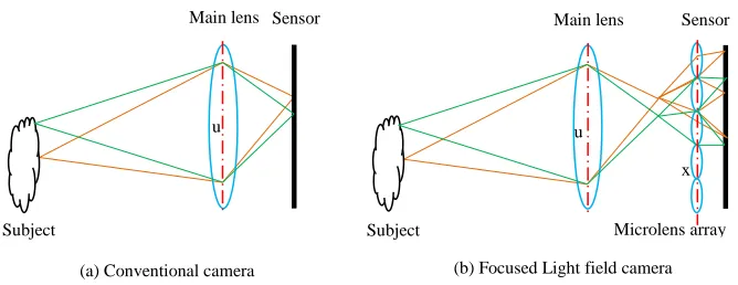
Fig. 1. Schematic diagram of sampling of the rays with conventional camera and focused light field camera
In light field camera, the focal plane is the conjugate plane of the sensor plane. However, the radiation of particles in whole flame contributes to the final image. So as shown in Fig. 2, the focal plane of the light field camera applied to capturing translucent medium is called virtual focal plane, and the points on the virtual focal plane are called virtual source points. The virtual image plane is the conjugate plane of the virtual focal plane for the main lens. As a consequence, the intensity and the direction information of the flame radiation filed is simultaneously recorded by the light field camera.
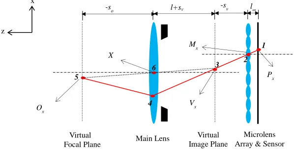
Fig. 2. Schematic diagram of radiative imaging model for flames using a single light field camera
Cone angle (e.g. θ or ψ in Fig. 2) is defined as the apex angle of the cone of the beam projected on the pixel of CCD sensor. All radiations around the virtual source point within the cone angle contribute to the radiation intensity detected by the pixel. The smaller cone angle means the better representative for the direction of the beam projected onto the pixel on sensor [9, 10]. Figure 3 shows the comparison of the cone angles of the beam detected by the pixels (in a column) of the conventional camera and the light field camera. The diameter of the main lens pupil of the cameras is 3 mm, and the distance between the principal plane of the main lensand the flame (central plane of the flame) is set to 400 mm. The resolutions of the camera sensors are fixed to 900 (H) ×900 (V). From Fig. 3, it can be seen that the cone angle (θ) of the light field camera is much smaller than that of the conventional camera. This is because that the beam of rays from the virtual source point is divided into several beams by the microlenses. So the gray level of the pixel in the light field camera is more representative for
Main lens Sensor
u
Subject
(a) Conventional camera
Main lens Sensor
Microlens array u
x
Subject
(b) Focused Light field camera
Main lens
Sen-sor Flam
e
M
icr
o
le
n
s a
rr
ay
V
ir
tu
al
i
m
ag
e
p
la
n
e
V
ir
tu
al
f
o
ca
l
p
la
n
e
[image:5.610.181.431.348.505.2]the radiation information at that direction than that of the conventional camera.
Fig. 3. Comparision of cone angles of the beam detected by the pixels (in a column) on sensor of conventional camera and light field camera
Since the cone angle (θ) of the beam detected by the pixel is so small (<0.015°) in the light field camera, the principal ray (marked as red in Fig. 2) which crosses through the pixel and the center of its corresponding microlens is used to represent the beam. This ray is called the corresponding ray of the pixel in this study. The corresponding ray must be traced from the sensor pixel to the flame to obtain the direction of the flame radiation outside the camera. In this paper, pinhole camera model is applied to trace the rays [21, 22]. In camera coordinate system, the principal point of the main lens is taken from origin and x and y axes are parallel to sensor plane, and z axis is normal to sensor plane. As shown in Fig. 4, the center of the pixel (point 1) and virtual image (point 3) is conjugated for the corresponding microlens whose center is point 2. Point 3 and virtual source point 5 is conjugated for main lens whose center is point 6. So the coordinate (Vx, Vy) of point 3 can be derived by,
1
1
1
-
=
m v m
l
s
f
(1)
-= =
-
-y y
x x m
x x y y v
P M
P M l
V M V M s (2) where (Px, Py) is the coordinate of point 1 and (Mx, My) is the coordinate of point 2, lm is the distance between the microlens array and the sensor plane, –sv is the distance between the
0 200 400 600 800
0.3610 0.3615 0.3620 0.3625 0.3630 0.3635
Con
e a
ng
le
(
)
Pixel
0 200 400 600 800
0.01392 0.01394 0.01396 0.01398 0.01400 0.01402 0.01404 0.01406
Con
e a
ng
le
(
)
Pixel
(a) Conventional camera
microlens array and the virtual image plane, fm is the focal length of the microlens. The coordinate (Ox, Oy) of point 5 is then calculated by,
1
-
1
=
1
+
v ol
s
s
f
(3)-- +
= =
-
-y
x v
x y o
V Y
V X l s
[image:7.610.145.444.266.425.2]O X O Y s (4) where (X,Y) is the coordinate of point 6, l is the distance between the main lens and the microlens array, l+sv is the distance between the main lens and the virtual focal plane, f is the focal length of the main lens, –so is the distance between the main lens and the virtual focal plane. The corresponding ray of the pixel will intersect the principal plane of the main lens at point 4. The direction of the flame radiation outside the camera is obtained by connecting point 4 and point 5 as shown in Fig. 4.
Fig. 4. Schematic diagram of ray tracing in focused light field camera
2.2 Mathematical model for flame temperature
The intensity detected by the pixel is regarded as the intensity of the corresponding ray, which can be calculated using radiative transfer equation of the flame [23]. The intensity of the ray along the path s can then be expressed by,
4
-
( , )
4
bdI
k I
I
I
s s d
ds
(5)
where Iλ is the monochromatic intensity of blackbody radiation, W/(m3∙sr). s is the length along the direction of the ray. Φ(s’, s) is the scattering phase function between incoming direction s’ and scattering direction s. Ω is the solid angle in direction s’. kλ, βλ, and σλ are the monochromatic emission, absorption and scattering coefficients, respectively, (m-1). According to [24], soot particles in flame are both absorbing and scattering, and yet the scattering cross-section is much smaller than the absorption cross-section. For simplification, the scattering of the participating medium is ignored and absorption is only taken into consideration in this paper. Then by employing optical thickness τ which is the integral of absorption coefficient within the length s, equation (5) can be discretized as follows
Mx
Main Lens
X
Ox Vx
-so l+sv
Microlens Array & Sensor
Px -sv lm
Virtual Image Plane Virtual
Focal Plane x
z
1
2 3
4 5
1
1 1
(1 exp(1
))
(exp(
) exp(
))
n n n
n b n n j j b i
i j i j i
I
I
I
where Inλ is the final radiation intensity of the ray crossing through the flame. Ibλ and τ are the monochromatic intensity of blackbody radiation and optical thickness of the voxel which the ray passes through respectively and n is the number of the voxel. So a linear equation for the corresponding rays is derived and defined as follows,
ccd λ
I A IB
(7) where Iccd is the matrix of the intensity distribution on the CCD sensor, IBλ is the matrix of the all voxels and can be calculated with the monochromatic intensity of blackbody radiation. A is the coefficient matrix related to the optical thickness and will be obtained using Eq. (6) with known absorption coefficient.
2.3 Inverse algorithm
The resolution of the light field camera sensor is usually very high [4384(H)×6576(V)]. So the pixels covered by the flame image are up to 10000 and the radiative transfer equations composing Eq. (7) is enormous. Meanwhile, each corresponding ray of the pixel passes through a small percent of all voxels, and so the coefficients of each equation in system of linear equations (7) are mostly zero. Therefore A in Eq. (7) is a sparse large and ill-conditioned matrix. Least square QR-factorization (LSQR) algorithm finds a solution to the least squares problems [25]. The method is based on the bidiagonalization procedure of Golub and Kahan. It is analytically equivalent to the standard method of conjugate gradients, but purportedly has the best numerical stability when A is ill-conditioned. So in this paper LSQR algorithm is used to solve Eq. (7) and to receive the monochromatic intensity of blackbody radiation Ibλ of each voxel. The temperature T of each voxel is then calculated using Eq. (8) according to Planck’s law.
5
2
/ ln[ / (
1 b1)]
T
c
c
I
(8) where c1 is the first radiation constant, 3.7418×10⁻¹⁶ W∙m2 and c2 is the second radiation constant, 1.4388×10⁻² m∙K. λ is the wavelength of the ray. Note that the direct solution of Eq. (7) using this algorithm may have negative values of Ibλ. So non-negativity constraint must be added during iterations. Specifically, an initial guess Ibλ≥0 is chosen and the update step is replaced by projecting the iteration Ibλ(k) onto the nonnegative orthant.
2.4 Radiation intensity calibration
A pre-calibrated blackbody furnace (LANDCAL R1500T) is utilized to calibrate the radiation intensity of the CCD sensor to convert flame image into the intensity distribution [13]. It is deemed that the sensor receives the whole radiation of the blackbody furnace. So when the temperature of the blackbody furnace is T, the radiation intensity I detected by the sensor is calculated by,
)
1
-)]
/(
(exp[
=
2 5 -1
T
λ
c
π
λ
c
I
(9)is less than 1%. The average gray level is normalized to its maximum value (255) at which the image is approaching saturation. A second order polynomial function is applied to obtain the relationship between the average gray level of Red (R), G (Green) and B (Blue) channels images and the corresponding radiation intensity. The fitted results are shown in Fig. 5. It can be seen that the radiation intensity of R channel is more sensitive to gray level than those of G and B channels. So the output of R channel is selected for the conversion from flame image to the radiation intensity.
Fig. 5. Relationship between the blackbody furnace images and the corresponding radiation intensity
3. Experimental setup
Figure 6 illustrates the schematic diagram of the experimental setup. It is mainly comprised of two parts, i.e. the burner along with essential elements (Pressure reducing valve, pressure gauge, flow meter and needle valve) and the light field camera combined with the application software and computer. During the experiments, the compressed air and ethylene (C2H4) are
supplied from air and fuel cylinders and pass through the pressure reducing valve, pressure gauge, rotameter and needle valve mounted on the different tubes to the burner. The air and ethylene flow rates are controlled by the rotameters.
To create stable flames a co-flow diffusion burner is fabricated in this study and basically it is scaled down of [26]. Figure 7 shows a schematic structure of the co-flow diffusion burner. This burner is comprised of an inner tube and an external tube. The inner tube is for fuel flow while the external one is for air flow. The diameters of the inner and external tubes are 12 mm and 50 mm, respectively. The space between the two tubes has an insert of glass bead with the diameter 3 mm and mesh to minimize the flow non-uniformities. To eliminate the influence of ambient light or light reflected, the burner is placed inside a chamber with the black background.
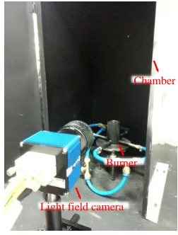
The focused light field camera (R29 of Raytrix, RGB) is placed one side of the flame to capture the flame image, as shown in Fig. 8. The distance between the camera and the flame is set to 400 mm so that the whole flame can be captured. The number of the microlenses of the microlens array is 207×160. The KAI-29050 interline CCD color image sensor of the camera has a resolution of 6576(H)×4384(V). The corresponding wavelengths of R, G and B
channel of the sensor are 610 nm, 530 nm and 460 nm respectively. The application software is used to control the light field camera and store the captured images. The digital output resolution is 8bit using 14bit ADC (Analog to digital converter). The raw image captured by the camera is a Bayer pattern image. In this experiment, the exposure time of the light field
0.0 0.2 0.4 0.6 0.8 1.0 0
1x10⁷
2x10⁷
3x10⁷
4x10⁷
5x10⁷
6x10⁷
R G B R(fitting) G(fitting) B(fitting)
Radiat
ion
Int
ensit
y /
(W/m
3 sr
)
Normalized Gray Level
IB=310.50+8054.26B+2.43B2
IG=-109748.14+2.73
G+9.68
G2
camera (exposure time range 17 μs-60 s) is set to 0.8 ms and found that the captured flame images are not too dark and not saturated.
[image:10.610.149.473.109.250.2]Fig. 6. Schematic diagram of the experimental setup
Fig. 7. Schematic of the co-flow diffusion burner
Fig. 8. Physical implementation of the flame imaging system Ethylene
Computer
Air
Burner Light field camera
Optical table Support Chimney
Chamber Pressure reducing valve
Pressure gauge
Needle valve Rotameter
Pressure reducing valve Pressure gauge
Rotameter
Needle valve
Glass bead 3 Mesh 0.8 50
10 5 5
1
0
0
5
15
50
20
10
6
2
2
2
A A
A-A Fuel
Air Air
Unit: mm
Chamber
Burner
Light field camera
[image:10.610.237.363.470.636.2]
4. Results and discussions
4.1 Simulations
In order to prove the feasibility of the proposed method, a numerical simulation was performed. In this study the simulation results can be served as a basis for further experimental research. A cylindrical flame in a dark environment is captured using the light field camera for the flame simulation. The monochromatic radiation intensity of the blackbody of all voxels IBλ is calculated with known temperature using the Planck’s law. Each corresponding ray of the pixel is traced using the Eqs. (1-4) to determine the direction of flame radiation outside the camera. A is then obtained with known absorption coefficient based on Eq. (6). The intensity distribution Iccd on the CCD sensor is calculated with known IBλ and A using Eq. (7). The intensity distribution Iccd is added with 1% Gaussian noise as measurement errors and then used to reconstruct 3-D temperature field of the flame. Without loss of generality for the proposed method, the parameters of this simulation are not set exactly the same as the experimental parameters.
For this simulation the height and radius of the cylindrical flame are considered 40 mm and 20 mm, respectively. The absorption coefficient of the flame is used 0.5 m-1 and similar coefficient was considered by [19]. The temperature distribution of an axis-symmetrical flame is defined as follows
2 2
( , ) 2600( - 0.04 0.1) (0.004 - ) 800( )
T x r x x r K (9) where x and r denote the axial and radial coordinates of the cylindrical flame, respectively. The flame is divided into voxels in the circumferential direction (NO), radial direction (NR) and
axial direction (NX). The total number of voxels (NO×NR×NX) is (6×6×6) =216 in this
simulation. The distance between the main lens (principal plane) and the microlens array is 180 mm. The distance between the microlens array and the sensor plane is 765μm. The focal length of the main lens is 50 mm. The focal length of each microlens is 567 μm. There are 100×100 microlenses of the microlens array. The diameter of each microlens is 90 μm. The resolution of the camera sensor is 900(H)×900(V). The size of each pixel is 10×10 μm.
Figure 9 shows the simulated intensity (normalized) distribution on CCD sensor plane. This distribution can be seen as a raw image captured by the light field camera. It has the appearance of being a conventional photograph when viewed macroscopically. However, it is composed of many macro pixels when the image is magnified. It is because that the round diaphragm of the main lens confines the rays to a circular area beneath each microlens and hence the flame radiation cannot be detected by the pixels between the circular areas.
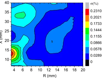
Figure 10 shows the relative error of the reconstructed results. In this figure, the relative error of the ith voxel is defined as
%
100
×
-=
exai exa i est i
i
T
T
T
σ
(10)Fig. 9. Simuated gray level intensity distributions on CCD sensor plane
Fig. 10. Relative error of the reconstructed 3-D temperature field of the simulated flame
4.2 Experiments
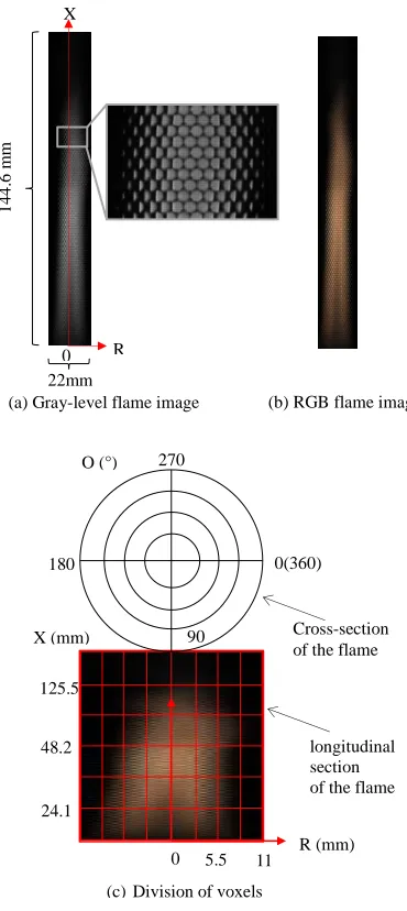
The raw image of the flame with a close-up sub-image is shown in Fig. 11(a). In this experiment the volumetric flow rates of fuel and air are supplied 20.9 mL/s and 0.4 L/s respectively (air to fuel equivalence ratio is 1.37). The image is firstly pre-processed including denoising (removing dark noise of the sensor) and demosaics (obtaining R gray level of each pixel from raw Bayer pattern image). The processed flame image as shown in Fig. 11(b) is then converted into the intensity distribution according to the intensity calibration results.
4 6 8 10 12 14 16 18 20
10 15 20 25 30 35 40
X
(
m
m
)
R (mm)
0 0.0289 0.0578 0.0866 0.1155 0.1444 0.1733 0.2021 0.2310
[image:12.610.212.382.234.364.2]Fig. 11. Flame image captured by the light field camera (a) and (b), and corresponding schematic of division of voxels (c)
The flame is treated here as a cylinder with the height and diameter of 144.6 mm and 22 mm, respectively. To ensure the uniqueness of the least square solution of (7), the number of voxels should equal to the rank of matrix A [25]. So the flame is divided into NO×NR×NX =
4×4×6 (96) voxels for this purpose and Fig. 11(c) shows the schematic division of voxels (not to scale). In this figure, the upper circle denotes the division in O (0°~360°) and R directions over a cross-section of the flame and the rectangle below it denotes the division in X (0~144.6 mm) and R directions (-11~11 mm) over a longitudinal section of the flame. The absorption coefficient of the flame is 0.8 m-1 [23, 24] considered in this experiment.
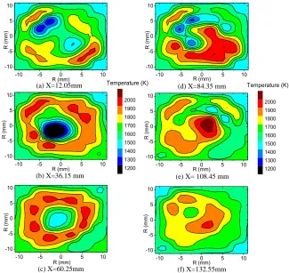
Figure 12 shows the reconstruction of 2-D temperature distribution over the cross-sections of the flame. It can be seen that the temperature of the flame is within the range of 1200K to 2100K and similar ranges were also found by others researchers [13, 28] with same operating
22mm R X
1
4
4
.6
m
m
(a) Gray-level flame image 0
(b) RGB flame image
(c)Division of voxels
R (mm) X (mm)
24.1 48.2 125.5
11 0
O (°)
0(360)
90 180
270
Cross-section of the flame
longitudinal section of the flame
condition. Basically, in diffusion flame the fuel flows along the flame axis diffuses rapidly outward and the air diffuses rapidly inward [27]. Flame surface is defined as a thin zone where the fuel-air equivalence ratio equals unity. Chemical reactions occur in this zone, including the destruction of the fuel molecules and the creation of many species. The reaction zone is annular until the flame tip. The temperature is high in this zone due to the bulk chemical energy release. Away from this zone (outward or inward), the temperature gradually decreases. So theoretically the 2-D temperature distribution over each cross-section of the flame should be annular. The temperature of the annulus in the reaction zone is higher than that of the other zones. With increasing R, the temperature of radial voxels firstly increases and then decreases. From Fig. 12, it can also be seen that 2-D temperature distribution over each cross-section is annular. However, the annuluses are not uniform and symmetrical especially over cross-sections X =84.35 mm and X =108.45 mm. It is because that the flow (i.e. air and ethylene flow) is probably not stable enough and the tube of the burner may be not quite symmetrical.
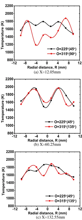
[image:14.610.151.476.318.625.2]Figure 13 illustrates the variations of reconstructed temperature with the radial voxels over the cross-sections. It can be found that the overall temperature variations trendof radial voxels is increasing at first and then decreasing with increasing R. However, this trend is not obvious for radial voxels at O =225° over cross-sections 12.05 mm and 132.55 mm. It is due to the instability of the flow and asymmetry of the burner.
Fig. 12. Reconstructed temperature distributions of flame over the cross-sections (a) X=12.05mm
(b) X=36.15 mm
(c) X=60.25mm
-10 -5 0 5 10
-10 -5 0 5 10 R (mm) R (mm)
-10 -5 0 5 10
-10 -5 0 5 10 R (mm) R (mm)
-10 -5 0 5 10
-10 -5 0 5 10 R (mm) R (mm) 1200 1300 1400 1500 1600 1700 1800 1900 2000 Temperature (K)
(d) X=84.35 mm
(e) X= 108.45 mm
(f) X=132.55mm
-10 -5 0 5 10
-10 -5 0 5 10 R (mm) R (mm)
-10 -5 0 5 10
-10 -5 0 5 10 R (mm) R (mm) 1200 1300 1400 1500 1600 1700 1800 1900 2000 Temperature (K)
-10 -5 0 5 10
Fig. 13. Reconstructed temperature variations of the radial voxels over the cross-sections
5. Conclusions
In this paper, the light field camera which can simultaneously record the intensity and direction information of the flame radiation has been utilized to reconstruct 3-D temperature field of the flame. The beam detected by the pixel of the light field camera has been treated as the principal ray since the cone angle of the beam is less than 0.015°. The direction of the flame radiation outside the camera has been modeled to trace the rays. A novel method has been proposed for reconstructing the 3-D temperature field of a flame by solving radiative transfer equation using LSQR algorithm. Computer simulations with known parameters of the flame and the light field camera have been performed. The simulation results indicated that the relative error of the flame temperature is not greater than 0.5% for the proposed method. Preliminary experiments have been also carried out to reconstruct the 3-D temperature field of the ethylene diffusion flame on a purpose-built experimental setup. The results obtained from
(a) X=12.05mm
-12 -8 -4 0 4 8 12
800 1000 1200 1400 1600 1800 2000 2200
O=225(45)
O=315(90)
Te
mpe
ra
ture
(K)
Radial distance, R (mm)
-12 -8 -4 0 4 8 12
800 1000 1200 1400 1600 1800 2000 2200
O=225(45)
O=315(135)
Te
mpe
ra
ture
(K)
Radial distance, R (mm)
-12 -8 -4 0 4 8 12
800 1000 1200 1400 1600 1800 2000 2200
O=225(45)
O=315(135)
Te
mpe
ra
ture
(K)
Radial distance, R (mm) (b) X=60.25mm
the experiments indicated that the proposed method is capable of reconstructing 3-D flame temperature field. Future works will be focused on increasing spatial resolution of temperature measurement of the flame and improving the reconstruction accuracy of the temperature and characteristic parameters distributions.
Acknowledgments