Transonic flutter analysis using a fully coupled density based solver for inviscid flow

      

City, University of London Institutional Repository

Citation

:

Kassem, H. I., Liu, X. and Banerjee, J. R. (2016). Transonic flutter analysis using a fully coupled density based solver for inviscid flow. Advances in Engineering Software, 95, pp. 1-6. doi: 10.1016/j.advengsoft.2016.01.012

This is the accepted version of the paper.

This version of the publication may differ from the final published

version.

Permanent repository link:

http://openaccess.city.ac.uk/14245/

Link to published version

:

http://dx.doi.org/10.1016/j.advengsoft.2016.01.012

Copyright and reuse:

City Research Online aims to make research

outputs of City, University of London available to a wider audience.

Copyright and Moral Rights remain with the author(s) and/or copyright

holders. URLs from City Research Online may be freely distributed and

linked to.

Transonic flutter analysis using a fully coupled

density based solver for inviscid flow

H.I. Kassem, X. Liu and J.R. Banerjee

Abstract

This paper focuses on the coupling between the high fidelity aerodynamic model for the flow field with the modal analysis of a typical wing section to carry out flutter analysis. This coupled aeroelastic model is implemented in one of the most widely used open source CFD codes called OpenFOAM. The model is designed to calculate the structural displacement in the time domain based on the free vibration modes of the structure by constructing the numerical model directly from the modal analysis. Essentially a second order ordinary differential equation is solved for each mode as a function of the generalized coordinates. A density based solver using central dif-ference scheme of Kurganov and Tadmor is used to model the flow field. Two main cases of transonic flow over NACA 64A010 are modelled for a forced pitching oscil-lation airfoil and a self-sustained aerofoil respectively. The self-sustained two degrees of freedom case is modelled for three different possibilities covering damped, neu-tral and divergent oscillations. Predicted results show very good agreement with the numerical and experimental data available in the literature.

Keywords: Aeroelasticity, CFD, transonic flow, flutter.

1

Introduction

Aeroelasticity is the science of studying the interaction between three main forces namely; elastic, inertia and aerodynamics. Therefore aeroelasticity is an interdisci-plinary field combining; fluid mechanics, solid mechanics and structural dynamics. In general, the interaction between these two or three areas is classified as aeroelastic problems. Aeroelastic research started in the late 1920’s and the subject matter has matured enormously over the years and now there are many excellent texts on the sub-ject [1, 2, 3, 4]. Insufficient or inaccurate prediction of aeroelastic characteristics of aircraft during the design process can lead to catastrophic incidents.

speed defines the speed beyond which the aircraft becomes unstable. It means that if the aircraft flies at this speed it will have steady harmonic oscillation of constant amplitude. This self-excited oscillation will have a frequency which is called the flutter frequency. This point is the most critical point because if for any reason, free stream velocity exceeds the flutter speed, the system will have divergent oscillation and will eventually vibrate in a violent way which could lead to the destruction of the aircraft. The aeroelastic phenomenon, flutter is due to all three types of forces, namely elastic, inertia and aerodynamics. The fluid flow instead of playing its natural role to damp the structural vibration, it will feed the system instead with more and more energy until divergent oscillation occurs. The complexity of flutter analysis arises from the fact that flutter involves very strong coupling between fluid mechanics and structural dynamics. Therefore an accurate description of the flow field as well as structural dynamic behaviour together with a mechanism of coupling between the two is essential for flutter analysis.

Avoiding flutter is a mandatory requirement in any aircraft design process. Al-though flutter analysis is a relatively old problem in aviation, but it is still challenging, particularly with the advent of composite materials and requirement of high speeds. The main challenge for this problem is at the transonic flow region. The transonic flutter limit appears to be low in any flight range. Therefore for an aircraft the most critical flutter point generally arises when the flow is transonic. The phenomenon is called transonic dip which has featured in the literature many times [5, 6]. The tran-sonic flow field is a transition between subtran-sonic flow and supertran-sonic flow exhibiting shock waves and highly non-linear behaviour.

The transonic flow being non-linear poses a great challenge over traditional linear theories [7] which fail to predict accurately the aerodynamic properties. Therefore solving the non-linear governing equations of fluid flow using numerical techniques has become essential [8, 9, 10, 3]. Despite the computational cost of using CFD, it is necessarily being used in the aeroelasticity field for greater accuracy and better flutter prediction. This has given birth to a new field in aeroelasticity called computational aeroelasticity which couples computational fluid dynamics (CFD) with computational structural dynamics (CSD) [11].

In the next section a concise theoretical background is given focusing on the gov-erning equations of the aeroelastic system. Then the numerical methods and the im-plemented code are explained. Finally, the results of the two validation cases are discussed in detail. This paper is based on an earlier paper [12] but with some en-hancement. The essential improvement in this paper appears in the results of the first case study which is improved considerably compared to the previous work. This im-provement is mainly due to some refinement in the convergence criteria and better boundary condition for the slip moving wall.

in this release is the inclusion of an enhanced ordinary differential equation solver library which is directly relevant to the present work [14]. Due these this modifications some of the implemented features by the authors have been updated in this paper.

2

Theoretical Background

2.1

Aerodynamic Model

The governing equations of the flow are the complete Euler equations [15, 16, 17]. If

ρ, u, p andE are density, velocity, pressure and total energy respectively, the Euler equations in vector notation will then have the following form;

• Conservation of mass:

∂ρ

∂t +∇ ·[uρ] = 0 (1)

• Conservation of momentum:

∂(ρu)

∂t +∇ ·[u(ρu)] +∇p= 0 (2)

• Conservation of total energy:

∂(ρE)

∂t +∇ ·[u(ρE)] +∇ ·[up] = 0 (3)

where∇is the nabla vector operator ,∇ ≡∂i ≡ _∂x∂_i ≡ (_∂x1∂ ,_∂x2∂ ,_∂x3∂ ). Thus for any

vectora, ∇ ·ais the divergence defined by ∇ ·a ≡ ∂a1 ∂x1 +

∂a2 ∂x2 +

∂a3

∂x3. Also for any

scalars, the gradient is∇s≡(_∂x1∂s ,_∂x2∂s,_∂x3∂s ). In equation (3),E=e+ |u₂|2 withethe specific internal energy.

2.2

Aeroelastic Model

The typical wing section using two-dimensional model[4, 1, 3] is well established for studying two degrees of freedom wing dynamical system. This model considers the plunging (h) and pitching (α) motions about the elastic axis of the wing. The governing equations of undamped motion are [18]:

m¨h+Sαα¨+Khh=−L (4)

Sα¨h+Iαα¨+Kαα =Mea (5)

wherem,IαandSαare aerofoil mass per unit length, section moment of inertia about

the elastic axis per unit length and static mass imbalance respectively. KhandKα are

up) and moment about the elastic axis (positive nose up). The plunging displacement

his positive down and the angle of attackαis positive nose up and is in radians. Non-dimensionalizing the linear displacement by the aerofoil semichord (b) in equations (4) and (5) and the time by the uncoupled natural frequency of the torsional spring (ωα) so that the dimensionless time is τ = ωαt. The governing equations (4) and (5)

can now be reformulated in the following matrix form

[M]{q¨}+ [K]{q}={F} (6) where

[M] =

1 xα

xα r2α

; [K] =

(ωh

ωα) 2 ₀

0 r_α2

(7)

{F}= U

2

∞

πµω2

αb2

−Cl

Cm

; {q}=

_h

b

α

(8)

In equation (6), [M] and [K] are the mass and stiffness matrices, and {F} and

{q}are the force and displacement vectors. The non-dimensional aerofoil mass ratio is µ = _πρbm2 with xα and rα being the static unbalance and the radius of gyration

respectively. The uncoupled natural frequencies in plunging and pitching motion are

ωh andωα, respectively. Cl andCmrepresent the lift and moment coefficients which

have the same sign convention as the aerodynamic forces and momentLandM.

2.3

Modal Analysis

The main objective now is to solve equation (6) which represents the aerofoil motion in two degrees of freedom namely the heave and pitch. In order to solve the equations the modal analysis methodology is used. The main concept is representing the system displacements as a linear combination of the free vibration mode shapes through the use of generalized coordinates. In general if a combination of the first few modes of free vibration say N is used, then according to modal approach the displacement vector can be represented as

{q}= [φ]{η} (9) where [φ] is the modal matrix in which each column is an eigenvector of the free vibration analysis eigen-problem and {η} is the generalized coordinates. Premulti-plying equation (6) by [φ]T _{and substituting using (9) and applying the eigenvectors}

orthogonality lead to a set of second order ordinary differential equations in general-ized coordinates. Each equation is represented by its mode, sayith _{mode [18, 19] to}

give

¨

where

Qi ={φ}Ti {F} (11)

ω_i2 ={φ}_iT[K]{φ}i (12)

1 = {φ}T_i [M]{φ}i (13)

andζi in equation (10) is modal damping which is not considered in (6). The modes

are normalized in a way such that the generalized mass matrix became an identity matrix. In this report the structural system is considered as an undamped system. However, the damping is shown in equation (10) just for reference and showing how the system damping can be considered in the future work.

It is clear from the above equations that to calculate the system displacement vector from equation (9), modal matrix[φ]and the generalized coordinates vector{η}should be obtained first. Determining the first N modes to formulate the modal matrix[φ]

can be accomplished by solving the eigen-problem for the free vibration system. This particular case has only two modes because the system is discrete with two degrees of freedom only. Then to get the generalized displacement vector{η}, equation (10) should be solved. It is a second order ordinary differential equation (ODE) in time. Here, it will be solved using numerical integration in time by Runge-Kutta scheme. In order to solve it, equation (10) should be reduced to two first order (ODE) in y1i and

y2i using the transformationy1i =ηiandy2i = ˙ηi which leads to

˙

y1i =y2i (14)

˙

y2i =Qi−2ζiωiy2i−ωi2y1i (15)

The system of equations (14) and (15) should be solved for each modei. It is an initial value problem and therefore the initial conditions fory1i,y2i,y˙1iandy˙2i will be

specified from the initial values of the generalized coordinates. The general initial conditions are:

h(0) =h0; α(0) = α0 (16)

˙

h(0) = ˙h0; α˙(0) = ˙α0 (17)

{η0}= [φ]−1{q0} (18)

{η˙0}= [φ]−1{q˙0} (19)

2.4

Fluid Structure Coupling

carried out by integrating the aerodynamic forces over the aerofoil at every time step to calculate the force vector{F}. The second level of interaction is coupling between the structural displacements and the fluid solver. For the case in hand where the aerofoil cross section is considered to be rigid (non-deformable), the aerofoil position will be updated at every time step according to the calculatedClandCm. By knowinghand

αfrom equation (9) the new locationP1 for pointP0on the aerofoil is obtained from

{P1}= [R]{P0}+{h} (20)

where{h}is the displacement vector in the plunging direction and[R]is the rotation matrix involving an angle α around the elastic axis. For an aerofoil in thexy-plane, the rotation matrix by an angle α in radian around a unit vector in the z direction through the elastic axis is

[R] =





cosα −sinα 0

sinα cosα 0

0 0 1



 (21)

3

Numerical Scheme and Background Information

The previous section was a general introduction about the mathematical foundation of the aeroelastic problem of a typical aerofoil section. This model is well established as an educational tool in the literature as a representative model for studying the stability and response problem of wings [1, 3]. In this section, the current implementation and the other implemented models for aeroelastic study will be introduced and discussed. This section will also highlight the main challenges of modelling fluid-structure inter-action.

There are three main elements of the current problem. First, solving the governing equations of the fluid flow using the finite volume method. The governing equations will be solved numerically for a finite number of control volumes representing the flow domain (discretization). Computational fluid dynamics techniques involve pre-processing stages for creating a mesh and defining the boundary and initial conditions, which is followed by the solving stage when iterative numerical algorithms are used and finally the post-processing of the result takes place. The second element in this problem is the structural model which has already been mentioned in detail in section 2.2. The third element is coupling between structure and fluid which was outlined in section 2.4. In this section, the main aspects of these elements will be discussed in greater details including a description of the developed code.

3.1

The Fluid Solver ”rhoCentralFoam”

with high fidelity, a special technique should be applied to solve the governing equa-tions outlined in section 2.1. In general there are two main approaches to solve these equations in CFD. These are essentially either pressure based solver or density based solver. The main difference between them is that the latter solves the continuity equa-tion as a funcequa-tion of density, directly coupled with the rest of governing equaequa-tions. This is in contrast to the pressure based solver which solves a pressure correction equation which is derived from the momentum and continuity equations [16]. This pressure correction works as a constraint on the velocity field to satisfy the continuity equation. Therefore it is called segregated solver.

Both approaches are available in OpenFOAM for high speed compressible flow. The pressure based solver called sonicFoam and the density based solver called rho-CenteralFoam. The advantages and disadvantages of each method are well known amongst the CFD community [15, 16]. The main advantage for pressure based solver is that it requires less computational resources than the density based solver due to the segregation between the governing equations. The obvious advantage of density based solver is the coupling between the governing equations which leads to better non-oscillating solution, specially when discontinuities are involved due to shock waves. In this report only rhoCentralFoam solver is used because of its advantages over sonic-Foam for transonic flow under consideration. The implementation of rhoCentralsonic-Foam reveals some of the advantages of Riemann solver [17]. A full comparison between the implemented two methods in OpenFOAM showed better results of rhoCentral-Foam solver over sonicrhoCentral-Foam in different high speed compressible flow cases [20]. The density based solver, rhoCentralFoam uses central difference schemes based on Kurganov and Tadmor formulation introduced in 2000 [21]. It was implemented in OpenFOAM by Greenshields et al. in 2009 [17]. It is a semi-discrete, non-staggered central scheme.

3.2

Dynamic Mesh

Solving a particular case involves a moving solid object requiring some special strat-egy to include this movement. In this respect, finite volume methods are usually used for solving fluid dynamics governing equations at fixed cells in space (control vol-umes). When the solid objects start to move there will be a relative velocity between the boundaries and the mesh cells. There are two approaches to solve this problem. The first approach relies on calculating the movement of the mesh according to its boundary displacement but maintaining the same number of grid cells. The second approach is to calculate the new position of each grid cell with the possibility of re-moving or adding new cells as required. These two techniques already implemented in OpenFOAM are particularly useful [22, 23].

dif-ferences between static and dynamic mesh. Basically it is the relative speed between the boundary and the mesh which has a direct relation with the flux through each finite volume cell. Ignoring this relative speed could lead to numerical error in the solution. Preventing this numerical problem requires applying the space conservation law (SCL) which states [22, 15]

d dt

Z

V

dV −

I

S

n·vsdS = 0 (22)

whereV is an arbitrary moving volume,nis the unit vector normal to the surface and

vsis the surface speed. The above condition applied in OpenFOAM solvers by a

func-tion called makeRelative. In OpenFOAM the name of the solvers which are capable of handling dynamic meshes includes ”DyM”. For example the variant of rhoCentral-Foam solver which is used in this study for dynamic mesh is rhoCentralDyMrhoCentral-Foam. Now attention is turned to the Laplace displacement mesh motion solver in Open-FOAM, which solves for independent displacement vectorddefined by

r(t+ ∆t) =r(t) +d (23)

where r is the point position vector. Thus Laplace equation for mesh motions with k

as diffusion coefficient is

∇ ·(k∇d) = 0 (24) Equations (22) and (24) illustrate the main difference between static mesh solvers and dynamic mesh solvers in OpenFOAM. Also a special boundary condition for moving walls velocity associated with dynamic mesh solver has to be used. It is called mov-ingWallVelocity which makes the normal flux to the wall equal to zero. Also there are other dynamic mesh solvers in OpenFOAM which solve for the grid points velocity [22, 24].

In order to couple the structural dynamics with the fluid flow solver, a new bound-ary condition is developed called elasticDisplacement. The main function of elas-ticDisplacement boundary condition is to calculate the force coefficients over the aerofoil and calculate the corresponding displacement according to the free vibration natural modes of the system.

4

Results and discussion

In this section a number of different cases will be investigated to test the source code. A wide range of operating conditions is modelled to display the potential of the method presented in this study.

4.1

Case A: Pitching NACA 64A010 Aerofoil

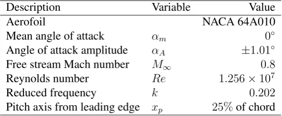
of the widely used cases to validate transonic CFD codes. The experimental work was carried out by Davis [25], Alonso et al. [18] as well as by Chen et al. [26] in order to validate their CFD codes. Table 1 gives the operating conditions for this case.

Description Variable Value

Aerofoil NACA 64A010

Mean angle of attack αm 0◦

Angle of attack amplitude αA ±1.01◦

Free stream Mach number M∞ 0.8

Reynolds number Re 1.256×107

Reduced frequency k 0.202

[image:10.595.154.442.160.278.2]

Pitch axis from leading edge xp 25%of chord

Table 1: Characteristics of test case A.

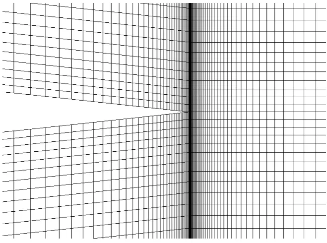
In this case GMSH has been used [27] instead of using one of OpenFOAM meshing utilities. GMSH has a graphical user interface which gives more control, and thus accelerates the mesh generation process. Figures 1 and 2 show the complete mesh and the mesh around the sharp trailing edge respectively. The computational domain is

15c×10cwith39,006grid cells.

[image:11.595.138.458.107.328.2]

Figure 1: C-mesh type around NACA 64A010

[image:11.595.132.462.385.630.2]

-0.1 -0.05 0 0.05 0.1

-1.5 -1 -0.5 0 0.5 1 1.5

Cl

Angle of Attackα

[image:12.595.118.469.109.317.2]

Experimental [25] OpenFOAM

Figure 3: Instantaneous lift Coefficient

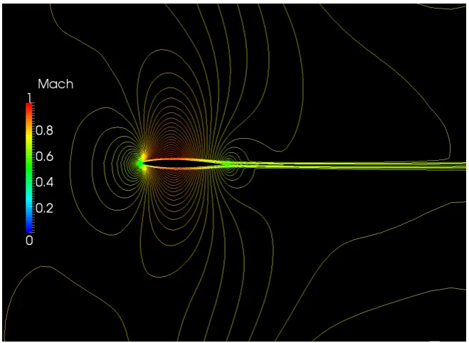
Figure 4: Mach Contours atα= 1.01◦

4.2

Case B: Self-Sustained NACA 64A010

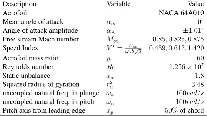
[image:12.595.133.463.369.610.2]

fol-lows the one which was introduced by Isogai [5, 6]. The modelling for each condition was done using three stages, namely, fixed aerofoil, pitching aerofoil around the elas-tic axis and finally self-sustained aerofoil. The same mesh from case A was used to save computational time. A fifth-order Runge-Kutta with adaptive time step devel-oped by Cash and Karp [29] was selected. It is one of the OpenFOAM ODE solvers for non-stiff systems.

Description Variable Value

Aerofoil NACA 64A010

Mean angle of attack αm 0◦

Angle of attack amplitude αA ±1.01◦

Free stream Mach number M∞ 0.85,0.825,0.875

Speed Index V∗ = U∞ ωαb

√

µ 0.439,0.612,1.420

Aerofoil mass ratio µ 60

Reynolds number Re 1.256×107

Static unbalance xα 1.8

Squared radius of gyration r2

α 3.48

uncoupled natural freq. in plunge ωh 100rad/s

uncoupled natural freq. in pitch ωα 100rad/s

[image:13.595.127.469.204.396.2]

Pitch axis from leading edge xp −50%of chord

Table 2: Characteristics of test case B.

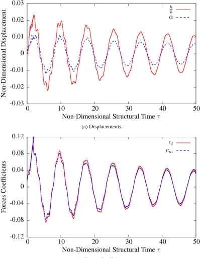
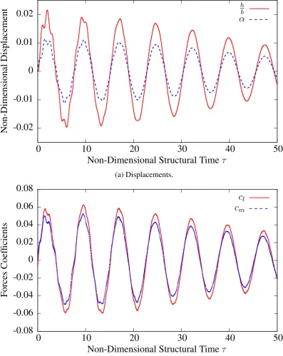
Figures 5, 6 and 7 show the responses and the forces for the three operating condi-tions. It is clear that Figure 5 represents a damped response, whereas Figure 7 shows a divergent response. Both are in very good agreement with [18, 26]. It was expected that Figure 6 would predict the flutter point as reported by Alonso et al. [18], but as it turned out the flutter point was missed only by a small margin. Nevertheless, the trend to predict the flutter speed is sufficiently clear.

5

Conclusions

-0.03

-0.02

-0.01

0

0.01

0.02

0.03

0

10

20

30

40

50

Non-Dimensional

Displacement

Non-Dimensional Structural Time

τ

h b

α

(a) Displacements.

-0.12

-0.08

-0.04

0

0.04

0.08

0.12

0

10

20

30

40

50

F

orces

Coef

ficients

Non-Dimensional Structural Time

τ

c

l

c

m

[image:14.595.94.493.150.664.2]

(b) Forces Coefficients.

-0.02

-0.01

0

0.01

0.02

0

10

20

30

40

50

Non-Dimensional

Displacement

Non-Dimensional Structural Time

τ

h b

α

(a) Displacements.

-0.08

-0.06

-0.04

-0.02

0

0.02

0.04

0.06

0.08

0

10

20

30

40

50

F

orces

Coef

ficients

Non-Dimensional Structural Time

τ

c

l

c

m

[image:15.595.95.493.157.657.2]

(b) Forces Coefficients.

-0.4

-0.2

0

0.2

0.4

0

10

20

30

40

Non-Dimensional

Displacement

Non-Dimensional Structural Time

τ

h b

α

(a) Displacements.

-1

-0.5

0

0.5

1

0

10

20

30

40

F

orces

Coef

ficients

Non-Dimensional Structural Time

τ

c

l

c

m

[image:16.595.93.488.149.668.2]

(b) Forces Coefficients.

References

[1] R. Bisplinghoff, H. Ashley, R. Halfman, Aeroelasticity, Dover Books on Aero-nautical Engineering Series. Dover Publications, 1996.

[2] Y.C. Fung, An Introduction to the Theory of Aeroelasticity, Dover Phoenix Edition: Engineering. Dover Publications, Incorporated, 2002.

[3] R. Clark, D. Cox, H. Curtiss, E. Dowell, J. Edwards, K. Hall, D. Peters, R. Scan-lan, E. Simiu, F. Sisto, A Modern Course in Aeroelasticity, Solid Mechanics and Its Applications. Kluwer Academic Publishers, 2006.

[4] W. Rodden, Theoretical and Computational Aeroelasticity, Crest Publishing, 2011.

[5] K. Isogai, “On the Transonic-Dip Mechanism of Flutter of a Sweptback Wing”,

AIAA Journal, 17(7): 793–795, July 1979.

[6] K. Isogai, “Transonic dip mechanism of flutter of a sweptback wing. II”, AIAA Journal, 19(9): 1240–1242, Sept. 1981.

[7] O.O. Bendiksen, “Review of unsteady transonic aerodynamics: Theory and ap-plications”, Progress in Aerospace Sciences, 47(2): 135–167, Feb. 2011.

[8] O.O. Bendiksen, G. Seber, “Fluidstructure interactions with both structural and fluid nonlinearities”, Journal of Sound and Vibration, 315(3): 664–684, Aug. 2008.

[9] R.M. Bennett, J.W. Edwards, “An overview of recent developments in computa-tional aeroelasticity”, AIAA paper, (98-2421), 1998.

[10] G.P. Guruswamy, “A review of numerical fluids/structures interface methods for computations using high-fidelity equations”, Computers & structures, 80(1): 31–41, 2002.

[11] D.M. Schuster, D.D. Liu, L.J. Huttsell, “Computational aeroelasticity: success, progress, challenge”, Journal of Aircraft, 40(5): 843–856, 2003.

[12] H.I. Kassem, X. Liu, J.R. Banerjee, “Flutter Analysis using a Fully Coupled Density Based Solver for Inviscid Flow”, in B.H.V. Topping, P. Ivnyi, (Edi-tors), ”Proceedings of the Twelfth International Conference on Computational Structures Technology”. Civil-Comp Press, Stirlingshire, UK, Paper 146, 2014. doi:10.4203/ccp.106.146

[13] “OpenFOAM-2.3.0 user guide”, February 2014.

[14] “OpenFOAM-2.3.0 release notes”, February 2014. http://www. openfoam.org/version2.3.0/index.php

[15] J.H. Ferziger, M. Peri´c, Computational methods for fluid dynamics, Volume 3, Springer Berlin, 1996.

[16] H.K. Versteeg, W. Malalasekera, An Introduction to Computational Fluid Dy-namics: The Finite Volume Method, Pearson Education Limited, 2007.

[17] C.J. Greenshields, H.G. Weller, L. Gasparini, J.M. Reese, “Implementation of semi-discrete, non-staggered central schemes in a colocated, polyhedral, finite volume framework, for high-speed viscous flows”, International journal for numerical methods in fluids, 63(1): 1–21, 2010.

AIAA paper, (94-0056), 1994.

[19] F. Liu, J. Cai, Y. Zhu, H.M. Tsai, A.S. F. Wong, “Calculation of Wing Flutter by a Coupled Fluid-Structure Method”, Journal of Aircraft, 38(2): 334–342, Mar. 2001.

[20] L.F.G. Marcantoni, J.P. Tamagno, S.A. Elaskar, “HIGH SPEED FLOW SIMU-LATION USING OPENFOAM”, inMec´anica Computacional Vol XXXI, pages 2936–2959. Asociaci´on Argentina de Mec´anica Computacional, 2012.

[21] A. Kurganov, E. Tadmor, “New High-Resolution Central Schemes for Nonlinear Conservation Laws and ConvectionDiffusion Equations”, Journal of Computa-tional Physics, 160(1): 241–282, 2000.

[22] H. Jasak, Z. Tukovic, “Automatic mesh motion for the unstructured finite volume method”, Transactions of FAMENA, 30(2): 1–20, 2006.

[23] H. Jasak, “Dynamic Mesh Handling in OpenFOAM”, 43rd AIAA Aerospace Sciences Meeting and Exhibit, pages 1–10, 2008.

[24] H. Jasak, A. Jemcov, Z. Tukovic, “OpenFOAM: A C++ library for complex physics simulations”, in International Workshop on Coupled Methods in Nu-merical Dynamics, IUC, Dubrovnik, Croatia, pages 1–20, 2007.

[25] S.S. Davis, “NACA 64A010 (NASA Ames Model) oscillatory pitching”,

AGARD Report, 702, 1982.

[26] X. Chen, G. Zha, Z. Hu, M.T. Yang, “Flutter Prediction Based on Fully Cou-pled Fluid-Structural Interactions”, in9th National Turbine Engine High Cycle Fatigue Conference, 2004.

[27] C. Geuzaine, J.F. Remacle, “Gmsh: A 3-D finite element mesh generator with built-in pre-and post-processing facilities”, International Journal for Numerical Methods in Engineering, 79(11): 1309–1331, 2009.

[28] M. McMullen, A. Jameson, J. Alonso, “Application of a non-linear frequency domain solver to the Euler and Navier-Stokes equations”, AIAA paper, 120, 2002.