Estimation of Vector Fields in Unconstrained and Inequality Constrained Variational Problems for Segmentation and Registration

City, University of London Institutional Repository

Citation

:

This is the accepted version of the paper.

This version of the publication may differ from the final published

version.

Permanent repository link:

Link to published version

:

Copyright and reuse:

City Research Online aims to make research

outputs of City, University of London available to a wider audience.

Copyright and Moral Rights remain with the author(s) and/or copyright

holders. URLs from City Research Online may be freely distributed and

linked to.

Estimation of Vector Fields in Unconstrained and

Inequality Constrained Variational Problems for

Segmentation and Registration

Gozde Unal*,

Greg Slabaugh

Intelligent Vision and Reasoning

Siemens Corporate Research

Princeton, NJ 08540

*Corresponding author: [email protected]

Abstract

Vector fields arise in many problems of computer vision, particularly in non-rigid registration. In this paper, we

develop coupled partial differential equations (PDEs) to estimate vector fields that define the deformation between

objects, and the contour or surface that defines the segmentation of the objects as well. We also explore the utility of

inequality constraints applied to variational problems in vision such as estimation of deformation fields in non-rigid

registration and tracking. To solve inequality constrained vector field estimation problems, we apply tools from

the Kuhn-Tucker theorem in optimization theory. Our technique differs from recently popular joint segmentation

and registration algorithms, particularly in its coupled set of PDEs derived from the same set of energy terms for

registration and segmentation. We present both the theory and results that demonstrate our approach.

Index Terms

variational problems, equality constraints, inequality constraints, vector fields, nonrigid registration, joint

I. INTRODUCTION

Many problems in computer vision and image processing can be posed as variational problems. Exam-ples are image filtering, segmentation, registration, and tracking, which have been extensively solved with variational methods and nonlinear partial differential equations (PDEs). The solutions of such problems generally take the form of images, curves, surfaces, and vector fields, and are sought through an evolution equation defined by a PDE. Usually, an initial estimate of the solution is deformed through a given PDE, which in most cases is derived from optimization (typically minimization) of an energy functional, and occasionally from local heuristics.

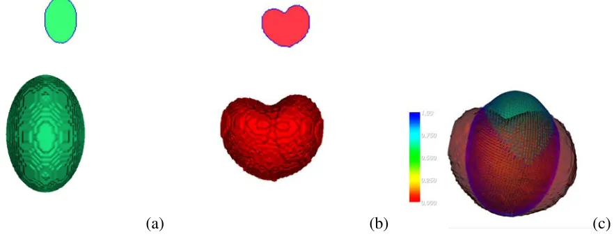
Deformation or displacement fields arise in registration, segmentation, and tracking problems, partic-ularly in the case of multiple image data when a general coordinate transformation is defined between the two image domains. This mapping is usually described through a vector field that transforms one of the image domains to another one. A particular application occurs when a target structure deforms differently in various image volumes, and a joint registration and segmentation approach would be useful if we would like to utilize all the information coming from the multiple images that may be available. In this case, the segmentation and registration processes operate in a coupled way to help each other for an accurate content extraction goal. For instance, in the simplest case, two image volumes consisting of binary regions are shown in Figure 1 and the goal is to segment the 3D shape from the given multiple image volumes and simultaneously capture the deformation among these volumes as shown in (c).

(a) (b) (c)

Fig. 1. (a)-(b) Two binary image volumes which have a non-rigid correspondence (visualized by their zero level sets in 3D and a 2D

cross-section shown at the top). (c) The estimated surfaces with the vector field on the green surface correctly pointing toward the red surface.

that are computed from a sequence of images using temporal and spatial object brightness constraints such as the optical flow equation [17].

As a variational framework is utilized to find solutions to such problems, in some cases, the subset of solutions may be defined by a set of implicit constraints, for example by nonlinear equality or inequality relations. This brings up the question as how to solve variational problems that have constraints. In the case of differential equation constraints, for instance, the solution space has to be confined locally over the domain of the problem, and this turns out to be a non-trivial task.

The popularity and usefulness of variational methods support the efforts for bringing new mathematical tools to the attention of the computer vision community. A general tool that we believe will be useful in variational problems in computer vision and related fields is constrained variational calculus tools for problems such as estimation of a deformation or displacement vector field with inequality constraints.

single contour and its deformation field with certain inequality constraints.

For solving variational problems that have constraints, the method of direct substitution is the most straightforward procedure, where the constraint equation, if possible, is substituted into the integrand; then the problem is converted into an unconstrained problem. However, this is not possible for the majority of the constrained problems.

Generally, a popular tool that arises is Lagrange multipliers, which always simplify a difficult constrained problem. It should be noted that in a more sophisticated approach, Lagrange multipliers take the form of functions, not the form of constant numbers [19]. When the Lagrange multiplier is a function of the independent variables, this brings an added complication that was not encountered in the types of constraints previously used in the computer vision community.

Constrained problems that are well studied in history of mathematics are: geometrically constrained problems such as the isoperimetric problem, geodesic problems, like the brachistochrone problem, and control theory [10]. Differential forms arise in many constraints, such as the divergence constraint for incompressibility of fluids, or divergence and curl operators in electromagnetism.

A. Related Work

the prior shape. The segmentation energy is separately involved as a boundary and region based energy model. In [33], similarly, a boundary based energy or a Mumford-Shah energy is utilized in conjunction with a distance to a shape prior to which the evolving contour is transformed by a rigid motion. In the same work, the authors also presented an intensity-based PDE which evolves a source image towards a target image, and a coupling PDE to solve for the coordinate transformation from source to the target. This approach however involves a pre-segmentation step, hence is not a joint segmentation and registration approach. Using different criteria for segmentation and rigid registration, an iterative/sequential manner has been carried out in a Bayesian framework in [36]. The same idea of simultaneous segmentation and rigid registration with a prior shape model has been applied to time-varying data for motion estimation and segmentation of moving structures, particularly in cardiac imaging [14]. An active region model based on classical snake nodal constraints with a displacement field defined over the nodes is utilized for again a combined segmentation and motion tracking goal in heart imaging. Almost all of the methods listed above involve only rigid registration as the transformation between two shapes or images.

Wang and Vemuri in [34], also proposed a joint non-rigid registration and segmentation, however, this technique is different from ours in that the registration and segmentation terms in the energy are separate but the coupling between these two operations is only introduced by a third term that checks the distance between the evolved curve and the curve transformed with the deformation field.

however the field is only over the surface. In addition, we also solve for the segmentation in multiple images jointly with the registration.

Analysis and decomposition of vector fields, which are useful functions in many applications, have been studied extensively. For smooth vector fields, Helmholtz-Hodge decomposition [1] provides an intuitive decomposition of a vector field into its components: a rotation-free component, a divergence-free component, and the residuals that are sometimes called the harmonic component. Projection operators were introduced to restore vector field properties such as divergence, curl, and hyperbolic components in [30]. A variational approach was taken in [27] where vector fields on triangulated surfaces were decomposed into a rotation-free, divergence-free and a harmonic component. A multi-scale extension for discrete vector fields was done in [31]. A discrete exterior calculus theory specifically to work with discrete vector fields and operations such as a discrete Hodge decomposition was developed in [13].

Related recent work on constrained variational problems include widely used constraints on vector fields that are referred to as smoothness constraints [2], [7], which only serve the purpose of regularization of the flow. Chefd’hotel et al. utilized matrix constraints such as unit-normness, orthogonality and positive-definiteness in their work that extends and generalizes the variational framework in computer vision from scalar-valued functions to matrix-valued functions [8]. A global constraint on the magnitude of the vector field is utilized in [26] to prevent the vector field from having unnecessarily large amplitudes. In [18], optical flow fields were estimated with a penalty of departure from rigidity, however, without any local inequality constraints like we present here. For myocardium segmentation, image edge and velocity measurements from MR intensity and MR phase contrast images are used to constrain the curve propagation in [35], however this method does not involve a variational constraint approach. An excellent text on image registration, regularization and its numerical solutions can be found in [21].

B. Our Contributions

paper is that we utilize the Kuhn-Tucker theorem to solve for inequality constrained problems in computer vision. Specifically, the solutions to these problems involve locally constrained minimizations with a Lagrange multiplier function that varies with respect to the independent variables. We investigate new avenues with inequality constrained problems that may lead to improved solutions for the estimation of vector fields in problems such as segmentation, registration, and tracking.

A second contribution is the generalization of the joint segmentation and registration work of Yezzi et al. [38], which involved only finite dimensional registrations, but had not foreseen an extension to infinite dimensions. However, a best rigid fit among image volumes will not result in a correct registration in various imaging applications. Therefore, we start with the same joint segmentation and registration idea however improve it to account for more general problems of registration among anatomical structures defined by a deformation field between target regions. The applications are vast such as structures in different MR image sequences (for instance T1 and T2 weighted) or pre and post contrast agent MR images or images of a patient at different time points or images of different patients as well as images of different modalities.

The organization of the paper is as follows. In Section II, we give the fundamentals of the constrained problems in optimization. Section III presents the application of constrained calculus of variations problems in computer vision and derives the specific PDEs in Section IV. Section V presents the experimental results and conclusions.

II. CONSTRAINEDPROBLEMS IN THECALCULUS OFVARIATIONS

A. Fundamentals

The vector field u ∈ Y = C2(Ω,Rn) is searched in a set U of admissible functions such that it minimizes an energy functional I:U −→R of the form:

F(u) =

Ω

f(x,u, Du)dx (1) subject to the functional constraints Ψ(x,u, Du) = 0, (2)

Φ(_x,u, Du)≤0. (3)

where D denotes the Jacobian of u.

Definition A function u that satisfies all the functional constraints is said to be feasible.

Definition A point at which the Gateaux differential of a functional F vanishes, i.e., δF(u∗;h) = 0 for all the admissible variations h, is called a stationary point 1_.

From the above definition, it is clear that the extrema of a functional F occur at stationary points. When the vector space X is normed, a more satisfactory definition of a differential is given by the

Fr´echet differential.

Definition If for each variation h ∈ X there exists F(h) such that lim_||h||→0||F(u +h)−F(u)− F(h)h||/||h|| = 0, then F is said to be Fr´echet differentiable and F is said to be the Fr´echet differential of F (see [19] for more details). In the special case, which corresponds to our case, where the transformation F is simply a functional on the space X, F is called the gradient of F, also denoted by ∇F.

B. Equality Constrained Problems

Theorem 1: (Lagrange Multiplier) If the continuously Fr´echet differentiable functional F in Eq. (1) has a local extremum under the equality constraint (2), Ψ(x,u, Du) = 0, at the regular point u∗, then

1

If F is a functional on a vector spaceX, the Gateaux differential ofF, if it exists, isδF(x;h) = _dtdF(x +th)|t=0, and for each

fixedx ∈X,δF(x;h)is a functional with respect to the variableh ∈X. The Gateaux differential generalizes the concept of directional

there exists a function μ∈C2(Ω,Rn) such that the Lagrangian functional

F(x,u, Du) +μ(x)Ψ(x,u, Du) (4)

is stationary at u∗, i.e., F(u∗) +μΨ(u∗) =0.

The intuition with this result is that F(u∗), the gradient of F, must be orthogonal to the null space of

Ψ_(u∗_{), that is orthogonal to the tangent space.}

C. Inequality Constrained Problem

A fundamental concept that provides much insight and simplifies the required theoretical development for inequality constrained problems is that of anactive constraint. An inequality constraint Φ(x,u, Du)

is said to be active at a feasible solution u if Φ(u) = 0 and inactive at u if Φ(u)<0. By convention, any equality constraint Ψ(u) = 0 is active at any feasible point. The constraints active at a feasible point u in the set of admissible functions restrict the domain of feasibility in neighborhoods of u. On the other hand, inactive constraints, have no influence in neighborhoods ofu. Inequalities are treated by determining which of them are active at a solution. An active inequality then acts just like an equality except that its associated Lagrange multiplier can never be negative.

Definition A pointu∗ is aregular pointif the gradients of the active constraints are linearly independent.

Theorem 2: (Kuhn-Tucker) Let u∗ be a relative minimum point for the problem of minimizing Eq. (1) subject to the constraint (3), and suppose u∗ is a regular point for the constraints. Then, there is a function λ∈C2(Ω,Rn) with λ(x)≥0 such that the Lagrangian

F(x,u, Du) +λ(x),Φ(x,u, Du) (5)

is stationary at u∗. Furthermore,

Note that now there are two unknown functions to be estimated: the function u(x) and the Lagrange multiplierλ(x)that both vary over the domainΩ. The second necessary condition (6) in the Kuhn-Tucker theorem in addition to the first necessary condition (5) are enough to solve for the two unknowns.

Kuhn-Tucker reformulations for converting the constrained problems into unconstrained problems are presented in [5], [15]. In addition, an interesting approach is presented in [16] with new numerical solutions to the integral forms of the Euler-Lagrange equations for constrained problems.

Types of Constraints: There are multitude of different constraint functions that can be used in constraining a cost functional. There is no clear classification, but the ones we came across are as follows. Local constraints are also called as “algebraic constraints”, i.e.G(x) = 0(in mechanics called “holonomic constraints”). There are “differential equation constraints”, which we are interested in,G(x, u, u) = 0are local constraints (in mechanics called “non-holonomic constraints”), and result in a Lagrange multiplier, which is a function of the independent variable, like λ(x). On the other hand, the “integral constraints” are global constraints, and result in a single constant Lagrange multiplier number λ.

III. APPLICATIONS

For specific applications of the above theorems, we will show in the framework of the calculus of variations, specific examples that will be useful in various computer vision scenarios. Because the case of equality constraints is a special case for the inequality constraints, we opted to study inequality constrained problems as applied to problems in segmentation, registration, and tracking.

In the framework of calculus of variations with inequality constraints, our problem is to minimize

F(u) =

Ω

f(x,u, Du)dx (7)

subject to Φ(x,u, Du)≤0 (8)

The first necessary condition is obtained as follows:

∂

∂t{F(x,u +th, D(u +th)) + λ(x),Φ(x,u +th, D(u +th)) } |t=0 =0. (9)

Hence, we look for the differential of the new Lagrangian J =F+< λ,Φ>:

δJ(u;h) = ∂ ∂t

Ω

f(x,u +th, D(u +th))dx

+ ∂

∂t

Ω

Φ(_x,u +th, D(u +th))λ(x)dx. (10)

By the chain rule, the differentialδJ(u;h)can be obtained as the first necessary condition when equated to zero:

δJ(u;h) =

Ω

f_u(x,u, Du)hdx +

Ω

f_Du(x,u, Du)Dhdx

+

Ω

Φ_u(_x,u, Du)hλ(x)dx +

Ω

Φ_Du(_x,u, Du)Dhλ(x)dx. (11)

In this equation, _u and _Du in the subscripts denote the variation of a functional, e.g. of f and Φ with respect to the functions u and Du. Integrating (11) by parts,

Ω

Ω

f_udx −f_Du +

Ω

Φ_udλ(x)−Φ_Dudλ

Dhdx =0 (12)

for all variations h vanishing at the boundary of the bounded domain Ω. The resulting Euler-Lagrange equation in its integral form is thus

Ω

f_udx−f_Du+

Ω

Φ_udλ(x)−Φ_Dudλ=0. (13)

In its more familiar differential form, the Euler-Lagrange equations reduce to:

f_u−∇f_Du+Φ_uλ(x)−Φ_Du∇λ(x)=0. (14)

The second necessary condition from the Kuhn-Tucker theorem (6) is given by the equation:

Ω

Φ(_x,u, Du)λ(x)dx =0, (15)

active over the domain Ω only when the equality is satisfied, and vanishes when the strict inequality is satisfied, that is:

Φ(_x,u, Du) < 0(inactive constraint)→λ(x) = 0 (16)

Φ(_x,u, Du) = 0(active constraint)→λ(x)>0. (17)

A. Algorithm

We summarize the proposed algorithm for clarity. The coupled equations consisting of (14) with the auxiliary equation (15) forms a complete set of equations to solve for the unknowns u(x) and λ(x)

over the domain Ω. The specifics of the cost functionalf will be given in the next subsections. To set up the iterations for the PDEs, an artificial time variable t is introduced, and the PDE from Eq. (14) to be solved is:

∂u(x, t)

∂t =−fu+∇fDu−Φuλ(x, t)+ΦDu∇λ(x, t). (18)

Using the time as a new variable, the auxiliary equation in (15) becomes

Ω

Φ(_x,u(x, t), Du(x, t))λ(x, t)dx =0 . (19)

Without the specifics of the functionals f and Φ, the general algorithm proceeds as follows: 1) At time t₀ = 0, start with a fixed initial value u0 =u(t₀) that satisfies

Φ(_x,u(x, t₀), Du(x, t₀))<0. Then initial value ofλ(x, t)is automatically fixedλ0 =λ(x, t₀) = 0.

2) At time step, t_k=kΔt, solve for uk=u(x, t_k) from Eq. (18) using uk−1 and λk−1. 3) Solve for λk from Eq. (19) usinguk.

4) Repeat the steps 2-3 until convergence.

B. Solving Equation (19)

Φ(_x) is non-zero. Of course, we require the gradient of λ over the space in our PDE (18), and the delta function is differentiable only when it is viewed as a generalized function. For simplifying the problem, we replace the delta function by a regularized delta function

λ(x) =Kδ(Φ(x)≥0(x))≈Kξ(r), (20)

where K is a strength factor, and the above yields a well-defined and differentiable Lagrange multiplier function λ(x) as we require. The ξ(·) is a regularized distribution that is supported by a finite cross-sectional area in Rn. It can also be thought as n −dim blobs around each point x in space, where

r =|x −x₀|, is the distance from the center of the blob x₀. The distribution function ξ(x) = _σπ₂g(_σr)

is a regularization of the delta function, normalized so that its integral over the space is equal to unity. Here, σ is the radius of the blob, which is a measure of the extent of the spread of the blob, and g is a dimensionless distribution that vanishes at ∞. Note that in the limit as σ →0, ξ reduces to the delta function.

A choice for theg function is given by g(w) = _π1₂e−w2. For n = 2, for instance, the 2D delta function is separable, and will be computed from δ(x, y) = δ(x)δ(y). In addition, we smooth the final λ(x)

function by a Gaussian filter to ensure that its gradient is regular.

IV. SPECIFICS OF THE CONSTRAINEDPDE (18)

Generally speaking, the functional f in (18) consists of two types of terms:

f =fi+fr (21)

wherefi is an image- and data-driven term, andfr is a regularizing term on the unknown function, here

u.

A. Regularizer

The simplest choice of a regularizer functional fr is the Dirichlet integral:

fr=

Ω||

Trace(DuDuT)||dx (22)

that yields a pure diffusion operator in the PDE, i.e., div (Du), and hence assumes a smoothly varying vector field over the whole Ω domain. More sophisticated regularizing integrals that respect the discon-tinuity over the high image gradients are proposed such as the anisotropic diffusion term in [2]. Other forms of regularizers and more general matrix-valued functions can be found in [7], [11]. We will utilize the regularization operator:

div (Du) (23)

in our specific PDEs.

B. Image-Dependent Functionals

The data-driven term of the cost functional is chosen depending on the vision application.

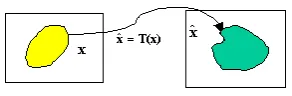
1) A joint non-rigid registration and segmentation approach: For segmentation of a structure appearing in multiple domains, Unal et al. [32] presented a joint non-rigid registration and segmentation technique that utilized an infinite-dimensional transform xˆ =T(x) where each point in domain Ωcan move freely to a point in domain Ωˆ as depicted in Figure 2.

Fig. 2. Non-rigid mapping between two images defined through the coordinate transformation:T(x) =x+u.

We briefly summarize this technique as follows. Given two image volumes, I : Ω ∈ Rn −→ R and

ˆ

I : ˆΩ ∈ Rn −→ R, we denote the transformation that deforms one of the images to the other one by:

ˆ

or 3). The goal is to find a surface S ∈Ω that deforms on the first image I whereas a surface Sˆ ∈ Ωˆ corresponding to the mappingSˆ =T(S)deforms on the second image Iˆ. Both surfaces move according to a generic image region-based energy functional defined over both image domains depending on region descriptors for the unknown foreground region, fi,f, and the background region, fi,b:

E(u,S)=

Ω

fi,f(x)χf(x)dx +

Ω

fi,b(x)(1−χf(x))dx

+

ˆΩ

ˆ

fi,f( ˆx)χf( ˆx)dxˆ +

ˆ Ω

ˆ

fi,b( ˆx)(1−χf( ˆx))dxˆ (24)

where χf denotes an indicator function for the foreground region over an image domain, fˆi,f and fˆi,b

are the region descriptors for the foreground and the background in the transformed domain Ωˆ. Note that in this case there is an additional unknown, the boundaries between the foreground and the background regions, i.e. the surfaceS for segmentation, and a proper regularizer onS is also introduced through the surface area integral _S dA that induces a curvature term in the resulting segmentation PDE.

The solutions to the minimization problems are given by:

˜

S = arg min

S E(S,u), and u˜ = arg minu E(S,u) (25)

The surface evolution is given by:

∂S ∂t =f

i_{(x)N + ˆf}i_{(x +u(x))N}ˆ _{+κN. (26)}

Note that fi =fi,f −fi,b, and fˆi = ˆfi,f −fˆi,b, N is the normal vector to the surface S, and Nˆ is the normal vector to the transformed surface Sˆ, and κ is the curvature function for the surface S.

For registration evolution, the only part of the energy functional in Eq. (24) that is taken into account is:

E(u)=

Ω

ˆ

fi,f(x +u(x))χf(x +u(x))

Ff₍x₊u₍x₎₎

dx+

Ω

ˆ

fi,b(x +u(x))(1−χf(x +u(x)))

Fb₍x₊u₍x₎₎

dx (27)

displacement field u which varies over space. The contributing term to our constrained PDE (18) from the image functional is then:

∂u(x, t)

∂t = ∇u

ˆ

fi,f(x +u(x))χf(x +u(x))+∇_ufˆi,b(x +u(x))(1−χf(x +u(x)))

+ ˆfi(x +u(x))∇_u(χf(x +u(x))) (28)

u(_x,0) = u_o(x).

For the third term above, the derivative of the indicator functionχ with respect to u is intuitively a delta function over the boundaries between the foreground and the background region, and is defined in the sense of distributions. In practice regularized versions of a heaviside function H and a delta function δ

are used, particularly within a level set implementationφ : Ω−→R which represents S as its zero level set [6]:

∂u(x, t)

∂t = ∇u

ˆ

fi,f(x +u(x))H( ˆφ(x +u(x)))+∇_ufˆi,b(x +u(x))(1−H ( ˆφ(x +u(x))))

+ ˆfi(x +u(x)) δ ( ˆφ(x +u(x)))∇φˆ(x +u(x)) (29)

u(_x,0) =u_o(x).

A special case for the image dependent functional fi can be chosen as a simplified Mumford-Shah model [22], that is the piecewise constant model by Chan-Vese [6] that approximates the target regions in a given image I by the mean statistics. For instance, for a foreground region with a statistic m_f, and a background region with a statistic m_b, the specific form of fi becomes

fi(x,u) =(I(x +u)−m_f)2χf(x) +(I(x +u)−m_b)2(1−χf)(x).

With the piecewise (p-w) constant model for the target regions that are to be segmented and registered in images I and Iˆ, the region-based term in the energy, and the gradient terms are given by:

ˆ

f= ˆfi,f −fˆi,b= 2( ˆm_f −mˆ_b)(mˆf + ˆmb

2 −Iˆ(x+u(x))),

∇ufˆi,f = 2( ˆI(x +u(x))−mˆ_f)∇Iˆ(x +u(x))

where mˆ_f and mˆ_b are the mean of the image intensities inside and outside the surface mapped onto the second image volume domain respectively. These expressions can be inserted into (28) to obtain the PDE, which flows in the gradient descent direction, for evolution of non-rigid registration field for the p-w constant region model:

∂u(x, t)

∂t = −( ˆmf −mˆb)[

( ˆm_f + ˆm_b)

2 −Iˆ(x +u(x))] δ( ˆφ(x +u(x)))∇φˆ(x +u(x))

−( ˆI(x +u(x))−mˆ_f)∇Iˆ(x +u(x)) H ( ˆφ(x+u(x)))

−( ˆI(x +u(x))−mˆ_b)∇Iˆ(x +u(x))(1−H ( ˆφ(x +u(x)))) (30)

u(_x,0) =u_o(x) =0,

where a zero vector field initialization is adequate in solving the PDE without any prior knowledge of the true vector field u.

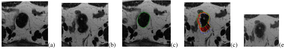
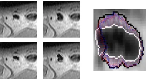
In Figure 3, two different slices of an MR image sequence depict a dark structure in the middle, and which is jointly registered and segmented by the PDEs (30), (26), and (23). The result of deforming the second image region of interest (that is around and inside the contour) with the estimated vector field towards the first image particularly shows the success of the estimation.

(a) (b) (c) (c) (e)

Fig. 3. A 2D MR image pair at different slice levels (a,b). The structure’s deformation is recovered by the Eqns. (30),(26)) depicted with

the vector field whose direction goes from red to blue(c,d), i.e., green contour to yellow contour. The second image is deformed by the

estimated vector field (e).

surface from the outside by the given threshold. For this purpose we use the following speed function:

ˆ

f = ( ˆm_f −mˆ_b)(T −Iˆ(x +u(x))) (31) where the mˆf+ ˆmb

2 quantity in “Chan-Vese” flow is replaced by an arbitrary threshold T. For this speed

function we use the image terms on right hand side of the following PDE for updating the vector field:

∂u(x, t)

∂t = −( ˆmf−mˆb)(T−Iˆ(x+u(x))) δ( ˆφ(x+u(x)))∇φˆ(x +u(x))

u(x,0) = uo(x) =0, (32)

applied to the boundary term only.

For a tracking application, the image-based functional term can also be chosen as an image matching penalty (I(x)−Iˆ(x +u(x)))2dx, as in the popular optical flow equation. Then the image matching term becomes:

∂u(x, t)

∂t =−(I(x)−

ˆ

I(x +u(x))) ∇( ˆI(x +u(x))). (33)

One can note that although the flows are presented for between two image domains, this idea can be extended to multiple coordinate spaces to non-rigidly register a single common contour with multiple target objects.

C. Divergence Inequality Constraints

A natural constraint on the displacement vector field u is a constraint on the its divergence divu. The divergence of a 2-dimensional vector field u = (ux, uy) is defined as the trace of its Jacobian matrix

Du =

⎡ ⎢ ⎢ ⎣ ∂ux ∂x ∂u x ∂y ∂uy ∂x ∂u y ∂y ⎤ ⎥ ⎥

⎦. (34)

Let us suppose we want to constrain the divergence of a vector field by a constant, say c, then the constraint function becomes

where c is a constant scalar function. To obtain the constrained PDE in this specific case, we write the differentials of Φ to find

Φ_Du = ∂

∂Du(Trace(Du)−c) =Id (36)

whereIddenotes the identity matrix. Therefore, for the goal of constraining divergence of the vector field from below, say by a given constant c₁, and from above, say by a given constant c₂ in a given variational vision problem, we set up two constraint functions:

Φ1_{(x, Du) = c}

1−div u(x)≤0 (37)

Φ2_{(x, Du) = div u(x)−c}

2 ≤0. (38)

Then we define two Lagrange multiplier functions, λ1(x) and λ2(x), which contribute to the specific form of our constrained PDE (18) as the operators

Φ1

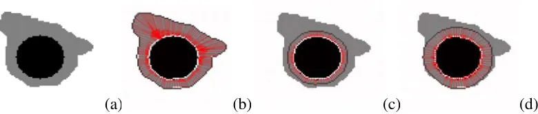
Du∇λ1(x) + Φ2Du∇λ2(x) = −∇λ1(x) +∇λ2(x). (39) Figure 4 depicts an application of the divergence constraints (37-38) on a vector field estimation. Here, as compared to joint registration and segmentation application, the idea is to use one contour and a vector field on the same image I. The vector field that defines the mapping between the inner boundary around the black circular region and the outer boundary can be easily estimated using the PDE terms in Eq. (30) and regularizer term in (23). The resulting segmentation (contour) and the vector field are shown in (b). To demonstrate the effect of the inequality constraints on the divergence of the vector field, we apply the constraints c₁ ≤divu ≤ c₂, with c₁ = 0.1 and c₂ = 0.3. The initialized vector field that satisfies the constraint divu =c₁ is shown in (c). Figure 4-(d) shows the result of the evolution of the PDE (39) with the auxiliary equation (19) to solve for the Lagrange multiplier functions λ1 and λ2.

(a) (b) (c) (d)

Fig. 4. The divergence inequality constraint on the vector field that maps the inner boundary towards the outer boundary demonstrated on

the image in (a) (negative of the vector field is depicted). (b) Evolution without any constraint. (c) Initialized vector field with a divergence

inequality constraint. (d) Resulting vector field with divergence constrained evolution.

D. Curl Inequality Constraints

A complementary idea to the divergence constraint is the usage of a curl constraint on a vector field. In fluid dynamics, curl of a vector field is defined as the vorticity. The intuition then in a tracking application is to put vorticity constraints on the vector field.

The curl constraint function can be written as

Φ(x,u, Du) = Trace J (Du)−v ≤0 (40)

where J denotes a 90 degree rotation on the Jacobian matrix, and v denotes a given vorticity of the vector field. Taking derivative of Φ w.r.t. u in this case yields:

Φ_Du = ∂

∂Du(Trace J (Du)−v) =J . (41)

Similar to the divergence constraints in the previous section, vorticity of a vector field can be limited from both below and above with two values of vorticity v₁ and v₂

Φ1_{(x, Du) = v}

1−curl u(x)≤0 (42)

Φ2_{(x, Du) = curl u(x)−v}

2 ≤0. (43)

Then we define two Lagrange multiplier functions,λ1(x)andλ2(x), which contribute to our constrained PDE (18) in the specific form of the operators

Φ1

Figure 5 shows two synthetically created spirals and estimation of the vector field mapping the gray spiral to the white spiral correctly estimated in presence of the constrained PDEs with the terms (44).

(a)

(b) (c) (d)

(e) (f) (g)

Fig. 5. Two synthetically generated spirals, where the white spiral is deformed by a vector field with only vorticity (=0.3) to form the

gray spiral in (a). Without any vector field constraints, the estimated vector field through PDEs (30) and (23) produce incorrect results in

(c)(zoomed section shown in (d) and (b) shows the two contours only. The estimated vector field is correct when the vorticity constraint

terms (44) are added to the PDEs withv1= 0.13andv2= 0.33, shown in (f) (zoomed section in (g)) and the two contours in (e).

E. Translational Inequality Constraints

In case of translational constraints on a vector field, one intuitive idea is to constrain the amount of change on the first variation of the vector field, that is its Jacobian matrix. We limit the amount of change in the direction of the vector field by limiting the change in the norm of the Jacobian matrix, hence penalizing too much directional change. This can be done, for instance, by devising an inequality constraint involving the Frobenius norm of the Jacobian matrix of the vector field:

where ||A||_F =Trace(AT A), and is a given small number that determines the amount of change allowed on the first variation of the vector field u. This again leads to two constraint functions:

Φ1_{(x, Du) = −Trace(D u}T _{D u)≤0 (46)}

Φ2_{(x, Du) = Trace(D u}T _{D u)−≤0. (47)}

In this case, the differential of Φ is obtained using

Φ_Du = ∂

∂Du(Trace(D u

T _{D u)−) =D u}T_{, (48)}

and the two Lagrange multiplier functions, λ1(x) and λ2(x), contribute to the specific form of our constrained PDE (18) as the operators

Φ1

Du∇λ1(x) + ΦD2u∇λ2(x) =−D uT ∇λ1(x) +D uT ∇λ2(x). (49)

F. Magnitude of Vector Field Inequality Constraints

Another idea in constrained problems of vector fields is to restrict the amount of change on the magnitude of the vector field. This would be required if one wants to keep the vector field magnitude more or less within some bounds. As done in previous subsections, we write the corresponding inequality constraint involving the pointwise L₂ norm squared of the vector field:

Φ(x,u, Du) =||u||2₂ ≤, (50)

where ||u||2₂ =uT u, and is a given small number that determines the amount of change allowed on the norm of the vector field u. In this case the two constraint functions:

Φ1_{(x,u) = −u}T _{u ≤0 (51)}

Φ2_{(x,u) = u}T _{u −≤0. (52)}

with the differential of Φ simply:

Φ_u = ∂

∂u(u

lead to the constrained PDEs

∂u(x) ∂t = Φ

1

u λ1(x)−Φ_u2 λ2(x) = 2uT(x)λ1(x)−2uT(x) λ2(x). (54)

V. EXPERIMENTS AND CONCLUSIONS

For the numerical implementation of the contours, we utilized a level set representation [23], [29] for convenience. Due to a narrowband level set implementation, we will most effectively be solving foru(x) on a band around the surface. We present the application of the technique in both 2D and 3D spaces. For the volumetric images, such as in brain MRI and the abdomen CT examples, the implementation is in 3D space, and the resulting surfaces along with the 3D vector field and contours from each slice are shown in 2D. For the remaining 2D images presented below, the method is applied in 2D space.

A. Experiments in Coupled Non-Rigid Registration and Segmentation Without Constraints

We simulated a non-rigid deformation on real input data, in Fig. 6, showing an image segment with a lymph node in an MR image sequence. The comparison is done using the angle between the ground truth deformation field and the estimated deformation field obtained with Eq. 30. The results displayed in the Table. I show an average angle difference of13o with a standard deviation of 7o. The mean squared error between these two vector fields is found to be 1.65.

Fig. 6. Left: MR image segment including a lymph node without (top) and with the converged contour (bottom) ; Middle: Deformed image

with a known vector field without (top) and with the converged contour (bottom). Right : Zoomed section showing the ground truth (GT)

Distortion Measure Error

Average Angle(uGT−uEST) 0.07π(13o)

Standard Deviation Angle(uGT −uEST) 0.04π(7o)

MSE (uGT−uEST) 1.65

TABLE I

THE AVERAGE AND STANDARD DEVIATION OF THE ANGLE BETWEENGTAND THE ESTIMATED VECTOR FIELD,AND THE

MEAN-SQUARED ERROR.

The computational complexity of the algorithm in 3D is as follows. Since we are computing the PDEs in Eqs. (26) and (30) over a narrow-band around the zero level set of the surface in R3 (usually radius of the band is chosen as 5), the general complexity is O(N2). For the computation of the means inside and outside the image volume for Eq. (26), the complexity is O(N2) except at initialization it is O(N3)

(going through all the image volume). For the computation of the means inside and outside the second image volume for Eq. (30) or (32), the second band (surface) is initialized after the first band (surface) is updated every time, therefore with the current implementation the complexity is O(N3), but it is possible to compute it at O(N2).

When the target structures in the two image domains do not overlap, either automated pre-processing using Dicom header information for physical coordinates to initialize the vector field, or first jointly executing a rigid registration flow, or an interactive registration to roughly align the two volumes are possible solutions.

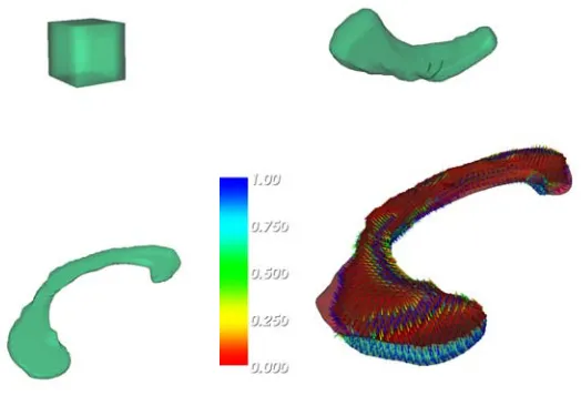
the surface and the final estimated deformation field between the cc of the two patients. For inter-patient studies, such a vector field may be used to obtain a measure of shape and size differences between surfaces of cc’s of two patients and thus proves to be useful.

Fig. 7. Evolution of the surface over the corpus callosum (top row and bottom left) along with the estimated vector field from the first

patient’s corpus callosum (shown in green) towards the second one (shown in red).

Figure 8 shows the T1 MRI volumes of the same brain example from two patients (only one slice from the MRI volume is shown). In this experiment, the “Chan-Vese” flow easily leaks to surrounding regions during the evolutions, therefore does not perform successfully. Instead the “thresholding” flow in Eq. (32) along with the corresponding surface evolution flow Eq. (26) are used with a threshold ofT = 60

whereas the image volumes has the intensity range (0,255). Therefore, with a simple modification to the simplest piecewise constant model and with a quickly obtained prior information from the intensity in the initialized seed surface, we could obtain a reasonable segmentation and registration result as the initial and final contours can be observed in Figure 8.

In the example in Figure 9, two CT image volumes of the same patient taken at different time points are segmented and registered using Eqs. (26)-(30) for delineating the bladder volume at different time periods.

(a) (b)

(c) (d)

Fig. 8. Two sagittal T1 MRI volumes from a patient (a slice shown in a-b) with in-plane resolution 0.44mm and another patient (a slice

shown in c-d) with in-plane resolution 0.97mm: here note the mis-alignment between the corpus callosum of the two patients; after the

non-rigid registration and segmentation has been applied, the resulting corpus callosum surfaces are shown in (b) and (d).

Fig. 9. CT image slices of a patient at different times shown on rows 1 and2. A seed is given in the bladder (left) and the resulting

segmentation and registration on the bladder (middle). The surface shows the deformation of the first surface towards the second (right).

malignant node, exhibit different characteristics. We utilize the piecewise constant model with a non-unit variance termfi = (ˆI(x+u)−mˆf)2

ˆ

σ2 f

χf+(ˆI(x+u_ˆσ2)−mˆb)2 b

Fig. 10. Using a non-unit variance flow, the node on the T2 image (green) is morphed onto the node on the T2* echo image (yellow) on

the right.

B. Experiments in Constrained Problems

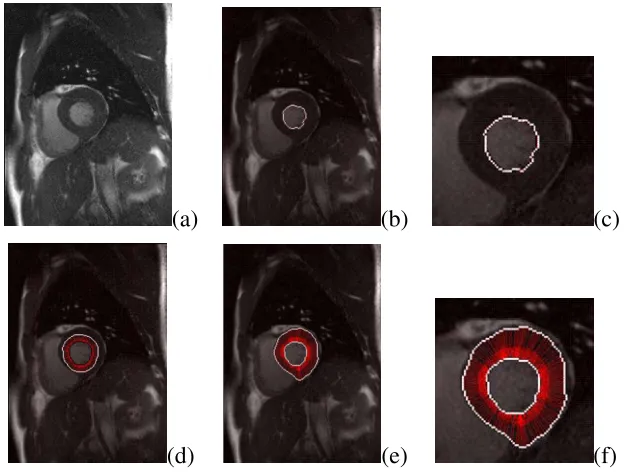
The divergence inequality constraints are applied to segmentation of myocardium in MR images. Figure 11 shows an end-systole phase of the heart beat in (a). Without the divergence constraint terms (39) in our vector field evolution PDE, the image terms can not guarantee a vector field evolution that would keep the solution away from the trivial one, that is a zero vector field as shown in (b) with which the energy of the contour is minimized. Instead, the PDE with divergence constraints leads to the correct solution as shown initially in (d) and result in (e) (zoomed in (f)). In this experiment, the divergence constraint from below (divu ≥c) helps the flow correctly propagate to the solution.

In the next experiment, for the myocardium image at end-diastole in Figure 12(a), the divergence constraint from above (divu ≤ c) steps up to drive the vector field evolution to a better solution in (d) in contrast to the unconstrained PDE result in (c), where both evolutions were initialized with the vector field in (b).

(a) (b) (c)

(d) (e) (f)

Fig. 11. Myocardium image shown at end-systole phase in (a). When there are no constraints on the vector field estimation, the result of

segmentation of the myocardium through the estimated vector field fails because it converges to the trivial solution of zero vector field (b)

(zoomed in (c)). The vector field estimation is successful in case the inequality constraints in (39) are activated initially in (d) and finally in

(e) (zoomed in (f)).

The vector field estimation was successful in case the inequality constraints (54) are activated as shown in (f)-(h).

We show the effect of curl constraint on the vector fields in Figure 14 for the hurricane Katrina sequence (downloaded from National Oceanic and Atmospheric Administration www.noaa.gov). The hurricane is winding outwards from the center in this sequence. The constrained solution is better than the unconstrained solution, as expected. However, the data terms, which we use, do not exactly model this difficult image scenario. If in addition to the constrained PDE terms, one can incorporate good image features that model the image better than piecewise constant mean image, to the data term of the PDEs, the results can be expected to improve.

C. Conclusions

(a) (b) (c) (d)

Fig. 12. Myocardium image shown at end-diastole phase in (a). The initial vector field shown in (b) is evolved without any divergence

inequality constraints in (c), and fails. A better estimation is obtained when the divergence inequality constraints (39) are activated, and

results in a better segmentation of the myocardium through the estimated vector field in (d).

deformations between objects in multiple images. We showed applications in coupled registration and segmentation problems in medical imaging and tracking problems in vision. We believe that our work will stir up new questions and lead to developments in the utilization of inequality constrained variational problems in the computer vision community.

REFERENCES

[1] R. Abraham, J. Marsden, and T. Ratiu. Manifolds, Tensor Analysis and Applications. Springer, 1988.

[2] L. Alvarez, J. Weickert, and J. S´anchez. Reliable estimation of dense optical flow fields with large displacements.International Journal

of Computer Vision, 39(1):41–56, 2000.

[3] Y. Amit. A nonlinear variational problem for image matching. SIAM Journal on Scientific Computing, 15(1):207–224, 1994.

[4] G. Aubert, R. Deriche, and P. Konrprobst. Computing optical flow via variational techniques. SIAM Journal of Applied Mathematics,

60(1):156–182, 1999.

[5] G. A. Bliss. Calculus of Variations. Carus Mathematical Monographs, Chicago, IL, 1925.

[6] T. Chan and L. Vese. An active contour model without edges. InInt. Conf. Scale-Space Theories in Computer Vision, pages 141–151,

1999.

[7] C. Chefd’hotel, G. Hermosillo, and O. Faugeras. A variational approach to multi-modal image matching. InVLSM Workshop-ICCV,

pages 21–28, 2001.

[8] C. Chefd’Hotel, D. Tschumperle, R. Deriche, and O. Faugeras. Regularizing flows for constrained matrix-valued images. Journal of

Mathematical Imaging and Vision, 20:147–162, 2004.

[9] Y. Chen, H. Tagare, S. Thiruvenkadam, F. Huang, D. Wilson, K. Gopinath, R. Briggs, and E. Geiser. Using prior shapes in geometric

(a) (b) (c) (d)

(e) (f) (g) (h)

Fig. 13. Two frames in (a) and (e) from the taxi image sequence (downloaded from KOGS/IAKS Universitat Karlsruhe) demonstrate the

constraint on the norm of the Jacobian of the vector field plus the constraint on the vector field norm itself. (b) and (c) show the resulting

segmentations and vector field estimates when the vector field is evolved without any inequality constraints, hence fails (zoomed section in

(d)). The vector field estimation is successful in case the inequality constraints (54) are activated as depicted in (f) and (g) (zoomed section

in (h)).

[10] A. Cherkaev and E. Cherkaev. Calculus of variations and applications. Lecture Notes, University of Utah, Salt Lake City, UT, 2003.

[11] G. E. Christensen, R. D. Rabbitt, and M. I. Miller. Deformable templates using large deformation kinematics. IEEE Trans. Image

Process., 5(10):1435–1447, 1996.

[12] D. Cremers and S. Soatto. Variational space-time motion segmentation. InProc. Int. Conf. on Computer Vision, pages 886–982, 2003.

[13] M. Desbrun, A. Hirani, and J. Marsden. Discrete exterior calculus for variational problems in computer vision and graphics. InCDC

Conference, 2003.

[14] I. Dydenko, D. Friboulet, and I. Magnin. A variational framework for affine registration and segmentation with shape prior: application

in echocardiographic imaging. InVLSM-ICCV, pages 201–208, 2003.

[15] I. M. Gelfand and S. V. Fomin. Calculus of Variations. Dover Publications, Inc., New York, 1963.

[16] J. Gregory and C. Lin.Constrained Optimization in the Calculus of Variations and Optimal Control Theory. Chapman and Hall, New

York, 1992.

[17] B. K. P. Horn and B. G. Schunck. Determining optical flow. AI, 17:185–203, 1981.

[18] S. Keeling and W. Ring. Medical image registration and interpolation by optical flow with maximal rigidity. Journal of Mathematical

Imaging and Vision, 23(1):47–65, 2005.

[19] D. G. Luenberger. Optimization by Vector Space Methods. John Wiley & Sons, Inc., New York, 1969.

[20] A. Lundervold, T. Taxt, N. Duta, and A. Jain. Model-guided segmentation of corpus callosum in mr images. InProc. IEEE Conf. on

(a) (b) (c)

(d) (e) (f)

Fig. 14. Two frames in (a) and (d) from the hurricane Katrina image sequence demonstrate the constraint on the curl of the vector field.

(b) and (e) show the resulting segmentations (white contour represents the segmentation on the first frame, and black contour on the second

frame, both are shown as superimposed on the second image frame) and vector field estimates when the vector field is evolved without any

inequality constraints, which evolves towards the initial contour without strong features from the image. The vector field estimation is more

likely to be considered as successful in case the inequality constraints of the PDE(44) are activated (c) and (f), although there is no ground

truth knowledge for this example.

[21] J. Modersitzki. Numerical Methods for Image Registration. Oxford University Press, 2004.

[22] D. Mumford and J. Shah. Boundary detection by minimizing functionals. In Proc. IEEE Conf. on Computer Vision and Pattern

Recognition, pages 22–26, San Fransisco, 1985.

[23] S. Osher and J. Sethian. Fronts propagating with curvature dependent speed: Algorithms based on the Hamilton-Jacobi formulation.

J. Computational Physics, 49:12–49, 1988.

[24] N. Paragios and R. Deriche. Geodesic active regions for motion estimation and tracking. InProc. Int. Conf. on Computer Vision, pages

224–240, 1999.

[25] N. Paragios, M. Rousson, and M. Ramesh. Knowledge-based registration and segmentation of the left ventricle: A level set approach.

InIEEE Workshop on App. Comp. Vision, pages 37–42, 2002.

pages 142–165, 2003.

[27] K. Polthier and E. Preuss. Variational approach to vector field decomposition. InEurographics Workshop on Visualization, Springer,

2000.

[28] F. Richard and L. Cohen. A new image registration technique with free boundary constraints: Application to mammography. InProc.

European Conf. Computer Vision, pages 531–545, 2002.

[29] J. Sethian. Level Set Methods and fast marching methods. Cambridge University Press, 1999.

[30] P. Simard and G. Mailloux. A projection operator for the restoration of divergence-free vector fields. IEEE Trans. Pattern Analysis,

and Machine Intelligence, 10(2):248–256, 1988.

[31] Y. Tong, S. Lombeyda, A. Hirani, and M. Desbrun. Discrete multiscale vector field decomposition. InProc. ACM SIGGRAPH, 2003.

[32] G. Unal and G. Slabaugh. Coupled pdes for non-rigid registration and segmentation. InProc. IEEE Conf. on Computer Vision and

Pattern Recognition, volume 1, pages 168–175, 2005.

[33] B. Vemuri and Y. Chen. Geometric Level Set Methods in Imaging, Vision and Graphics, Eds. S.Osher and N.Paragios, chapter Joint

Image Registration and Segmentation, pages 251–269. Springer Verlag, 2003.

[34] F. Wang and B. Vemuri. Simultaneous registration and segmentation of anatomical structures from brain mri. InMICCAI, volume

LNCS 3749, pages 17–25, October 2005.

[35] A. Wong, H. Liu, and P. Shi. Segmentation of myocardium using velocity field constrained front propagation. InIEEE Workshop

Applications of Computer Vision, page 84, 2002.

[36] P. Wyatt and J. Noble. Map mrf joint segmentation & registration. InMICCAI, pages 580–587, 2002.

[37] A. Yezzi, L. Zollei, and T. Kapur. A variational framework for joint segmentation and registration. InCVPR-MMBIA, pages 44–49,

2001.

[38] A. Yezzi, L. Zollei, and T. Kapur. A variational framework for integrating segmentation and registration through active contours.

Medical Image Analysis, 7(2):171–185, 2003.

[39] T. Zhang and D. Freedman. Tracking objects using density matching and shape priors. InProc. Int. Conf. on Computer Vision, pages